High-Capacity Reversible Data Hiding in Encrypted Images Based on Hierarchical Quad-Tree Coding and Multi-MSB Prediction

Abstract

Nowadays, more and more researchers are interested in reversible data hiding in encrypted images (RDHEI), which can be applied in privacy protection and cloud storage. In this paper, a new RDHEI method on the basis of hierarchical quad-tree coding and multi-MSB (most significant bit) prediction is proposed. The content owner performs pixel prediction to obtain a prediction error image and explores the maximum embedding capacity of the prediction error image by hierarchical quad-tree coding before image encryption. According to the marked bits of vacated room capacity, the data hider can embed additional data into the room-vacated image without knowing the content of original image. Through the data hiding key and the encryption key, the legal receiver is able to conduct data extraction and image recovery separately. Experimental results show that the average embedding rates of the proposed method can separately reach 3.504 bpp (bits per pixel), 3.394 bpp, and 2.746 bpp on three well-known databases, BOSSBase, BOWS-2, and UCID, which are higher than some state-of-the-art methods.

1. Introduction

Recently, reversible data hiding (RDH) has gained increasing attention [1,2]. By applying this technique, additional data can be embedded into a multimedia cover [3], while data extraction and original cover recovery can be both realized without loss. Nowadays, with the development of computer technology, digital image becomes the main type of various uploaded data in people’s daily life. Because of its high redundancy, researchers often apply it as the data cover to propose the RDH methods. Most of them in spatial images use three main technologies, i.e., lossless compression [4], difference expansion [5], and histogram shifting [6,7]. These technologies make full use of the redundant information in original images to reversibly embed additional data, but they can only be implemented in the plaintext domain of the image. Once the image is encrypted, lots of redundancy information will be lost. Therefore, the RDH methods based on the above technologies cannot be directly applied to encrypted images.

However, with the increasing popularity of cloud computing and storage applications, people often store or process their privacy data in cloud servers [8,9,10]. Various security issues, such as tampering, forgery, and illegal copying, continuously emerge, which make the privacy protection of digital images attract more and more attention. The RDH methods are suitable for some stringent fields such as medical, military, and legal systems. Therefore, researchers consider combining cryptography with RDH to propose RDHEI methods [11,12,13], which can significantly improve the security of data in the third-party platforms. The RDHEI method is designed for the case that the digital image is encrypted before embedding secret data. The secret data can be embedded without restoring the original image content by the data hider, while the receiver can decrypt the image and conduct data extraction and image recovery without error. Currently, the RDHEI method has been widely applied in the identity authentication, copyright protection, piracy tracking, image management, and so on.

Up to now, many RDHEI methods have been proposed to vacate room for embedding in encrypted image, which is called vacating room after encryption (VRAE) [14,15,16,17]. Zhang presented a VRAE-based RDHEI method in [14]. In this method, a stream cipher is applied to encrypt all the pixels within an uncompressed image. Then this encrypted image is segmented into many blocks, and the pixels in each block are partitioned into two sets. Next, the data hider embeds the additional data through flipping the three least significant bits (LSBs) in one set. After the image decryption, the receiver can use the correlations between adjacent pixels to restore the content of the original image. Based on this method, many researchers presented their improved methods in [15,16,17]. In [15], Yu et al. introduced the flip rate, which further decreased the extraction error-rate and improved the image visual quality after decryption. In [16], Hong et al. adopted the side-match skill in order to better evaluate the block smoothness. In [17], Zhang proposed a separable RDHEI method. In this method, he classified the encrypted images into various groups, and then converted several LSBs of each group into smaller vectors to vacate the embedding room. Finally, the secret data could be extracted from the vacated room before decryption directly.

In the VRAE-based methods, the content owner first performs image encryption, and then the data hider alters some bits of the encrypted image to embed additional data according to certain rules. However, the redundancy of the image is lost after encryption, which results in vacating enough room for embedding very difficult. In order to make full use of image redundancy, some methods about reserving room before encryption (RRBE) [18,19,20,21,22] have been proposed. In [18], Ma et al. proposed the first RRBE-based method. They reserved embedding room in original image by using the histogram shifting technology and encrypted the preprocessed image, then secret data was embedded into certain LSBs in the encrypted region. In [19], Zhang et al. first estimated some pixels through the other adjacent pixels and calculated the estimating errors. Then, the estimating errors and the rest pixels were encrypted by different encryption algorithms, respectively. Finally, they embedded additional data by shifting the estimating error histogram. In [20], Yi and Zhou embedded additional data by applying a binary-block embedding (BBE) scheme. They first divided the MSB planes of original image into lots of blocks, and then vacated room for storing the LSBs by compressing the blocks. Therefore, the additional data could be embedded into lower bit-planes after encryption. In [22], Yi and Zhou also introduced parametric binary tree labeling to propose another RDHEI method, which can exploit the spatial redundancy of encrypted images for data embedding.

In addition, the RRBE-based RDHEI methods can also utilize the redundant information existing in the multi-MSB planes [23,24,25,26,27]. Because it is easier to perform MSB prediction than LSB prediction before image encryption, and there is no need to consider the deterioration of the image quality after encryption, additional data is able to be embedded into the MSB planes. Puteaux et al. gave the first MSB-based method, in which the secret data were embedded by MSB substitution instead of LSB replacement [23]. Since the values of MSBs are modified after embedding, they should be restored without error on the receiver side. Puteaux et al. presented two independent RDHEI methods by separately considering the largest embedding capacity and the complete reversibility. The first method, called high-capacity reversible data hiding approach with correction of prediction errors (CPE-HCRDH), can embed the addition data on the whole MSB plane, though it is not completely reversible. The second one, called high-capacity reversible data hiding approach with embedded prediction errors (EPE-HCRDH), can restore the original image completely without error, but need to mark the position of the prediction error. Subsequently, many researchers proposed several improved RDHEI methods [24,25,26,27] based on [23]. In [24], Puyang et al. extended the EPE-HCRDH method to the MSB plane and the second MSB plane. In [25], Puteaux et al. improved the second method by recursively processing all the bit-planes (from MSB plane to LSB plane). In [26], Chen et al. designed a block-based rearrangement mechanism and extended the run-length code to compress the MSB planes of the original image, which made full use of the redundancy in plaintext domain and effectively freed up the embedding room for secret data. In [27], Yin et al. performed pixel prediction and compressed the differences between the original values and the predicted ones by Huffman coding. They used the stream cipher to execute image encryption, and embedded additional data into the room vacated by the Huffman coding through multiple MSB substitution. Clearly, the amount of data embedded in these two methods is related to the coding schemes closely. Therefore, the researchers try to propose some other good coding schemes in the RDHEI method so as to achieve a high embedded rate of the information.

In this paper, we present a new high-capacity RDHEI method by applying hierarchical quad-tree coding and multi-MSB prediction. Specifically, content owner first performs the pixel prediction to obtain the prediction error. Based on it, the content owner constructs the multi-MSB planes containing concentrated (0)₂ or (1)₂ bit-blocks, where (0)₂ and (1)₂ denote the binary bits. Then, the multi-MSB planes are compressed by hierarchical quad-tree coding so that the embedding room can be reserved before executing the encryption procedure. Next, the content owner encrypts the processed image with the stream cipher. According to the capacity information recorded by the content owner on the LSB plane, additional data can be directly embedded into the encrypted image on the data hider side. The receiver can execute data extraction and image recovery separately with data hiding key and encryption key, respectively. The contributions of this paper include: (1) A hierarchical quad-tree coding scheme with high compression ratio is proposed; (2) data extraction and image recovery can be completed separately; and (3) our method outperforms some of the state-of-the-art methods in embedding rate.

The rest of this paper is organized as follows. Our RDHEI method based on hierarchical quad-tree coding and multi-MSB prediction is described in Section 2. Experimental results, the analysis, and the comparisons with some state-of-the-art methods are given in Section 3. Section 4 gives the conclusions of this paper and the future work.

2. Proposed Method

In this section, we present a new RDHEI method that adopts hierarchical quad-tree coding and multi-MSB prediction. First, the content owner predicts pixels’ value according to their adjacent pixels, calculates the prediction error to construct bit-blocks that have concentrated (0)₂ or (1)₂, and compresses the bit-blocks by using hierarchical quad-tree coding to vacate embedding room. Second, the owner encrypts and scrambles the room-vacated image by the encryption key and the scrambling key, respectively. At the embedding stage, the data hider reversibly scrambles the encrypted image, then directly embeds additional data encrypted by the data hiding key, and finally scrambles the embedded image with the same scrambling key again. The receiver can separately extract the additional data and recover the image by different keys. Our method can achieve high embedding capacity, error-free data extraction, and image recovery. The overview of this proposed method is illustrated in Figure 1, where K_e, K_s, and K_h are the encryption key, the scrambling key, and the data hiding key, respectively.

2.1. Prediction Error Image Generation

For the original gray-level image I_o sized by $M\times N$, content owner first performs the pixel prediction. By applying the median edge detector (MED) predictor [28], predicted pixel values are obtained. As illustrated in Figure 2, the current pixel $p(i,j)$ is predicted through its three adjacent pixels in the previous row and the previous column according to Equation (1). Among it, $1<i\le M$ and $1<j\le N$. The predicted value of $p(i,j)$ is denoted as $\overline{p}(i,j)$.

$$\overline{p}(i,j)=\left\{\begin{array}{ll}\max \{p(i-1,j),p(i,j-1)\},\hfill & \mathrm{if} p(i-1,j-1)\le \min \{p(i-1,j),p(i,j-1)\},\hfill \\ \min \{p(i-1,j),p(i,j-1)\},\hfill & \mathrm{if} p(i-1,j-1)\ge \max \{p(i-1,j),p(i,j-1)\},\hfill \\ p(i-1,j)+p(i,j-1)-p(i-1,j-1),\hfill & \mathrm{otherwise}.\hfill \end{array}\right.$$

(1)

Then, the prediction error of $p(i,j)$, denoted as $p_e(i,j)$, is determined by Equation (2). Next, the decimal $p_e(i,j)$ is converted to binary. The MSBs, denoted as $p_{\mathrm{e}}^0(i,j)$, are used as the sign marker bits since the sign of the prediction error may be positive or negative. Among them, the sign is negative when $p_{\mathrm{e}}^0(i,j)=1$ and positive when $p_{\mathrm{e}}^0(i,j)=0$. The absolute values of the prediction errors are converted into 7-bit sequences according to Equation (3), where $p_{\mathrm{e}}^k(i,j)$ represents the corresponding binary bit. All the sign marker bits $p_{\mathrm{e}}^0(i,j)$ and $p_{\mathrm{e}}^7(i,j)$ form the MSB plane and the LSB plane, respectively. If the absolute value of a prediction error exceeds 127, the corresponding pixel will be recorded as an overflow pixel, and its value will not be altered. Meanwhile, its location (i, j) will be added to auxiliary information, as described in Section 2.3.

$$p_{\mathrm{e}}(i,j)=p(i,j)-\overline{p}(i,j).$$

(2)

$$p_{\mathrm{e}}^k(i,j)=⌊\frac{p_e(i,j) \mathrm{mod} 2^{8-k}}{2^{7-k}}⌋,k=1, 2, \dots , 7.$$

(3)

For example, the current pixel is $p(10, 10)$, and its original value equals 125, seen in Figure 3. According to Equation (1), the predicted value of $p(10, 10)$ is calculated by the values of $p(9, 9)$, $p(9, 10)$, and $p(10, 9)$, i.e., $\overline{p}(10, 10)=130+126-128=128$. Then the prediction error $p_{\mathrm{e}}(10, 10)$ is −3. Obviously, the prediction error is negative, and the binary of its absolute value is 0000011. So we set $p_{\mathrm{e}}^0(10, 10)=1$, $p_{\mathrm{e}}^6(10, 10)=1$, $p_{\mathrm{e}}^7(10, 10)=1$, and the rest bit values are all 0 s, i.e., the binary sequence of $p_{\mathrm{e}}(10, 10)$ is 10000011.

Finally, all the pixels of the original image are scanned by applying the prediction mechanism mentioned above to obtain the prediction error image I_p and the possible invariant pixels. Note that the pixel prediction starts from $p(2, 2)$ row by row and column by column, and the pixels in the first row and the first column serve as the reference pixels.

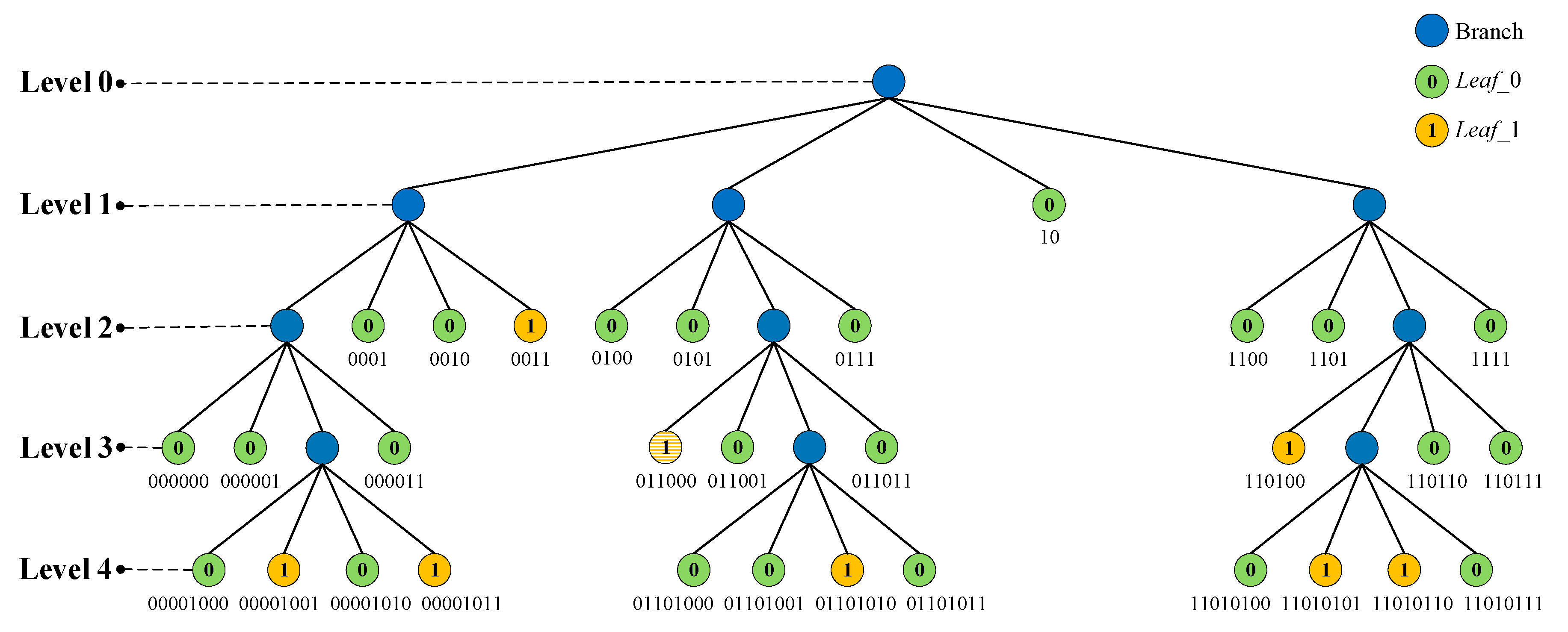
2.2. Hierarchical Quad-Tree Coding

Quad-tree coding is one of the most efficient techniques for compressing highly redundant digital images. Its basic idea is to recursively decompose a $2^n\times 2^n$ (n is a positive integer) pixel array into square regions containing the same pixel value, with the smallest region being a pixel. Owing to the spatial correlation in the prediction error image I_p, the multiple MSB planes of I_p contain a number of bit-blocks that are all 0s or 1s. Thus, we design a hierarchical quad-tree coding to compress the multiple MSB planes of I_p, thereby vacating room for embedding secret data. In our hierarchical quad-tree coding scheme, there are two main steps as follows.

(1) Quad-tree Segmentation

Since I_o has a size of $M\times N$, the size of the eight uncompressed bit-planes of I_p is also $M\times N$. The quad-tree segmentation is implemented sequentially from the MSB plane to the LSB plane of I_p. If $M=N=2^n$, and the bits within the current bit-plane are all the same (all 0s or 1s) before segmentation, and the segmentation will not be implemented, but turned to the next bit-plane until LSB plane. Otherwise, we execute the segmentation process for the current bit-plane as follows. Note that the preprocessed image is denoted as I_g, and the size of I_g denoted by G requires to satisfy Equation (4).

$$G=\left\{\begin{array}{ll}{2}^n\times 2^n,\hfill & \mathrm{if} M=N=2^n,\hfill \\ 2^{⌈{\log }_2\delta ⌉}\times 2^{⌈{\log }_2\delta ⌉},\hfill & \mathrm{if} M=N\ne 2^n \mathrm{or} M\ne N,\delta =\max \{M,N\}.\hfill \end{array}\right.$$

(4)

If $M=N=2^n$, we segment the current bit-plane into four non-overlapping square quadrant blocks. Obviously, the size of each block is $2^{n-1}\times 2^{n-1}$. Then we recursively process each block starting from the top left block, and the recursive order is (I) top left, (II) top right, (III) bottom left, (IV) bottom right, as shown in Figure 4. For each of the four blocks, we first determine whether the bits within the same block are all the same. If so, the segmentation for the current block stops and turns to the next block. Otherwise, the current block is processed recursively. In other words, the current block is segmented into four non-overlapping blocks with the same size of $2^{n-2}\times 2^{n-2}$ if the bits within the current block are not all the same.

If $M=N\ne 2^n$ or $M\ne N$, we denote max (M, N) as δ. Then the size of the current bit-plane is expanded to $2^{⌈{\log }_2\delta ⌉}\times 2^{⌈{\log }_2\delta ⌉}$. The expanded part is added to the right or the bottom of the current bit-plane and filled with 0s. After finishing the expansion, the segmentation is the same as the case of $M=N=2^n$.

After completing the segmentation, we construct a quad-tree corresponding to the current bit-plane. Take the bit-plane of size $16\times 16$ as an example, seen in Figure 5. The corresponding quad-tree is described in Figure 6. The whole bit-plane is taken as the root of the quad-tree and represents level 0. Clearly, when certain parts of the bit-plane require to be further segmented into smaller blocks, the number of levels increases by 1. As shown in Figure 4 and Figure 6, the four nodes from the same tree branch represent the four blocks I, II, III, and IV from left to right. Each of the four nodes is either a leaf node or a branch node. The leaf node represents that the bits within the corresponding block all have the same value (0 or 1), and the branch node indicates that it can be further segmented. In addition, the branch node, which is one level lower than a leaf node, is the parent node of the leaf node.

(2) Hierarchical Quad-tree Coding

Since the quad-tree leaf nodes represent the bit-blocks of a single value, the leaf nodes can be classified into two categories according to the value (0 or 1), denoted by Leaf_0 and Leaf_1, respectively. We first calculate the number of these two categories of leaf nodes in each level of the quad-tree, separately denoted by $Q_0^L$ and $Q_1^L$, where L represents the level of the leaf nodes in the quad-tree. Then, the leaf nodes are encoded hierarchically starting from the root of the quad-tree.

The hierarchical quad-tree coding contains four parts, i.e., the depth coding, the value coding, the number coding, and the path coding of the corresponding leaf nodes, seen in Algorithm 1.

(a)

Depth coding: Here, the depth of leaf nodes is their level denoted by L in quad-tree, which is calculated by Equation (5), where I_b is one bit-plane of I_g, and I_c is the bit-block in I_b corresponding to the specified leaf nodes. L needs to be converted to binary by Equation (3) as the depth code. For the bit-plane of size $2^n\times 2^n$, the depth coding is a fixed-length coding. Let the depth of the root node be 0. Then the maximum depth of the corresponding quad-tree equals n. So at least $⌈{\log }_2(n+1)⌉$ bits are required to record the maximum depth. In other words, the length of depth coding is $⌈{\log }_2(n+1)⌉$.

(b)

Value coding: The value of leaf nodes should be recorded so that the receiver could correctly recover the corresponding leaf nodes. Because there are only two values (0 and 1), it is sufficient for one bit to record the values of leaf nodes.

(c)

Number coding: Since there are at most 4^L nodes in level L, the number of the two categories of leaf nodes in level L, i.e., $Q_0^L$ and $Q_1^L$, is recorded by ${\log }_2(4^L)=2L$ bits.

(d)

Path coding: According to the above quad-tree segmentation process, seen in Figure 4, four quadrant blocks I, II, III, and IV in each round of segmentation correspond to the quadrant codes 00, 01, 10, and 11, respectively. The main idea of path coding is that the corresponding quadrant code is added to the path code each time the segmentation is performed. Obviously, each leaf node requires 2L bits to record its path if the path is encoded separately. In Figure 6, we give an example to show the separate path code of each leaf node, which is composed of their parent nodes’ path codes and their own quadrant codes. However, some leaf nodes usually come from the same parent node and the front $(2L-2)$ bits (i.e., the parent node’s path code) of the path code for these leaf nodes are the same. If these leaf nodes’ path is coded separately, there is a lot of redundancy information. Therefore, we propose a skill to compress the path code in the following. For the leaf nodes in level L, we first encode the path of their parent node, which requires $(2L-2)$ bits. As we know, there are at most three leaf nodes with the same value from a parent node. Thereby, we use 2 bits to record the number of the leaf nodes from the same parent node and these 2 bits are spliced into the end of the parent node’s path code. Finally, we record the quadrant code (00 or 01 or 10 or 11) of each leaf node in order.

$$L={\log }_2\frac{\mathrm{length}({\mathrm{I}}_{\mathrm{b}})}{\mathrm{length}({\mathrm{I}}_{\mathrm{c}})}$$

(5)

Note that if the root node is a leaf node, i.e., the bits within the corresponding bit-plane are all the same, the bit-plane does not need to be segmented. The number coding and the path coding for the root node will not be performed. We only need to record the depth code and the value code. As for the leaf nodes in level 1, their parent node is the root node, and the path coding is not performed for the root node, so the path coding of the leaf nodes in level 1 does not require the compression and just code separately. In other words, the compression of path coding is performed from level 2 to the last level. Because leaf nodes may come from different levels, the number coding and the path coding are both variable-length. The code structure of the leaf nodes in level L is shown in Figure 7.

Algorithm 1 Hierarchical quad-tree coding (HQC) Algorithm

Input: one bit-plane Ib of Ig 1:  /*  t = $⌈{\log }_2(n+1)⌉$                   */ 2:  /*  binary(a, b) is the function that converts a into a b-bit binary sequence */ 3:  /*  B is the path code of nodes                     */ 4:  node ← Ib 5:  function HQC(node) 6:      if the bits in node are not all the same then 7:         [Top_left, Top_right, Bottom_left, Bottom_right] ← SEGMENT(node) 8:         if the bits in Top_left are all the same then result ← CODING(Top_left) 9:         else HQC(Top_left) 10:        end if 11:        if the bits in Top_right are all the same then result ← CODING(Top_right) 12:        else HQC(Top_right) 13:        end if 14:        if the bits in Bottom_left are all the same then result ← CODING(Bottom_left) 15:        else HQC(Bottom_left) 16:        end if 17:        if the bits in Bottom_right are all the same then result ←CODING(Bottom_right) 18:        else HQC(Bottom_right) 19:        end if 20:     else 21:        return result ← CODING(node) 22:     end if 23:  end function 24: 25:  function SEGMENT(node) 26:    node is segmented into four non-overlapping square quadrant blocks Top_left, Top_right, Bottom_left and Bottom_right 27:     result ← [Top_left, Top_right, Bottom_left, Bottom_left] 28:     return result 29:  end function 30: 31:  function CODING(node) 32:     result ← binary(L, t) 33:     if L = 0 then 34:        if value of the node is 0 then result ← result + ‘0’ 35:        else result ← result + ‘1’ 36:        end if 37:     else 38:        if value of the node is 0 then result ← result + ‘0’ + $Q_0^L$ + B 39:        else result ← result + ‘1’ + $Q_1^L$ + B 40:        end if 41:     end if 42:     return result 43:  end function Output: the code of the leaf nodes in level L

After the hierarchical quad-tree coding, we can calculate the code’s length of Leaf_0(s) in level L by Equation (6), denoted by $W_0^L$, where $U_0^L$ indicates the number of the parent nodes of Leaf_0(s) in level L. Then, the embedding capacity denoted by $C_0^L$ and the payload denoted by $D_0^L$ of Leaf_0(s) in level L can be calculated by Equation (7) and (8), respectively. Next, we classify the Leaf_0(s) into available and unavailable categories according to the sign of $D_0^L$. In other words, the Leaf_0s in level L are available if $D_0^L>0$, otherwise they are unavailable. Similarly, we can obtain the available Leaf_1(s) and unavailable Leaf_1(s) through the same classification as Leaf_0(s). For all the available leaf nodes, their codes need to be recorded, but the unavailable leaf nodes do not need to be encoded, and the bits within the corresponding bit-blocks remain unchanged. Thereby, the bit-planes can also be divided into two categories, i.e., the available bit-plane(s) containing the available leaf nodes and the unavailable one(s) without available leaf nodes. Note that the MSB plane is the sign marker plane, and the 0s and the 1s within the MSB plane are relatively evenly distributed. Therefore, the total payload of the MSB plane is usually less than the second MSB plane.

$$W_0^L=\left\{\begin{array}{cc}⌈{\log }_2(n+1)⌉+1,\hfill & \mathrm{if} L=0,\hfill \\ ⌈{\log }_2(n+1)⌉+2L+2\times Q_0^L+1,\hfill & \mathrm{if} L=1,\hfill \\ ⌈{\log }_2(n+1)⌉+2L+2L\times U_0^L+2\times Q_0^L+1,\hfill & \mathrm{if} L\ge 2.\hfill \end{array}\right.$$

(6)

$$C_0^L={(2^{n-L})}^2\times Q_0^L$$

(7)

$$D_0^L=C_0^L-W_0^L$$

(8)

Continue to analyze the example in Figure 6, where the leaf nodes are distributed in levels 1 to 4. First, the length of depth code is calculated, that is $⌈{\log }_2(4+1)⌉=3$. For level 1, the depth code is 001. Because there is only one Leaf_0 in level 1 and its path code is 10, Leaf_1 need not be encoded, and the number code of Leaf_0 is 01. In other words, the code of the leaf node in level 1 is (001 0 01 10). For level 2, the depth code is 010. There are eight Leaf_0s and one Leaf_1, i.e., $Q_0^2$ = 8 = (1000)₂ and $Q_1^2$ = 1 = (0001)₂. The Leaf_0s are encoded first. For the first two Leaf_0s from left to right in level 2, their parent node’s path code is 00 and their quadrant codes are 01 and 10, respectively. So the compressed path code of these two Leaf_0s is (00100110) and the compressed path codes of the rest leaf nodes can be obtained in the same way. Finally, the codes of the Leaf_0s and the Leaf_1 in level 2 are (010 0 1000 00100110 0111000111 1111000111) and (010 1 0001 000111), respectively. Similarly, the codes in level 3 and level 4 can be obtained according to the coding rule mentioned above.

For the example in Figure 6, we can obtain $W_0^1$ = 3 + 2 × 1 + 2 × 1 + 1 = 8, $C_0^1$ = (2^{4 − 1})² × 1 = 64 and $D_0^1$ = 64 − 8 = 56 > 0. So the Leaf_0 in level 1 is available. Similarly, we can also obtain $W_0^2$ = 36, $C_0^2$ = 128, $D_0^2$ = 92 > 0, and $W_1^2$ = 14, $C_1^2$ = 16, $D_1^2$ = 2 > 0. Therefore, the Leaf_0s and the Leaf_1 in level 2 are also the available ones. Obviously, the embedding capacities of each leaf node in the last two levels are only 4 and 1, respectively, which is not enough to carry the corresponding codes. The corresponding payloads are negative, so the leaf nodes in the last two levels are unavailable.

2.3. Vacating Room for Data Embedding

In this subsection, the room for embedding additional data is vacated based on the hierarchical quad-tree coding, seen in Algorithm 2. The quad-tree segmentation and coding are performed on the prediction error image. After executing the hierarchical quad-tree coding for each available bit-plane recursively, there are three parts of information to generate the compressed image containing vacated room:

(1)

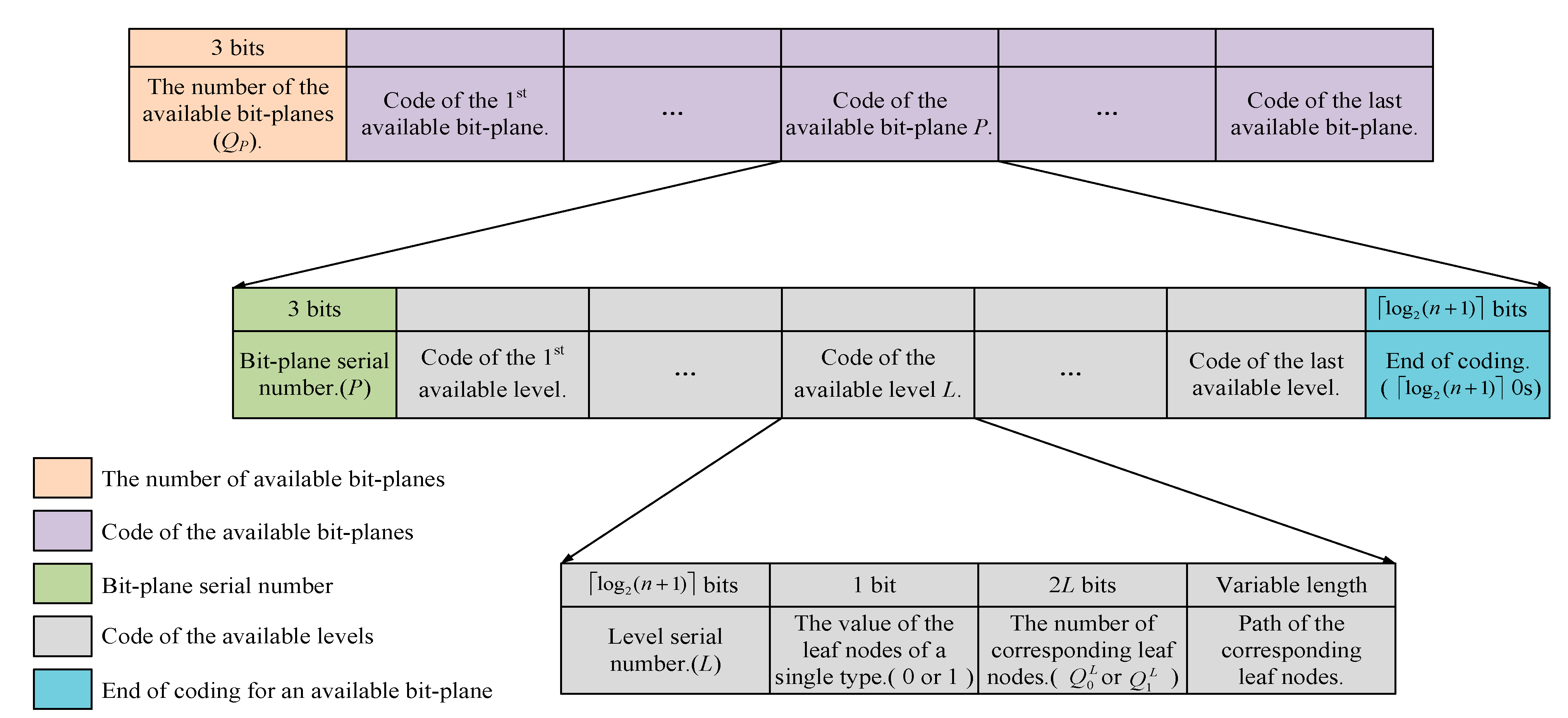
Coding information: For the available bit-planes, we first concatenate all codes of the available leaf nodes in the increasing order of the bit-plane. The code structure is shown in Figure 8. The head of the code structure is the number of available bit-planes, denoted as Q_p, and 3 bits are required to record it. For each available bit-plane, we use 3 bits to record the bit-plane serial number before performing the hierarchical quad-tree coding. Note that the serial number of MSB plane and LSB plane are recorded as 000 and 111, respectively. In addition, $⌈{\log }_2(n+1)⌉$ bits of 0s are required to mark the end of the coding for the current bit-plane.

(2)

Overflow pixels information: We use 2n bits to record the number of overflow pixels which is denoted by Q_x. If Q_x is not equal to 0, the location (i, j) of the overflow pixels also requires to be recorded. Specifically, there are three n-bit parts which need to be recorded, i.e., the row number i, the number of the overflow pixels on i-th row, and the corresponding column number j of each overflow pixel on i-th row. For example, let n be 4 and there are four overflow pixels on the same row. Suppose that their locations are (6,5), (6,7), (6,9), (6,10), respectively. Then the location sequence of these four overflow pixels is (0110 0100 0101 0111 1001 1010).

(3)

Uncompressed bits: The uncompressed bits in each bit-plane are concatenated in the increasing order of the bit-plane serial number and embedded after the information of overflow pixels.

Algorithm 2 Room vacating Algorithm

Input: prediction error image Ip size by M × N, $\delta =\max \{M,N\}$, overflow pixels information 1:   if M = N ≠ 2n or M ≠ N then 2:     Expanding the size to $2^{⌈{\log }_2\delta ⌉}\times 2^{⌈{\log }_2\delta ⌉}$ and the expanded part filled with 0s is added to the right or/and the bottom of the current bit-plane; 3:   end if 4:   Qp ← 0; 5:   code ← [ ]; 6:   uncompressed bits ← [ ]; 7:   for each plane from MSB plane to LSB plane do 8:      Quad-tree segmentation; 9:      Construct a quad-tree corresponds to the current bit-plane; 10:     for each level L from the root to the last level do 11:        Calculate $D_0^L$, $D_1^L$; 12:        if $D_0^L>0$ or $D_1^L>0$ then 13:           Available leaf nodes ← the corresponding leaf nodes; 14:        end if 15:     end for 16:     if the current bit-plane contains available leaf nodes then 17:        Qp ← Qp + 1; 18:        code ← code + (bit-plane serial number + code of the available leaf nodes + end of coding); 19:     end if 20:     uncompressed bits ← uncompressed bits + all bits except the bits in the bit-blocks corresponding to the available leaf nodes; 21:  end for 22:  Record (Qp + code + overflow pixels information + the uncompressed bits) in the multi-MSB planes. 23:  Place the available embedding capacity on the LSB plane. Output: room-vacated image Iv size by M × N

As shown in Figure 9, all of the three parts above are concatenated and recorded in multi-MSB planes. It can be seen that the embeddable bits are located in multi-LSB planes and the net embedding capacity denoted by D is recorded in the last 2n bits of the LSB plane. D can be obtained by Equation (9), where $D_0^{P, L}$ and $D_1^{P, L}$ separately indicate the payload of the available Leaf_0(s) and Leaf_1(s) in level L for the bit-plane P, and D_o indicates the length of the overflow pixels information. Finally, the room-vacated image I_v sized by M × N is generated by Equation (10), where $p_v(i,j)$ is the pixel of I_v and $p_v^k(i,j)$ is the bits of $p_v(i,j)$.

$$D={\displaystyle \sum _{P=0}^7{\displaystyle \sum _{L=0}^n(D_0^{P, L}+D_1^{P, L})}}-D_o-2n$$

(9)

$$p_v(i,j)={\displaystyle \sum _{k=0}^7{p}_v^k(i,j)\times 2^{7-k}}$$

(10)

2.4. Image Encryption

In the phase of image encryption, each bit of the room-vacated image except the embedding capacity bits is encrypted by encryption key K_e, which is first used to generate a pseudo-random matrix q with the size of M × N. Then, the pixel $p_v(i,j)$ and corresponding q(i, j) are converted into binary sequence in accordance with Equation (3), separately denoted by $p_v^k(i,j)$ and $q^k(i,j)$ for k = 0, 1, …, 7. Next, the encryption operation is executed according to Equation (11), where $p_e^k(i,j)$ represents encrypted bits, $\Phi$ represents the set of embedding capacity bits, and $\oplus$ represents the exclusive-or (XOR) operation. The encrypted value p_e(i, j) is obtained by Equation (12) and the encrypted image I_e can be generated.

$$p_e^k(i,j)=\left\{\begin{array}{ll}{p}_v^k(i,j),\hfill & p_v^k(i,j)\in \Phi ,\hfill \\ p_v^k(i,j)\oplus q^k(i,j),\hfill & \mathrm{otherwise}.\hfill \end{array}\right.$$

(11)

$$p_e(i,j)={\displaystyle \sum _{k=0}^7{p}_e^k(i,j)\times 2^{7-k}}.$$

(12)

It should be noted that the embedding capacity bits are not encrypted, so the encrypted image needs to be scrambled for protecting the capacity bits. By adopting the scrambling key K_s, all the pixels in I_e are scrambled. Finally, the scrambled encrypted image ${\mathrm{I}}_e^s$ is obtained.

2.5. Data Embedding

Since multi-LSB planes include the vacated embedding room, data hiding is executed in the vacated multi-LSB planes. The secret data are encrypted by data hider with the data hiding key K_d before embedding, and the location of the vacated room needs to be known first for embedding the data. By adopting the scrambling key K_s, the data hider reversely scrambles the scrambled encrypted image ${\mathrm{I}}_{\mathrm{e}}^{\mathrm{s}}$ to the encrypted image I_e. Then, the vacated room capacity information placed on the LSB plane of I_e can be extracted, and all of the embeddable bits within the multi-LSB planes are obtained. Next, the encrypted secret data is embedded by LSB substitution. After data embedding, the encrypted image containing secret data ${\mathrm{I}}_{\mathrm{e}}^{\mathrm{d}}$ is scrambled again by K_s to obtain the scrambled embedded encrypted image ${\mathrm{I}}_{\mathrm{e}}^{\mathrm{s}, \mathrm{d}}$, which is finally sent to the receiver.

2.6. Data Extraction and Image Recovery

After receiving the scrambled embedded encrypted image ${\mathrm{I}}_{\mathrm{e}}^{\mathrm{s}, \mathrm{d}}$, the legal receiver should reversibly scramble ${\mathrm{I}}_{\mathrm{e}}^{\mathrm{s}, \mathrm{d}}$ with the scrambling key K_s first so that he can extract the secret data from the embedded encrypted image ${\mathrm{I}}_{\mathrm{e}}^{\mathrm{d}}$ with the data hiding key K_d without image decryption. The original image can be restored without loss when the receiver also owns the encryption key K_e. In other words, data extraction and image recovery are separable.

(1) Data Extraction

The embedded data can be extracted from ${\mathrm{I}}_{\mathrm{e}}^{\mathrm{s}, \mathrm{d}}$ directly by the receiver who has keys K_d and K_s. When the legal receiver gets ${\mathrm{I}}_{\mathrm{e}}^{\mathrm{s}, \mathrm{d}}$, he reversely scrambles ${\mathrm{I}}_{\mathrm{e}}^{\mathrm{s}, \mathrm{d}}$ to obtain the embedded encrypted image ${\mathrm{I}}_{\mathrm{e}}^{\mathrm{d}}$ with K_s. Then, the bitstream of embedded secret data is extracted from the multi-LSB planes of ${\mathrm{I}}_{\mathrm{e}}^{\mathrm{d}}$ directly, and the original content of secret data is recovered by using K_d.

(2) Image Recovery

The original image can be recovered without loss by the receiver who has keys K_e and K_s. First, the receiver reversely scrambles ${\mathrm{I}}_{\mathrm{e}}^{\mathrm{s}, \mathrm{d}}$ into the embedded encrypted image ${\mathrm{I}}_{\mathrm{e}}^{\mathrm{d}}$, which can be decrypted into the embedded room-vacated image by using K_e. Because the capacity of the embedding data can be obtained on the LSB plane directly, the secret data is removed from multi-LSB planes and the rest on the multi-MSB planes is the three parts of information corresponding to Section 2.3. The image can be recovered gradually according to the three parts of information.

(a)

Hierarchical Quad-tree Code Recovery

For the coding information in the first part, the number of the available bit-planes Q_p is obtained by converting the front three bits to decimal. Then the available leaf nodes of each available bit-plane can be restored according to the subsequent bits. For the bitstream of each available bit-plane, it starts with the bit-plane serial number recorded by 3 bits, followed by the available leaf nodes code and ends with $⌈{\log }_2(n+1)⌉$ 0s. The bit-blocks corresponding to the available leaf nodes can be restored according to Figure 7, i.e., the recovery of the depth, the value, the number, and the path of the available leaf nodes.

For the code of the available leaf nodes, the front $⌈{\log }_2(n+1)⌉$ binary bits are converted to decimal to obtain the depth, which is the level serial number L of the leaf nodes. Then we scan the subsequent one bit to obtain the values (0 or 1) of the leaf nodes, denoted as β. If L = 0, there is no number code and path code for the current leaf node, otherwise the 2L bits following the value bit are converted to decimals, and the number of the corresponding leaf nodes in level L ($Q_0^L$ or $Q_1^L$) is obtained. Finally, the path codes of the $Q_0^L$ or $Q_1^L$ leaf nodes can be extracted.

For the path code bitstream, if L = 1, the path code of each leaf node is separate and recorded by 2 bits; otherwise, we convert the compressed path code to the separate path code first. If L ≥ 2, the front (2L − 2) bits of the path code are extracted as the path code of the current leaf nodes’ parent node, and the number of the leaf nodes from the same parent node is obtained by the subsequent two bits. The parent node’s path code is then connected with the subsequent 2-bit corresponding quadrant codes as the separate path codes of the leaf nodes from the parent node. After obtaining the separate path codes, the bit-blocks on the bit-plane can be restored without loss. Let the separate path code of each leaf node be $A={\alpha }_1{\alpha }_2{\alpha }_3,\dots ,{\alpha }_2{}_L$. The location of the bit on the upper left of the leaf node’s corresponding bit-block is first determined by Equations (13) and (14), denoted as (I, J). Then the length of the bit-block is calculated by Equation (15).

$$I=1+{\displaystyle \sum _{t=1}^L{2}^n\times 2^{-t}\times {\alpha }_{2t-1}}$$

(13)

$$J=1+{\displaystyle \sum _{t=1}^L{2}^n\times 2^{-t}\times {\alpha }_{2t}}$$

(14)

$${\lambda }^L=2^{n-L}$$

(15)

$$b(i,j)=\beta ,I\le i<I+{\lambda }^L,J\le j<J+{\lambda }^L$$

(16)

Finally, all the bits in the corresponding bit-block are filled with the value of β, shown in Equation (16). Among it, b(i, j) is the bit within the corresponding bit-block. Note that, if the size of the received image M × N does not satisfy M = N = 2ⁿ (that is $M=N\ne 2^n$ or $M\ne N$), the corresponding bit-blocks may not be square, but still satisfies Equation (16). Since the hierarchical quad-tree coding is a lossless compression coding, the compressed blocks can be restored without any loss.

(b)

Overflow Pixels Recovery

For the bitstream of the overflow pixels information in the second part, the front 2n bits are converted to decimals to obtain the number of the overflow pixels Q_x. If Q_x = 0, we turn to the third part of the information. Otherwise, we recover the location of the overflow pixels row by row. For each row containing overflow pixels, the row number i, the number of the overflow pixels on the i-th row, and the column number j of each overflow pixel on the i-th row are all recorded by n bits, respectively. We just extract the n-bits groups in order and convert the combination of the row number and the column number (i, j) to decimals, and then the location of the overflow pixels on the i-th row can be obtained.

(c)

Uncompressed Bits Recovery

For the uncompressed bits in the last part, all of them are filled into the blank bits in order.

After the above steps, we obtain the prediction error image I_p of which the MSB plane is the sign marker plane. Except the reference pixels and overflow pixels (if exist), the pixels in the image are scanned from left to right and top to bottom to restore the predicted pixel values, because the reference pixels and the overflow pixels are preserved after prediction. The predicted value $\overline{p}(i,j)$ of current prediction error $p_e(i,j)$ is obtained by MED predictor, and then the original value $p(i,j)$ can be recovered through $p_e(i,j)$ and $\overline{p}(i,j)$ by Equation (17), where $p_e^0(i,j)$ is the MSB of $p_e(i,j)$. Finally, the original image without error is obtained.

$$p(i,j)=\left\{\begin{array}{ll}\overline{p}(i,j)+p_e(i,j),\hfill & \mathrm{if} p_e^0(i,j)=0,\hfill \\ \overline{p}(i,j)-p_e(i,j)+128,\hfill & \mathrm{if} p_e^0(i,j)=1.\hfill \end{array}\right.$$

(17)

It can be seen that secret data can be extracted reversibly by the receiver who only has the data hiding key K_d and scrambling key K_s, and the lossless original image can be restored only by the encryption key K_e and scrambling key K_s. Thus, this proposed method is separable, reversible, and error-free.

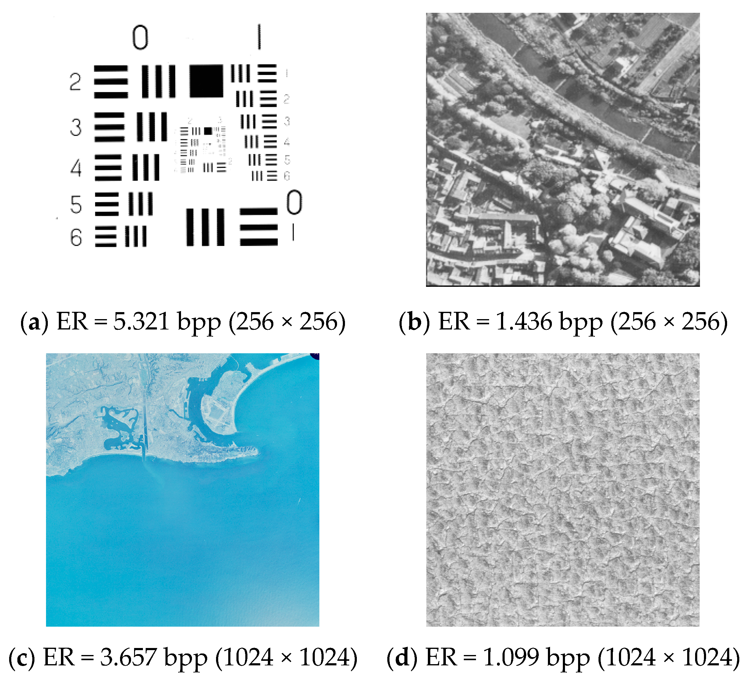
3. Experimental Results and Analysis

In this section, we analyze the security and performance of our method and conduct some experiments to compare our results with some state-of-the-art works based on four usual testing images, Lena, Jetplane, Man, and Baboon, shown in Figure 10. Without loss of generality, we also test in three well-known image databases: BOSSBase [29], BOWS-2 [30], and UCID [31]. There are 10,000 images with sizes of 512 × 512 in BOSSBase [29] and BOWS-2 [30], and 1388 images with sizes of 512 × 384 or 384 × 512 in UCID [31]. These three databases contain a large number of images which are sufficient to verify the performance. Meanwhile, the related researches tend to choose images from these three databases.

3.1. Security Analysis

We first perform pixel prediction and compress the prediction error image based on the hierarchical quad-tree coding to vacate embedding room, and then the room-vacated image is encrypted through a stream cipher. In the following, we will prove our scheme securely from two points of statistical character and probability.

First, the Lena image will be taken as an example, and experimental results of each phase and corresponding histograms obtained by the proposed method are shown in Figure 11 and Figure 12, respectively. Each processing phase of the Lena image with a size of 512 × 512 is shown in Figure 11. Specifically, Figure 11a is the original image, Figure 11b shows the prediction error image based on the MED predictor, Figure 11c is the scrambled encrypted image generated by encryption and scrambling keys K_e and K_s, Figure 11d shows the scrambled embedded encrypted image and its embedding rate (ER) reaches 2.869 bpp, Figure 11e is the image recovered by the scrambling key K_s and the encryption key K_e. From Figure 11c and Figure 11d, it is clear that the scrambled encrypted image and the scrambled embedded encrypted image are highly confused. The correlation among the pixels is already destroyed, and a highly secure ciphertext is generated. In Figure 12, histogram Figure 12a includes meaningful feature information of the original image, histogram Figure 12b indicates that the prediction error image includes many significant edge feature information of the original image, histogram Figure 12c shows the situation of the scrambled encrypted image after stream cipher encryption and scrambling, and histogram Figure 12d shows the situation of the scrambled encrypted image after embedding the secret data. Obviously, it is impossible to obtain any useful statistical feature information from Figure 12c because the pixels are uniformly distributed. Moreover, statistical features of the encrypted image after data embedding and scrambling are still significantly different from the original one, and the distribution of all pixels before and after embedding the secret data is almost similar. Therefore, it is difficult to obtain the content of the original image, which proves that our method is secure enough.

Second, we further discuss the security of our method from the perspective of the probability of restoring the original image without scrambling and encryption keys. With regard to an M × N room-vacated binary image, we encrypt all bits except the embedding capacity bits by a pseudo-random bitstream with the length of $(M\times N\times 8-2\times ⌈{\log }_2\max \{M,N\}⌉ )$, so the number of this pseudo-random sequence is $2^{(M\times N\times 8-2\times ⌈{\log }_2\max \{M,N\}⌉ )}$. In addition, the length of the scrambling key is M × N. So the number of the pseudo-random sequence of the scrambling key is 2^{M × N}. These two numbers are too large. Without knowing the encryption and scrambling keys, the right encryption sequence and scrambling sequence cannot be obtained from so many possibilities. Thus, our method guarantees the confidentiality of original image.

3.2. Performance Analysis

In the prediction phase, we use the MED predictor [28] to obtain predicted pixel values. This predictor can obtain accurate predicted values in most cases, and make the bits with the value of 0 more concentrated on the prediction error planes. A more concentrated plane means shorter codes and less auxiliary information, thereby increasing the ER presented by bpp. The number of the available leaf nodes and their parent nodes can be used to calculate the total capacity of an image. Similarly, the hierarchical quad-tree coding rule and information of the overflow pixels can also be used to calculate the length of the auxiliary information. After obtaining the total capacity and the size of the auxiliary information, the size of the total embedding capacity (EC) and the net payload of an image can be deduced.

For the 512 × 512 Lena image, PSNR of the restored image shown in Figure 11 tends to +∞, and SSIM (structural similarity) equals 1. This means that it is possible to recover the original image without any loss as long as the scrambling and encryption keys are known. Besides, the receiver can restore original data based on the data hiding key because the encrypted secret data can be directly extracted from multi-LSB planes according to the embedding capacity placed on the LSB plane. Figure 13 visually shows the eight quad-tree map planes of the Lena prediction error image. Since the signs of the prediction errors vary greatly on the edge data, the sign marker MSB plane shown in Figure 13a contains a lot of edge information. Clearly, the smooth regions in the multi-MSB planes except the MSB plane correspond to the larger blocks, which means that the predicted multi-MSBs are usually more accurate. While in the rough regions, especially the ones with more edge features, the corresponding blocks are smaller. Since the bits in the multi-LSB planes are uniformly distributed, the smooth regions are few and the corresponding blocks are small. The performance of the quad-tree-based method depends on the number of the large blocks, so the smooth regions in multi-MSB planes are more suitable for quad-tree compression. However, the small rough blocks are not always able to perform compression well or even skip it. Our method exploits the advantages of the quad-tree structure to segment the prediction error planes into blocks of different sizes according to the regional complexity, thereby effectively exploring the characteristics of the prediction error image and improving the performance.

Table 1. Hierarchical quad-tree coding for the Lena image (512 × 512).

Available Plane	${\mathit{Q}}_0^{\mathit{L}}$	${\mathit{U}}_0^{\mathit{L}}$	${\mathit{Q}}_1^{\mathit{L}}$	${\mathit{U}}_1^{\mathit{L}}$	${\mathit{C}}_0^{\mathit{L}}+{\mathit{C}}_1^{\mathit{L}}$ (Bits)	${\mathit{W}}_0^{\mathit{L}}+{\mathit{W}}_1^{\mathit{L}}$ (Bits)	Extra Bits (Bits)	Payload (Bits)
0	188 (L = 7)	114 (L = 7)	45 (L = 7)	32 (L = 7)	3728	2548	7	1173
1	1 (L = 1), 3 (L = 2), 22 (L = 3), 34 (L = 4), 58 (L = 5), 77 (L = 6), 105 (L = 7)	1 (L = 1), 1 (L = 2), 8 (L = 3), 13 (L = 4), 22 (L = 5), 30 (L = 6), 42 (L = 7)	0	0	261,072	2015	7	259,050
2	18 (L = 3), 78 (L = 4), 196 (L = 5), 446 (L = 6), 1028 (L = 7)	9 (L = 3), 37 (L = 4), 86 (L = 5), 201 (L = 6), 440 (L = 7)	0	0	248,768	13,389	7	235,372
3	5 (L = 3), 48 (L = 4), 221 (L = 5), 720 (L = 6), 2335 (L = 7)	5 (L = 3), 30 (L = 4), 104 (L = 5), 351 (L = 6), 1086 (L = 7)	0	0	209,648	27,459	7	182,182
4	2 (L = 4), 39 (L = 5), 571 (L = 6), 3793 (L = 7)	2 (L = 4), 25 (L = 5), 345 (L = 6), 1921 (L = 7)	0	0	109,264	40,174	7	69,083
5	11 (L = 6), 619 (L = 7)	8 (L = 6), 402 (L = 7)	0	0	10,608	7020	7	3581
6	133 (L = 7)	68 (L = 7)	0	0	2128	1237	7	884
7	129 (L = 7)	65 (L = 7)	0	0	2064	1187	7	870
Total	-	-	-	-	847,280	95,029	56	752,195

shows the number of available leaf nodes and their parent nodes distribution, capacity, code length, extra bits, and payload for all available bit-planes of the Lena prediction error image. From Table 1, we can know that the EC of the Lena image is 847,280 bits, the length of hierarchical quad-tree code for all the available bit-planes is 95,029 bits, the length of the extra bits for each available bit-plane (that is the bit-plane serial number and the end of the code for the bit-plane) is 7 bits, and the total is 56 bits. Obviously, the EC minus the sum of the total code length and the amount of extra bits for the available bit-planes is 752,195 bits, which can also be obtained from the payload of each available plane in the last column of Table 1. Additionally, 3 bits, 18 bits, and 18 bits are required to store the number of the available bit-planes, the overflow pixel information, and the length of the total EC, respectively. Therefore, the total EC and the final payload are 752,156 bits and 2.869 bpp, as seen in

Table 2. Total embedding capacity and auxiliary information for the Lena image.

Qp Length (Bits)	Qx	Do (Bits)	EC Length (Bits)	Total EC (Bits)	Net Payload (Bpp)
3	0	18	18	752,156	2.869

. Furthermore, we show the experimental results of all four test images in

Table 3. Experimental results on different testing images.

Testing Images	Capacity (Bits)	Code Length (Bits)	Total Extra Bits (Bits)	Total EC (Bits)	Net Payload (Bpp)
Lena	847,280	95,029	95	752,156	2.869
Jetplane	950,592	99,319	108	851,165	3.247
Man	764,080	117,486	115	646,479	2.466
Baboon	410,736	77,433	130	333,173	1.271

. The net payloads of Lena, Jetplane, Man, and Baboon based on our method reach 2.869 bpp, 3.247 bpp, 2.466 bpp, and 1.271 bpp, respectively.

Furthermore, we apply our method to conduct some experiments in three databases BOSSBase [29], BOWS-2 [30], and UCID [31]. Because the bits with the value 0 on the prediction error planes are more concentrated for the relatively smooth images, the total EC is larger, and the length of hierarchical quad-tree code is shorter. As a result, more secret data can be embedded, which means a larger net payload. On the contrary, the net payload of the rough images is smaller because of the smaller total EC and larger auxiliary information. In

Table 4. Experimental results on three image databases.

Databases		BOSSbase [29]	BOWS-2 [30]	UCID [31]
Best case	ER (bpp)	7.824	7.145	5.335
	PSNR	+∞	+∞	+∞
	SSIM	1	1	1
Worst case	ER (bpp)	0.476	0.418	0.192
	PSNR	+∞	+∞	+∞
	SSIM	1	1	1
Average	ER (bpp)	3.504	3.394	2.746
	PSNR	+∞	+∞	+∞
	SSIM	1	1	1

, we list the best case, the worst case, and the average value of three indicators ER, PSNR, and SSIM for the three databases. For database BOSSBase, ER reaches from 7.824 bpp to 0.476 bpp with the average value 3.504 bpp. For database BOWS-2, ER reaches from 7.145 bpp to 0.418 bpp with the average value 3.394 bpp. For database UCID, ER reaches from 5.335 bpp to 0.192 bpp with the average value 2.746 bpp. Meanwhile, all of the images can be restored without loss, i.e., PSNR → +∞ and SSIM = 1. In additional, the SIPI [32] database contains 73 images of a size of 256 × 256 and 53 images of a size of 1024 × 1024. In order to evaluate the performance for images with other sizes, we also apply our method to conduct experiments on these two types of images from the SIPI database. For the 256 × 256 images, ER reaches from 5.321 bpp to 1.436 bpp with the average value 2.711 bpp. For the 1024 × 1024 images, ER reaches from 3.657 bpp to 1.099 bpp with the average value 2.251 bpp. The corresponding results and some images are given in

Table 5. Experimental results on 256 × 256 and 1024 × 1024 images from the SIPI [32] database.

Image Size		256 × 256	1024 × 1024
Best case	ER (bpp)	5.321	3.657
	PSNR	+∞	+∞
	SSIM	1	1
Worst case	ER (bpp)	1.436	1.099
	PSNR	+∞	+∞
	SSIM	1	1
Average	ER (bpp)	2.711	2.251
	PSNR	+∞	+∞
	SSIM	1	1

and Figure 14. These results indicate the excellent performance of our method in the protection of sensitive data.

3.3. Comparison with Some State-of-the-Art Methods

In this subsection, we compare our method with six state-of-the-art ones [22,23,24,25,26,27]. Figure 15 shows the comparison results of ER on four testing images including Lena, Jetplane, Man, and Baboon. Among them, the Baboon image gains the lowest ER because it is rough and there is too much auxiliary information recorded. In our method, the largest embedding room is explored in the prediction error image by hierarchical quad-tree coding for improving the ER of rough images. Clearly, our method outperforms the six previous methods as the aspect of ER on the four testing images even for the rough image Baboon with high auxiliary information, as seen in Figure 15.

In order to further show the advantage of our method, we conduct some experiments in three databases [29,30,31]. The average ERs of our method in BOSSBase, BOWS-2, and UCID reach 3.504 bpp, 3.394 bpp, and 2.746 bpp, respectively. In Figure 16, we list some detailed comparison results for each database by applying our method and the state-of-the-art ones.

Table 6. Net payload comparison on different image databases (bpp).

Image Databases	Net Payload of Different Methods
	[23]	[24]	[25]	[22]	[26]	[27]	Proposed Method
BOSSbase [29]	0.966	1.447	1.999	1.957	2.323	3.361	3.504
BOWS-2 [30]	0.968	1.346	1.836	1.881	2.245	3.246	3.394
UCID [31]	0.893	1.179	1.035	1.586	1.877	2.688	2.746

shows the detailed information of net payload in different image databases applying different methods. Clearly, our method can increase the average ER of three databases. These results show that our method outperforms some previously known ones from the average ER.

4. Conclusions

In this paper, we apply hierarchical quad-tree coding and multi-MSB prediction to present a new RDHEI method with high embedding rate. Content owner calculates the prediction error to make the multi-MSB planes more concentrated and compresses redundant information by using the hierarchical quad-tree coding to vacate larger embedding room. The data hider can embed additional data without knowing the content of the original image. Data extraction and image recovery can be performed separately on the receiver side. Our method applies hierarchical quad-tree coding, which makes the blocks corresponding to the available leaf nodes compressed adequately and vacated more room for embedding. Meanwhile, vacating room before image encryption can make the most of the redundancy in the prediction error image. Specifically, the total embedding capacity can be deduced by the number of overflow pixels, the available leaf nodes and their parent nodes based on the quad-tree segmentation on each available prediction error plane. Experimental results show that the proposed method has excellent performance in privacy protection and higher embedding rate compared with some state-of-the-art methods.

However, as can be seen from the experimental results of rough images, the embedding rate is still low due to the large amount of auxiliary information and small redundancy. Therefore, we are interested in improving prediction performance or other bit-plane rearrangement mechanism in the future work. Because a more accurate prediction results in the smoother prediction error planes, which can increase the embedding capacity. In addition, the more accurate prediction algorithm or a better bit-plane rearrangement mechanism is used, the fewer overflow pixels will be, thereby reducing the length of auxiliary information and improving the performance of the method.

References

1. Shi, Y.; Li, X.; Zhang, X.; Wu, H.; Ma, B. Reversible data hiding: Advances in the past two decades. IEEE Access 2016, 4, 3210–3237. [Google Scholar] [CrossRef]
2. Chang, C.-C. Adversarial learning for invertible steganography. IEEE Access 2020, 8, 198425–198435. [Google Scholar] [CrossRef]
3. Chang, Y.; Liu, C.-C.; Nguyen, T.S. A Novel Turtle Shell Based Scheme for Data Hiding. In Proceedings of the 2014 International Conference on Intelligent Information Hiding and Multimedia Signal Processing, Kitakyushu, Japan, 27–29 August 2014; pp. 89–93. [Google Scholar]
4. Celik, G.; Sharma, M.U.; Tekalp, A.M.; Saber, E. Lossless generalized-LSB data embedding. IEEE Trans. Image Process. 2005, 14, 253–266. [Google Scholar] [CrossRef]
5. Tian, J. Reversible data embedding using a difference expansion. IEEE Trans. Circuits Syst. Video Technol. 2003, 13, 890–896. [Google Scholar] [CrossRef] [Green Version]
6. Li, X.; Li, B.; Yang, B.; Zeng, T. General framework to histogram-shifting-based reversible data hiding. IEEE Trans. Image Process. 2013, 22, 2181–2191. [Google Scholar] [CrossRef]
7. Wang, J.; Ni, J.; Zhang, X.; Shi, Y. Rate and distortion optimization for reversible data hiding using multiple histogram shifting. IEEE Trans. Cybern. 2017, 47, 315–326. [Google Scholar] [CrossRef] [PubMed]
8. Chang, C.-C.; Li, C.-T.; Shi, Y. Privacy-aware reversible watermarking in cloud computing environments. IEEE Access 2018, 6, 70720–70733. [Google Scholar] [CrossRef]
9. Chang, C.-C.; Li, C.-T.; Chen, K. Privacy-Preserving Reversible Information Hiding Based on Arithmetic of Quadratic Residues. IEEE Access 2019, 7, 54117–54132. [Google Scholar] [CrossRef]
10. Chang, C.-C.; Li, C.-T. Algebraic secret sharing using privacy homomorphisms for IoT-based healthcare systems. Math. Biosci. Eng. 2019, 16, 3367–3381. [Google Scholar] [CrossRef]
11. Puech, W.; Chaumont, M.; Strauss, O. A reversible data hiding method for encrypted images. In Proceedings of the Security, Forensics, Steganography, and Watermarking of Multimedia Contents X, International Society for Optics and Photonics, San Jose, CA, USA, 18 March 2008; Volume 6819, pp. 534–542. [Google Scholar]
12. Yi, S.; Zhou, Y.; Hua, Z. Reversible data hiding in encrypted images using adaptive block-level prediction-error expansion. Signal Process. Image Commun. 2018, 64, 78–88. [Google Scholar] [CrossRef]
13. Huang, D.; Wang, J. High-capacity reversible data hiding in encrypted image based on specific encryption process. Signal Process. Image Commun. 2020, 80, 115632. [Google Scholar] [CrossRef]
14. Zhang, X. Reversible data hiding in encrypted image. IEEE Signal Process. Lett. 2011, 18, 255–258. [Google Scholar] [CrossRef]
15. Yu, J.; Zhu, G.; Li, X.; Yang, J. An improved algorithm for reversible data hiding in encrypted image. In Proceedings of the International Workshop on Digital Forensics and Watermarking, Shanghai, China, 31 October–3 November 2012; Volume 7809, pp. 384–394. [Google Scholar]
16. Hong, W.; Chen, T.; Wu, H. An improved reversible data hiding in encrypted images using side match. IEEE Signal Process. Lett. 2012, 19, 199–202. [Google Scholar] [CrossRef]
17. Zhang, X. Separable reversible data hiding in encrypted image. IEEE Trans. Inf. Forensics Secur. 2012, 7, 826–832. [Google Scholar] [CrossRef]
18. Ma, K.; Zhang, W.; Zhao, X.; Yu, N.; Li, F. Reversible data hiding in encrypted images by reserving room before encryption. IEEE Trans. Inf. Forensics Secur. 2013, 8, 553–562. [Google Scholar] [CrossRef]
19. Zhang, W.; Ma, K.; Yu, N. Reversibility improved data hiding in encrypted images. Signal Process. 2014, 94, 118–127. [Google Scholar] [CrossRef]
20. Yi, S.; Zhou, Y. Binary-block embedding for reversible data hiding in encrypted images. Signal Process. 2017, 133, 40–51. [Google Scholar] [CrossRef]
21. Shiu, P.; Tai, W.; Jan, J.; Chang, C.-C.; Lin, C. An Interpolative AMBTC-based high-payload RDH scheme for encrypted images. Signal Process. Image Commun. 2019, 74, 64–77. [Google Scholar] [CrossRef]
22. Yi, S.; Zhou, Y. Separable and reversible data hiding in encrypted images using parametric binary tree labeling. IEEE Trans. Multimed. 2019, 21, 51–64. [Google Scholar] [CrossRef]
23. Puteaux, P.; Puech, W. An efficient MSB prediction-based method for high-capacity reversible data hiding in encrypted images. IEEE Trans. Inf. Forensics Secur. 2018, 13, 1670–1681. [Google Scholar] [CrossRef] [Green Version]
24. Puyang, Y.; Yin, Z.; Qian, Z. Reversible data hiding in encrypted images with two-MSB prediction. In Proceedings of the 2018 IEEE International Workshop on Information Forensics and Security (WIFS), Hong Kong, China, 11–13 December 2018. [Google Scholar]
25. Puteaux, P.; Puech, W. EPE-based huge-capacity reversible data hiding in encrypted images. In Proceedings of the 2018 IEEE International Workshop on Information Forensics and Security (WIFS), Hong Kong, China, 11–13 December 2018. [Google Scholar]
26. Chen, K.; Chang, C.-C. High-capacity reversible data hiding in encrypted images based on extended run-length coding and block-based MSB plane rearrangement. J. Vis. Commun. Image Represent. 2019, 58, 334–344. [Google Scholar] [CrossRef]
27. Yin, Z.; Xiang, Y.; Zhang, X. Reversible data hiding in encrypted images based on multi-MSB prediction and Huffman coding. IEEE Trans. Multimed. 2020, 22, 874–884. [Google Scholar] [CrossRef]
28. Weinberger, G.; Seroussi, M.J.; Sapiro, G. The LOCO-I lossless image compression algorithm: Principles and standardization into JPEG-LS. IEEE Trans. Image Process. 2000, 9, 1309–1324. [Google Scholar] [CrossRef] [PubMed] [Green Version]
29. Bas, P.; Filler, T.; Pevny, T. Break our steganographic system: The ins and outs of organizing BOSS. In Proceedings of the 13th International Conference on Information Hiding, Prague, Czech Republic, 18–20 May 2011; pp. 59–70. [Google Scholar]
30. Bas, P.; Furon, T. Image Database of BOWS-2. Available online: http://bows2.ec-lille.fr/ (accessed on 17 July 2007).
31. Schaefer, G.; Stich, M. UCID—An uncompressed color image database. In Proceedings of the SPIE in Storage and Retrieval Methods and Applications for Multimedia, San Jose, CA, USA, 18–22 January 2004; Volume 5307, pp. 472–480. [Google Scholar]
32. Weber, A.G. The USC-SIPI image database version 5. USC-SIPI Rep. 1997, 315, 1. [Google Scholar]
Figure 1. The overview of the proposed method.
Electronics 10 00664 g001
Figure 2. The pixel location for the median edge detector (MED) predictor.
Electronics 10 00664 g002
Figure 3. An example of calculating a prediction error. (a) The original values of the current pixel p ( 10 ,   10 ) and its three adjacent pixels p ( 9 ,   9 ) , p ( 9 ,   10 ) , and p ( 10 ,   9 ) are 125, 128, 130, and 126, respectively; (b) the predicted value of p ( 10 ,   10 ) is calculated with MED predictor, i.e., p ¯ ( 10 ,   10 ) = 130 + 126 128 = 128 ; (c) The prediction error of p ( 10 ,   10 ) is calculated as p e ( 10 ,   10 ) = p ( 10 ,   10 ) p ¯ ( 10 ,   10 ) = 125 128 = 3 .
Electronics 10 00664 g003
Figure 4. Quad-tree segmentation for bit-block with size of 2 n × 2 n .
Electronics 10 00664 g004
Figure 5. An example of quad-tree segmentation for one bit-plane of prediction error image (n = 4). The bits are not all the same on the original bit-plane, so the original bit-plane is segmented into four non-overlapping square blocks. In the first, second, and fourth blocks, the bits are not all the same, and segmentation is performed recursively until the bits in a block are all the same. The third block need not to be further segmented because the bits within it are all the same.
Electronics 10 00664 g005
Figure 6. The quad-tree and the separate path coding of the leaf nodes corresponding to Figure 5.
Electronics 10 00664 g006
Figure 7. The code structure of the available leaf nodes in level L.
Electronics 10 00664 g007
Figure 8. The hierarchical quad-tree code structure for the processed image.
Electronics 10 00664 g008
Figure 9. Room-vacated image planes.
Electronics 10 00664 g009
Figure 10. Four testing images.
Electronics 10 00664 g010
Figure 11. The experimental results on Lena image: (a) Original image; (b) prediction error image; (c) scrambled encrypted image; (d) scrambled embedded encrypted image with net payload ER = 2.869 bpp; (e) restored image, peak signal-to-noise ratio (PSNR) = +∞.
Electronics 10 00664 g011
Figure 12. Frequency statistics of Lena image in four phases: (a) The original image histogram; (b) the prediction error image histogram; (c) the scrambled encrypted image histogram; (d) the scrambled embedded encrypted image histogram.
Electronics 10 00664 g012
Figure 13. Quad-tree map planes of Lena prediction error image.
Electronics 10 00664 g013aElectronics 10 00664 g013b
Figure 14. Corresponding images from the SIPI [32] database. http://sipi.usc.edu/database/ (access on 1 January 2021).
Electronics 10 00664 g014
Figure 15. Comparisons between the proposed method and the current state-of-the-art methods [22,23,24,25,26,27] on four testing images.
Electronics 10 00664 g015
Figure 16. Performance comparisons between our method and [22,23,24,25,26,27] in different image databases BOSSbase [29], BOWS-2 [30], and UCID [31].
Electronics 10 00664 g016