Article

Per-Core Power Modeling for Heterogenous SoCs

1
School of Electrical Engineering and Computer Science, Washington State University, Pullman, WA 99164, USA
2
Department of Electrical and Computer Engineering, University of Wisconsin–Madison, Madison, WI 53706, USA
3
School of Electrical, Computer and Energy Engineering, Arizona State University, Tempe, AZ 85287, USA
4
Futerwei Technologies, Santa Clara, CA 95050, USA
*
Authors to whom correspondence should be addressed.
Electronics 2021, 10(19), 2428; https://doi.org/10.3390/electronics10192428
Submission received: 23 August 2021 / Revised: 29 September 2021 / Accepted: 1 October 2021 / Published: 7 October 2021
(This article belongs to the Section Microelectronics)

Abstract

:
State-of-the-art mobile platforms, such as smartphones and tablets, are powered by heterogeneous system-on-chips (SoCs). These SoCs are composed of many processing elements, including multiple CPU core clusters (e.g., big.LITTLE cores), graphics processing units (GPUs), memory controllers and other on-chip resources. On the one hand, mobile platforms need to provide a swift response time for interactive apps and high throughput for graphics-oriented workloads; on the other hand, the power consumption must be under tight control to prevent high skin temperatures and energy consumption. Therefore, commercial systems feature a range of mechanisms for dynamic power and temperature control. However, these techniques rely on simple indicators, such as core utilization and total power consumption. System architects are typically limited to the total power consumption, since multiple resources share the same power rail. More importantly, most of the power rails are not exposed to the input/output pins. To address this challenge, this paper presents a thorough methodology to model the power consumption of major resources in heterogeneous SoCs. The proposed models utilize a wide range of performance counters to capture the workload dynamics accurately. Experimental validation on a Nexus 6P phone, powered by an octa-core Snapdragon 810 SoC, showed that the proposed models can estimate the power consumption within a 10% error margin.

1. Introduction

Mobile platforms have become ubiquitous due to their crucial role in enabling everyday tasks, such as messaging, calling, gaming, navigation, and web browsing [1]. This success is primarily due to heterogeneous SoCs, which provide competitive performance in a mobile form factor [2,3]. Since the mobile form factor rules out active cooling and large batteries, heterogeneous SoCs have low power consumption (<10 W) and high energy efficiency [4,5,6]. These requirements are satisfied by integrating general-purpose CPUs, many specialized processing elements (PEs), and a high-bandwidth interconnection network on a single die. For example, graphics processing units (GPUs), display processing engines, and audio processors, have become standard components of state-of-the-art SoCs [2,7,8,9]. Any specialized function, such as display rendering, is performed in the corresponding PE, achieving higher performance and lower power consumption than a general-purpose core. As a result, both the overall system energy efficiency and the power consumption are improved significantly compared to a system that consists of only CPU cores.
Power consumption has been one of the primary design considerations for more than a decade [10,11,12]. Hence, energy-efficient techniques have been widely studied to harness the processing power within available power and thermal budgets [13,14,15,16,17,18]. With the proliferation of mobile devices, the criticality of energy efficiency is multiplied. On the one hand, increasing the computational power, and sensing, storage, and communication capabilities, opens up a wide range of power-hungry application domains; on the other hand, battery life rises as one of the major concerns to end-users [19,20]. As a result, power management techniques crafted specifically for smart mobile devices become necessary. Although state-of-the-art SoCs have tens of PEs, only a few PEs need to be active in typical use cases [7,21]. For instance, one CPU core and wireless modem are enough during texting on a smartphone. Consequently, optimal energy efficiency in smart mobile devices can be achieved only if the platform components are considered as a whole rather than treating individual components in isolation [22]. Therefore, the power consumption of major PEs should be modeled accurately. Then, dynamic thermal and power management (DTPM) algorithms can utilize these models to control each PE more effectively [11,23,24,25,26,27,28].
The most power-hungry components of state-of-the-art heterogeneous SoCs change as a function of the workload [1,29]. For example, big.LITTLE CPU cluster power consumption dominates when running CPU-intensive applications, while GPU power consumption becomes dominant during the playing of graphics-intensive games. In general, the dominant sources of power consumption are the display, CPU clusters, and GPU. Therefore, SoC manufacturers implement knobs to control the power states of these devices. For example, the Nexus 6P phone with a Snapdragon 810 SoC [30], used in the experimental evaluations, allows for control of the bandwidths of the CPU and GPU memory controllers using OS drivers. Before making control decisions, the controller has to evaluate the effect of the control decisions on the system. State-of-the-art power management techniques can model and analyze CPU and GPU power [27,31,32,33,34]. In order to analyze the effect of changing various control knobs, it is necessary to build the power models for the respective components. Therefore, this paper models the power consumption of the following major components of a mobile SoC: (1) the AMOLED display, (2) the big CPU cluster with four ARM A57 cores, (3) the little CPU cluster with four ARM A53 cores, (4) the Adreno 430 GPU, (5) the CPU memory controller, and (6) the GPU memory controller. The proposed models are straightforward to implement on a smartphone because they involve linear equations that can be computed in constant time. The input features required for the models are available in the Linux kernel through the performance monitoring unit. These counters are read by the governors at runtime to estimate the power consumption and make power management decisions. The models are validated by performing extensive experiments on the Nexus 6P phone.
The novel contributions of this paper are:
  • different components which contribute to the total power consumed by the Nexus 6P phone are identified;
  • each component of the power is accurately modeled through linear regression; and,
  • obtained models are evaluated extensively to show the efficiency of the proposed power modeling technique for the Nexus 6P phone.
The rest of this paper is organized as follows: Section 2 describes the proposed modeling methodology and the tools used in this work, Section 3 presents the main results, and Section 4 concludes the paper.

2. Materials and Methods

2.1. Overview of the Overall Modeling Methodology

The per-core power consumption modeling methodology adopted in this work is shown in Figure 1. Since commercial phones do not provide access to individual power rails, only the total power drawn by the phone can be measured. Therefore, a data acquisition system (DAQ) was used to measure the total power, following the method described in Section 2.2. Then, the power consumption of the individual components were modeled, and subtracted from the total power one-by-one, as outlined in Figure 1.
The modeling process started with the display power consumption since it was easier to isolate from the rest of the components (Section 3.1). After the model for the display power was computed, it was subtracted from the total power consumption to obtain the power consumption of the SoC and other parts in the system. The SoC power consumption consists of the leakage and dynamic components of the PEs. In the power modeling flow, the leakage power consumption was first modeled by running a light workload. The dynamic activity was kept fixed and the experiments were repeated at different temperatures. In this way, the model captures the dependence of leakage power on the temperature. Then, the leakage power was subtracted from the SoC power consumption to find the dynamic power consumption. Next, the frequency of the PEs was swept to collect the power consumption, temperature, and a variety of hardware performance counters, at each desired frequency. Finally, the dynamic power consumption of each PE was modeled as a function of the frequency and performance counters. These steps are detailed for the big core cluster, little core cluster, GPU, CPU memory controller, and GPU memory controller in Section 3.2 through Section 3.6. The following subsection describes the tools used in all the power modeling steps.

2.2. Tools Used in this Work

Nexus 6P phone (Huawei, Shenzhen, China): In this work, the power consumption of the Snapdragon 810 SoC [30] was modeled. The SoC contains four A57 big cores and four A53 little cores. The chipset also has an Adreno 430 GPU driving a 1440 × 2560 AMOLED display. The Nexus 6P runs on an Android-7.1. Nougat with a Linux 3.10 kernel. The Nexus 6P phone was chosen since it uses the Snapdragon 810 processor, and many new smartphones use the same family processor with similar heterogeneity. Furthermore, the software source code for the Nexus 6P is freely available, which makes it straightforward to add instrumentation for performance counters.
To model the system’s power consumption, the total power consumption of the device needs to be measured. To enable power consumption measurement, firstly, the internal battery was disconnected without removing it from the phone. Then, an external power supply was connected to the power supply terminal of the phone using a connector, similar to the one used by the disconnected battery, as shown in Figure 2 and described next.
NI PXIe-1071 data acquisition system: The National Instruments PXIe-1071 data acquisition (DAQ) system was used to perform all the power consumption measurements. A Labview interface was used to control the measurement of the power consumption from the host system. The phone was connected to a power supply through a 0.01 Ω shunt resistor. The DAQ measures the voltage across the shunt resistor at a sampling rate of 1 KHz. The measured voltage was used to calculate the current drawn by the phone. Then, the current was multiplied by the supply voltage at the phone’s terminal to compute the power consumption.
Instrumentation of performance data collection: The on-demand governor in the kernel was instrumented to profile features such as the number of instructions, CPU utilization, GPU utilization, the number of memory bytes used, the number of memory accesses, and the number of L2 cache misses. The OS called the instrumented code periodically to read these counters. The period was set to 50 ms using the sysfs interface to achieve high granularity without any noticeable overhead. After instrumenting the kernel, the kernel was re-built and flashed onto the phone. The Android system was not rebuilt since the files in the Android system were not changed. Additionally, the SimplePerf [35] tool was used to obtain CPU hardware performance counter information as follows:
$./simpleperf stat -a --csv -e instructions:u,cpu-cycles:u,cache-references:u,cache-misses:u,branch-misses:u,raw-mem-access:u --interval 50 -o $filename (Command 1)
The first two arguments in command 1 ensure that it continuously gathers the performance statistics for all CPUs. The --csv argument lets the tool know that the gathered data is written into a readable csv file format. Then, the -e argument specifies the counters that are to be profiled while the application is running. The --interval argument specifies the interval at which the performance counters are collected.

2.3. Pre-Processing the Raw Power Consumption Measurements

Data collected from the NI-DAQ was subjected to several sources of noise. One of the major contributors to noise is the main power line. The power line contributes noise at 60 Hz and its harmonics, since the electrical power supply frequency in the United States is 60 Hz. In order to mitigate this noise, the power line noise was filtered through a series of five notch filters with center frequencies at 60 Hz, 120 Hz, 180 Hz, 240 Hz, and 300 Hz. Each of these filters has a bandwidth of 4 Hz centered around the respective center frequency. A bandwidth of 4 Hz was chosen since it is low enough to exclude some frequencies without excluding other useful frequencies. Then, the low-frequency noise was removed using a low pass filter with a cutoff frequency of 400 Hz. The cutoff frequency was 400 Hz as the frequency of power consumption changes was expected to be lower than 400 Hz. This is for the following reasons:
Frequency and voltage management governors in smartphones, such as on-demand and interactive, make frequency and voltage changes every 50 ms. This means that the change in power consumption due to voltage and frequency levels occurs at about 20 Hz.
The frequency response in Figure 3a shows that the magnitude of higher frequencies is much lower than the smaller frequencies. In fact, the box in Figure 3a shows that the frequency response was concentrated between −50 Hz and 50 Hz.
Figure 3 shows a sample power consumption trace, profiled while running a graphics benchmark on the GPU. Figure 3a plots the frequency domain spectrum of the trace before and after filtering. It shows that the effect of high frequency noise and power line noise were significantly reduced. Similarly, Figure 3b shows that, after applying the filter, the time domain signal exhibited much lower variance in amplitude. However, the filtered signal still had periodic spikes, which were typically caused by the background activity, independent of the workload. A 10-point moving-average, despiking filter removed these spikes, as shown in Figure 3b. In summary, filtering the power consumption traces enabled effective attenuation of the noise in the power consumption traces.

3. Results

3.1. Display Power Model

The Nexus 6P phone uses an active-matrix organic light-emitting diode (AMOLED) display with a resolution of 1440 × 2560. The display power consumption P D i s p l a y depends on the brightness setting and the pixel colors, red (R), green (G), and blue (B), on the current scene. Since the display uses LED technology, each pixel can be controlled independently. Therefore, the contribution of a color C is identified using the following equation:
P r C = i = 1 X j = 1 Y C i j X × Y × 255   ,     C R , G , B
where 0 C i j 255 is the intensity of the color of interest in the ijth pixel, X is the number of pixels in the horizontal direction, and Y is the number of pixels in the vertical direction. P r C ,   C R , G , B is normalized with 255 to obtain a probability in the interval [0,1]. The display power is modeled as:
P D i s p l a y = a 0 + B r a 1 P r R + a 2 P r G + a 3 P r B  
where a 0 ,   a 1 , a 2 ,   a 3 are the unknown coefficients that need to be determined and B r is the brightness of the display. The first coefficient represents a bias term while the other coefficients correspond to the respective colors. The dumpsys command in Android is used to dump the screen and obtain the pixel values at runtime. Since the resolution of the screen is large, the display is sub-sampled both temporally and spatially. Reading the display data every second and every 200th pixel is the best trade-off between accuracy and overhead. Figure 4 demonstrates the effect of brightness and color on the display power while displaying a solid image of a single color. Power consumption increased with brightness as expected. Also, it is interesting to note that different colored, red, green, and blue pixels, did not consume the same amount of power. Blue pixels were more power-hungry than the other two, as evident from Figure 4. With the help of these measurements, the unknown coefficients in Equation (2) were obtained using the linear regression method. Figure 5 shows the actual display power and the power predicted by the model for various colors. The model predicted the power consumption of the display within 0.1 W of the actual power consumption. The average error of the display power model when tested on solid color images was 7.9 %.
The proposed model was further validated for the complex image shown in Figure 6. To evaluate the accuracy of the display power model, the brightness of the display was varied as shown in Figure 7. The error is lower in Figure 7 than Figure 5 because it shows the error for test images. That is, the test image is a combination of multiple colors. Hence, Figure 7 plots the weighted average of errors for each color where the weights correspond to each color’s proportion in the image. Note that the learned model overestimated the power consumption of the display with increasing brightness. For example, the error increased from 10% to 17% when the display brightness increased from 0 to 150. Overall, the predicted power consumption of the display was within 0.1 W of the actual power consumption.

3.2. Big Core CPU Cluster

The big core cluster consists of four ARM A57 cores. To ensure that the measured power consisted of only the big core power, the little core cluster and the GPU were turned off, while the display brightness was reduced to zero. Furthermore, the device was placed in airplane mode to turn off the network and WiFi radios. The measured power can be written as a sum of the big cluster leakage and dynamic power, as well as the power consumption of other components not related to the SoC ( P o t h e r ):
P t o t a l = P A 57 d y n + P A 57 l e a k + P o t h e r
P t o t a l = C d y n V 2 f + V A s W L k T q 2 e q V g s V t h n k T + I g a t e + P o t h e r
where C d y n is the switching capacitance, V is the operating voltage, f is the operating frequency, A s is a technology-dependent constant, L and W are the channel length and width, respectively, k is Boltzmann’s constant, T is the temperature, q is the elementary charge, V g s is the gate-to-source voltage, V t h is the threshold voltage, n is the subthreshold swing coefficient, and I g a t e is the gate leakage current. P o t h e r denotes the power consumption of all other components in the system.
Leakage power model: The leakage current in Equation (4) is simplified by consolidating the technology-dependent parameters as:
P t o t a l = C d y n V 2 f + V c 1 T 2 e C 2 T + I g a t e + P o t h e r  
where c 1 and c 2 denote the consolidated parameters for the leakage power. Since the leakage power varies as a function of temperature, the power consumption at fixed temperatures was profiled by changing the temperature from 40 °C to 60 °C in increments of 5 °C, using a furnace. During these experiments, the phone stayed idle to ensure that the temperature did not increase due to the dynamic power. Power consumption was measured for 20 s at each temperature while keeping the phone idle. Figure 8 shows the variation in the power consumption, as the temperature was increased, for three different core configurations. The data obtained from this experiment was used to estimate the leakage power parameters c 1 , c 2 , and I g a t e . In addition to the leakage power parameters, the average dynamic power and P o t h e r components were estimated using the non-linear curve fitting tool. After finding the unknown parameters, the power consumption was found using Equation (5) as a function of the temperature.
The red curves in Figure 8 show the results of the estimation using the model. The proposed model was able to closely follow the measured power consumption. The mean squared error for all the three core configurations was less than 0.020 W. These values were small compared to the actual power values which are in the order of one watt. In summary, the non-linear regression methodology can estimate the leakage power of the A57 cluster with high accuracy.
Dynamic power model: As the first step to model the dynamic power consumption, the leakage power estimate was substituted for the leakage power in Equation (5). Likewise, the P o t h e r   component estimated in the leakage power characterization is used in Equation (5). As a result, the dynamic power of the big core cluster is given as:
P A 57 d y n = P t o t a l P A 57 l e a k P o t h e r
where the dynamic power component can be further written as
P A 57 d y n = C d y n V 2 f  
The dynamic capacitance C d y n is modeled as a function of the hardware performance counters obtained at runtime. For the big core cluster, the model uses the hardware counters listed in Table 1. The counters include five hardware performance counters and four utilizations. Thus, C d y n is modeled as:
C d y n = i = 1 N A i X i                         1 i N  
where X i ( 1 i 9 ) are the features and A i ( 1 i 9 ) are the coefficients corresponding to each feature. Least squares regression using this model finds the coefficients that fit the performance counter data to the reference dynamic capacitance.
Using all the nine performance counters may not give the best fit measured by mean absolute percentage error (MAPE). Therefore, “subset feature selection” was performed to find the best set of features. Specifically, subset feature selection takes all possible combinations of the features and trains a model with each subset of features. A 5-fold cross-validation during training ensures that the models are robust. After obtaining the models with each subset of features, the error in C d y n e r r o r is expressed as:
C d y n e r r o r = C d y n r e f e r e n c e C d y n e s t i m a t e d  
where C d y n reference is the reference dynamic capacitance and C d y n estimated   is the estimate obtained using the model. Using this error, the mean square error (MSE) and mean absolute percentage error (MAPE) is:
M A P E C d y n = 100 × m e a n   C d y n e r r o r C d y n r e f e r e n c e  
M S E = m e a n   C d y n e r r o r 2
Finally, the subset of features with the lowest MAPE is the final feature set. To derive the dynamic power model for the big cluster, three frequencies in the system were used, i.e., 0.38 GHz, 1.24 GHz, and 1.95 GHz. Three CPU-intensive workloads listed in Table 2 were executed on big cores at each of these frequencies. The power consumption and performance counters were recorded during these experiments. Then, the estimate from the leakage power model was subtracted from the total power to find the dynamic power consumption reference. This reference was used for feature selection and fitting the model in Equation (8) with the best set of features. Figure 9 shows the reference dynamic power consumption and the dynamic power estimated by the model for all three benchmarks running at 1.24 GHz. The proposed model closely follows the reference power consumption. The mean absolute percentage error was only about 6.4 %, indicating a very accurate fit. Table 3 shows a summary of results for all three frequencies. The MAPE was less than 10% for all three frequencies. Moreover, the error was minimum for the highest frequency, which is most commonly used in intensive workloads.
The models presented in this section were used at runtime to estimate the power consumption of the A57 cluster. Table 3 shows that the features selected for each frequency of operation were not the same. Since using different features for different frequencies can lead to additional overhead at runtime, the union of features in Table 3 were used. The summary of results using the union of features in Table 3 is shown in Table 4. The average error was similar to or better than the error values in Table 3. Consequently, the union of the features can be used as a single set of features for all the frequencies.

3.3. Little Core CPU Cluster

The Nexus 6P phone contains a little CPU cluster that consists of four A53 cores. To estimate the power consumption of the little cluster, the big cores and GPU were turned off. The rest of the modeling used the same methodology as was used for the big CPU cluster. Therefore, the results for the little cluster are summarized without repeating the steps of the methodology.
First, the leakage power parameters for the little core cluster were estimated by repeating the power measurements using the furnace, while running a light workload on the little CPU cluster. Using these measurements, the leakage power parameters in Equation (5) were estimated using non-linear curve fitting. Figure 10 shows the power measurements at different temperatures for two core configurations. The first plot shows that the total power consumption increased with temperature as expected. Separation of the dynamic power from the total power consumption showed that it was almost constant at all temperatures. This was expected since the phone was idle when performing the measurements. Finally, the Figure 10c shows the variation in the leakage power as the temperature of the phone changed. The measured leakage power consumption was used to identify the leakage power parameters. The learned parameters were substituted in Equation (5) to compute an estimation of the power consumption. The estimated total power is plotted using a red line in the Figure 10a. The red curves closely follow each other which implies that the estimated power approximates the measured power consumption very well. Next, leakage power was used in the total power model to estimate the dynamic power consumption of the little core cluster.
To derive the dynamic power model for the little cluster, the following three frequencies were used, i.e., 0.60 GHz, 1.25 GHz, and 1.55 GHz. Three CPU-intensive workloads listed in Table 2 were run on little cores at each of these frequencies. Equation (7) shows the general dynamic power model template. Following a procedure similar to the big CPU cluster, performance counters were fitted to the measured dynamic power consumption. Figure 11 shows the reference dynamic power and the estimate of the dynamic power. The estimate of the dynamic power follows the trends in the reference power. The MAPE for the estimate was 5.5%, indicating a good fit. A summary of results for all three frequencies is provided in Table 5. The MAPE was well below 10% for two of the three frequencies. For the lower frequency, the error was 11%. This is mainly because the effect of noise is higher at lower frequencies, thus resulting in a lower signal-to-noise ratio. Due to this, it is difficult to track all the changes in power consumption.
Similar to the big core cluster, the union of features provided a single set of features for all the frequencies. Table 6 shows the summary of results using the union of features for the little core cluster. The error was similar to the error as was observed for the selected features. Therefore, the union of features can be used as a single set of features for the little core power modeling.

3.4. Adreno 430 GPU Power Model

The Nexus 6P phone is equipped with an Adreno 430 GPU for running graphics workloads. The overall methodology to model the GPU power consumption is similar to that for the CPU clusters. Therefore, this section only summarizes the changes required for the GPU power model.
The first step is modeling the leakage power consumption by running a light workload at different temperatures. Then, the leakage power model is used to obtain the dynamic power model for the GPU. The rendering test application is executed on the GPU for modeling the leakage power consumption of the GPU. The rendering test displays a series of cubes on the display. The rate at which the cubes are displayed, and the complexity of the cubes can be controlled by the user. This capability allows controlled experiments for the GPU power consumption modeling. In general, CPU cores are running when the GPU is on and executing applications. The little CPU cluster is employed for the GPU experiments while turning off the big cores. Therefore, while performing GPU power modeling, the leakage and dynamic power consumptions of the little CPU cluster are subtracted from the total power. The total power consumption can be decomposed as:
P t o t a l = P d y n , g p u + P l e a k , g p u + P A 53 d y n + P A 53 l e a k + P o t h e r  
Combining P A 53 d y n with P o t h e r as P o t h e r ensures that the leakage power modeling for the GPU is independent of the CPU dynamic power as follows:
P t o t a l = P d y n , g p u + P l e a k , g p u + P A 53 l e a k + P o t h e r  
After expanding the leakage power terms in Equation (13), the total power can be expressed as:
P t o t a l = P d y n , g p u + V g p u c 1 , g p u × T 2   e c 2 , g p u T + I g a t e , g p u + V A 53 c 1 , A 53 × T 2   e c 2 , A 53 T + I g a t e , A 53 + P o t h e r
In this equation, the leakage power parameters for the A53 cluster are known from the power modeling discussed earlier. Therefore, this section focuses on estimating the other unknowns in Equation (14), i.e., P d y n , g p u , c 1 , g p u , c 2 , g p u , I g a t e , g p u and P o t h e r .
The GPU frequency is known from the Linux kernel, whereas the voltage-frequency table for the Adreno 430 GPU is not publicly available. Since the relation between the operating frequency and voltage can be approximated by a linear relation [2], V g p u is expressed as V g p u = a f g p u + b . Consequently, parameters a and b are added to the list of unknowns in the GPU power model.
To find the unknowns in Equation (14), the phone was placed in a furnace while running the rendering test benchmark. The temperature was swept from 35 °C to 60 °C in increments of 5 °C. At each temperature, the frequency of the GPU was swept from the lowest possible value 180 MHz to the highest possible value 600 MHz. As a result, 36 distinct measurements were obtained for the total power consumption. Figure 12 shows the variation of the power consumption with GPU frequency and temperature. As expected, an increase in the power with temperature and frequency was seen. These power measurements were used in non-linear curve fitting to find the unknown parameters. Table 7 shows the values of the obtained parameters to model leakage power consumption for the GPU. The root mean squared error for the fit was 0.0233, indicating a perfect fit.
The dynamic power consumption P d y n , g p u was modeled as a function of the hardware performance counters listed in Table 8. In addition to the CPU counters, three counters specific to the GPU were used. These were the GPU capacity, GPU utilization, and the number of frames rendered in the given interval. The dynamic power consumption of the GPU can be expressed as:
P d y n , g p u = P t o t a l P A 53 l e a k P A 53 d y n P l e a k , g p u P o t h e r  
The P d y n , g p u is evaluated using the models obtained for P A 53 l e a k ,   P A 57 d y n and P l e a k , g p u . P o t h e r in Equation (15) is evaluated from P o t h e r estimated during the GPU leakage power modeling. Specifically, P o t h e r can be evaluated as:
P o t h e r = P o t h e r m e a n P A 53 d y n  
The dynamic power component can be further expressed as:
P d y n , g p u = C d y n , g p u V 2 f  
To this end, operating voltage is obtained using the operating frequency using parameters a and b. Therefore, C d y n , g p u can be expressed as a function of known parameters:
C d y n , g p u = V g p u 2 f g p u P d y n , g p u
The dynamic capacitance C d y n , g p u is modeled as a linear function of the hardware performance counters listed in Table 8. Thus, C d y n is modeled as
C d y n , g p u = i = 1 N B i Y i                         1 i N  
where Y i are the features, B i are the coefficients for the corresponding features, and N is the number of counters used in the model. Using the methodology described in Section 3.1, feature selection was performed to select the best set of features. At the end of the feature selection process, the set of features that minimized the estimation error were chosen. The estimated and reference C d y n , g p u at 600 MHz is shown in Figure 13. The MAPE at this frequency was 8.82%. This low MAPE shows that the estimated dynamic capacitance closely follows the reference dynamic capacitance.
Table 9 shows the summary of results for all the frequencies of the GPU. It is observed that the MAPE was less than 20% for all the frequencies. Due to the high amount of instantaneous variation in the dynamic capacitance, the MAPE was higher than that for the CPU models. Therefore, the average of the reference and estimated C d y n , g p u were compared over an interval of 1 s. In Table 9, error was less than 5% for all frequencies. Therefore, the model can predict the average power of an application with high accuracy.
Following the methodology used to model CPU power, the union of features was considered as a single set of features to model the dynamic power consumption of the GPU. The summary of results using the union of features is also shown in Table 10. The average error with union of features was similar to or better than the error values with selected features.

3.5. CPU Memory Controller

The Nexus 6P phone enables control of the CPU memory controller frequency at runtime. This makes it a possible control knob for a dynamic power management governor. Therefore, a power model was built for each available bandwidth of the CPU memory controller as a function of the hardware counters listed in Table 11. Compared to the features used for the CPU power modeling, the counters that were not related to the memory were omitted, such as branch misses per instruction. Instead, two counters specific to the memory, namely, normalized CPU memory bytes and CPU memory time, were added. These counters captured the bytes transferred over the memory bus in an interval and the CPU memory time. These counters help in understanding the activity that happens over the memory bus.
To model the power consumption of the CPU memory controller, the bandwidth of the memory controller was swept from its lowest value of 1525 MB/s to 11,863 MB/s, while running workloads on the little CPU cluster. Specifically, the PCA and stream benchmarks were executed to model the power consumption of the CPU memory controller. Figure 14 shows the actual power consumption and average runtime of the PCA benchmark for all the bandwidths. The PCA benchmark is a compute-intensive workload that periodically reads data from the memory. In contrast, the stream benchmark is a memory-intensive workload that continuously loads data from the memory. Using these varieties of benchmarks, a good mix of data for memory-heavy and compute-heavy phases is ensured. The measured power can be written as a sum of the little cluster leakage and dynamic power, GPU leakage power, and power consumed by the memory controller, as well as the power consumption of other components not related to the SoC:
P t o t a l = P A 53 l e a k + P A 53 d y n + P g p u , l e a k + P M E M C P U + o t h e r  
where P M E M C P U + o t h e r is the memory controller power combined with other components of the SoC. They must be considered together, as visibility into the activity of the other components of the SoC is not present. The GPU was put in a low power idle state to ensure that it only had leakage power while performing the CPU memory power controller characterization.
All the terms in Equation (20) are known, except for P M E M C P U + o t h e r which can be expressed as:
P M E M C P U + o t h e r = P t o t a l P A 53 l e a k P A 53 d y n P g p u , l e a k  
Similar to the power modelling discussed so far, P M E M C P U + o t h e r is expressed as a linear combination of features listed in Table 11:
P M E M C P U + o t h e r = i = 1 N K i Z i                         1 i N  
where Z i are the features, K i are the model coefficients, and N is the number of features used in the model. Using the methodology described in Section 3.1, feature selection was performed to select the best set of features, resulting in minimum estimation error. Using the linear model obtained from Equation (22), the power consumption of the memory controller was estimated at runtime. Figure 15 shows the estimated and reference P M E M C P U + o t h e r at 11,863 MB/s bandwidth. The MAPE between reference and estimated power consumption at 11,863 MB/s bandwidth was 2.98%. This shows that the model can predict the memory controller power with a high accuracy.
Table 12 summarizes the accuracy of the model for each CPU memory bandwidth. The error between the reference and estimation for an interval of 50 millisecond is less than 6% for all the available memory bandwidths. Following the GPU dynamic power model, the accuracy of the model was evaluated over 1-s intervals and the entire experiment. It can be seen that the error was below 5% for all the bandwidths, both for 1-s intervals and the entire experiment. Finally, the right-most column in the table shows the selection of features for each bandwidth.
Furthermore, the modeling with the union of features for the CPU memory controller was repeated. Table 13 shows the summary of results with the union of features. As expected, the error with the union of features was comparable to or better than the original feature selection. With the union of features, all three MAPE measured were always below 5% for all memory bandwidths.

3.6. GPU Memory Controller

Next, the power consumed by the GPU memory controller in a Nexus 6P phone was modeled. To model the power consumption of the GPU memory controller, the counters listed in Table 14 were used. As for the CPU memory controller power model, the counters which were not directly related to the memory were omitted. Moreover, the memory counters related to the CPU were replaced with the memory counters related to the GPU. That is, normalized GPU memory bytes and GPU memory time replaced normalized CPU memory bytes and CPU memory time, respectively.
The Angry Birds and Candy Crush games were used to model the power consumption of the GPU memory controller. Each game was played for approximately 30 s while sweeping the memory bandwidth of the GPU. The little CPU cluster was on when running the games to provide essential CPU support. Figure 16 compares the power consumption and frame rate of the Candy Crush application as a function of the GPU memory bandwidth. The power consumption of the device generally increased as the memory bandwidth increased. An anomaly at 4174 MBps was noticed where the power consumption showed a decrease. A similar trend was also seen in the application’s frame rate, which increased with increasing memory bandwidth. The GPU memory controller power was modeled using the dataset from the Angry Birds and Candy Crush games. Following the methodology for the CPU memory controller model, the power consumption of the GPU memory controller can be expressed as:
P M E M G P U + o t h e r = P t o t a l P A 53 l e a k P A 53 d y n P g p u , l e a k P g p u , d y n P M E M C P U  
Substituting the A53 leakage power, A53 dynamic power, GPU leakage power, GPU dynamic power, and CPU memory controller power, in Equation (24) gives P M E M G P U + o t h e r . In addition, all the terms of P M E M C P U + o t h e r model, except the bias term in the CPU memory controller power model, provide the value of P M E M C P U . This is done to ensure that the power consumption of other components of the SoC is not included twice. The power consumption obtained from Equation (23) was used as the reference for the GPU memory controller power. After obtaining the reference, the GPU memory controller power consumption is modeled as:
P M E M G P U + o t h e r = i = 1 N L i T i                         1 i N  
where T i are the features listed in Table 14, L i are the model coefficients, and N is the number of features used in the model. Using the methodology described in Section 3.1, the feature selection method selected the best set of features. At the end of the feature selection process, the set of features that resulted in minimum error was chosen. At runtime, the model weights and features were used to estimate the GPU memory controller power.
Figure 17 shows the estimated and reference P M E M G P U + O t h e r at 11,863 MBps bandwidth. The average error between the reference and the estimated power was 9.25% in this case. The accuracy for all available GPU memory bandwidths is summarized in Table 15. The error was higher than the error for the CPU memory controller power model. The source of the error can be attributed to the following causes:
  • The GPU memory controller is the last component to be modeled so far. Therefore, the error from all other models are accumulated in the GPU memory controller power consumption reference.
  • The workloads used in GPU memory controller power modelling exhibit a high variation in the power, making it difficult to follow the reference for each interval.
Table 15. Summary of results for the GPU memory controller power model.
Frequency (MHz)MAPEMAPE (One Second Average)MAPE (Per Trace Average)Feature Selection
76220.3317.171.191 2 3 4 5 8 10 11 12
152521.4817.043.581 2 3 4 9 11 14
228822.9017.825.822 3 4 7 8 9 10 14
350914.0910.814.711 2 7 8 9 10 13 14
417314.1610.504.752 3 4 6 7 8 10 12 14
527113.5410.503.482 5 7 12 14
592816.4713.530.732 7 14
790413.5811.260.921 2 8 9 10 11 12
988710.058.421.361 2 5 8 9 10 12
11,8639.257.241.532 7 12
Figure 17. Comparison of actual and predicted memory power for the Candy Crush and Angry Birds games benchmarks.
Electronics 10 02428 g017
Additional pre-processing of the feature and power consumption data helps in mitigating the above issues. Specifically, five iterations of the Angry Birds game were performed while automating the touches with the FRep app. The automation of touches ensured that the same workload was run in each iteration. Then, the iterations were aligned to have the same starting point. The alignment was done by calculating the cross-correlation in instructions for each iteration. The difference in time for the samples with highest cross-correlation for each pair provided the delay between the iterations. The delays were then used to align all iterations to the earliest arriving iteration. Figure 18 shows an example of the alignment procedure. Figure 18a shows that the instructions in each iteration were not aligned. Specifically, the fourth iteration was delayed from other iterations. Therefore, the delay of the fourth iteration from other iterations was calculated. The delay was then used to shift the fourth iteration such that it aligned with the other iterations, as shown in Figure 18b. Once the signals were aligned, the average of the feature data and power consumption of the five iterations was taken. This assisted in reducing the noise in the power consumption. The data was then used to obtain the power model for the GPU memory controller. Figure 19 shows the reference power and the estimated power for the GPU memory controller. The power consumption had a lower number of spikes when compared to Figure 17, i.e., the reference values in Figure 19 are more reliable. Therefore, the estimated power consumption closely followed the reference power consumption. The average error was only approximately 6.48% when calculated at each sample. Table 16 summarizes the results for all bandwidths. The features selected for each bandwidth are shown in Table 14. The average error for each bandwidth was lower than the error in Table 15. This demonstrates the effectiveness of the averaging technique for reducing the noise in the measurements. Table 16 also shows the error for modeling the GPU memory controller power with the union of features. Similar to the previous power models, the error was comparable to the chosen set of features. Therefore, the union of features can be used as a single set of features for the GPU memory controller model.

3.7. Validation of CPU and GPU Power Models

The previous sections developed power models for display, leakage, CPU dynamic, GPU dynamic, GPU Memory, and CPU Memory. This section describes the validation of power models for the benchmarks that were not part of the training set. To this end, the model coefficients for the features listed in Table 17 were generated. This trained the model for components of the power consumption at the same time, instead of by sequential training. The trained models were used to estimate the total power of the device. A leave-one-out analysis at this step ensured that models were applicable to unseen workloads. Table 18 shows the training set and the test benchmark for the leave-one-out cross-validation experiments. In each iteration of the experiment, one benchmark was excluded from the training. The validation results of five benchmarks, BasicMath, PCA, MEL, FFT, and Spectral, are shown below in Figure 20a–e. The power estimation for all applications closely matched the reference, except for BasicMath and PCA. Both BasicMath and PCA showed an offset between the measurement and the estimated power consumption. The offset occurs when the intercept (constant term) learned by the model from the training applications does not match the actual offset. Advanced algorithms, such as recursive least squares and online learning, can constantly update the model parameters as new data become available to improve the model.
Table 19 shows the estimation error for each of these benchmarks. It can be seen that for BasicMath and PCA applications the estimated power had higher MAPE. For MEL, FFT, and Spectral applications, estimation error was less than 10%. This shows that the BasicMath and PCA benchmarks are critical in the training set to estimate the power consumption with minimal error. Therefore, it is necessary to include them in training scenarios.

3.8. Wi-Fi Power Modeling

Battery life is one of the crucial factors that limits mobile phones today [3]. Wi-Fi acts as a major power-hungry component of smartphones, accounting for more than 50% of the total device power budget under typical use. It can also quickly drain the phone’s battery when transmitting or receiving data at high peak rates. There exist various techniques in the literature to model Wi-Fi power accurately. The work in [36] describes Wi-Fi power modeling by monitoring calls to kernel functions dev_queue_xmit() for transmitted data and netif_rx() for received data. Using data from these functions, the authors in [36] express the power as:
P w i f i = m 0 + m 1 × p r
where p r is the total packet rate (TX + RX) and m 0 , m 1 represent the model parameters. A similar methodology was followed to construct the Wi-Fi power model for the experimental device.
To construct a model for Wi-Fi power for the Google Nexus 6P phone, the kernel and Simpleperf [35] tool were instrumented to capture the transmitted/received packet data rate. Specifically, the kernel was instrumented to count calls to dev_queue_xmit() and netif_rx(). These counters were then exported to the user space using the sysfs interface. Then, the Simpleperf tool was modified to capture the Wi-Fi packet data from sysfs. Figure 21a shows the number of Wi-Fi packet transfers for downloading an application. In this case, the number of received packets was more than the number of packets transmitted when downloading an app. Therefore, the total packet rate ( p r ) was obtained accordingly and was used as a feature to model Wi-Fi power.
The Google Hangouts application was used to model Wi-Fi power. In order to ensure that there was sufficient Wi-Fi activity, a call was made from the Nexus 6P to another smartphone. The frequencies and the memory bandwidths of Nexus 6P phone were set to the configuration shown in Table 20 while performing the experiment. When the call was initiated, there was an increase in the number of transmitted packets. Once the call was received, the number of received packets started to increase. Figure 21b compares TX packets and RX packets when using the Google Hangouts application. The figure clearly shows that the number of transmitted and received packets increased when the call was initiated. Therefore, the TX and RX packet data can be used as an indicator of the Wi-Fi activity. The calls were performed 10 times and the number of TX/RX packets was recorded. This data, along with other system level and application level features, were recorded.
Of the available features, six were used for the Wi-Fi model listed in Table 21. The first four features are system-level parameters, while features five and six were obtained specifically for Wi-Fi power modeling. To model Wi-Fi power consumption, all the little cores were switched on along with GPU. All the big cores were turned off while modeling Wi-Fi power. Equation (26) expresses the total power ( P t o t a l ).
P t o t a l = P d y n , g p u + P l e a k , g p u + P d y n , c p u + P l e a k , c p u + P m e m , c p u + P m e m , g p u + P w i f i P t o t a l = C d y n , g p u V g p u 2 f g p u + V g p u c 1 , g p u × T 2   e c 2 , g p u T + I g a t e , g p u + V C P U c 1 , c p u × T 2   e c 2 , c p u T + I g a t e , c p u + C d y n , c p u V c p u 2 f c p u + P m e m , c p u + P m e m , g p u + P w i f i + o t h e r
c 1 , c p u , c 2 , c p u , and I g a t e , c p u are known from the leakage power model of little cores. Furthermore, GPU voltage parameters, a and b , were obtained during the GPU power model construction. Using the previously learned models for the CPU and GPU, the reference P w i f i can be obtained from Equation (26). Then, the WiFi power consumption is expressed as a linear function of the features listed in Table 21.
  P w i f i + o t h e r = i = 1 N H i F i           1 i N
where F i are the features, H i are the coefficients for the corresponding features, and N is the number of features used. The linear regression tool in Matlab was used to find the model parameters. Table 22 shows different values of error which were obtained while training the model. The maximum error is 25%. This high error for Wi-Fi power models occurs because the Wi-Fi power is the last component to be modeled. Therefore, the error from all other models were accumulated in the Wi-Fi power consumption reference. However, the average error over an interval of 1 s, as well as the average error for the entire application, was significantly lower. Figure 22 shows the reference and estimated power values of Wi-Fi for eight iterations. It can be seen that the learned power model is able to follow the trends in reference power consumption.
The Wi-Fi power model was validated using two approaches. In the first approach, the phone configuration was kept the same as the configuration used for training the model. Validation was performed with two sets of data which were not included in training the model. Figure 23 compares the reference and estimated power consumption for the two iterations not included in the training. The average error in this case was 12%. This shows that the model is able to estimate the Wi-Fi power accurately.
In the second approach, the Wi-Fi was switched off randomly when the call was in progress. This means that the Wi-Fi power component will have gone down and will also have decreased total power. Three iterations of hangout calls were performed where, in each iteration, the Wi-Fi was switched off in the Nexus 6P phone randomly once the call was received. As expected, the total power was reduced because it did not have the Wi-Fi power anymore. Figure 24 shows the change in the total power and the WiFi power when the WiFi was turned off. The regions indicated by red arrows show the periods when WiFi was on and the hangouts call was executing normally. As can be seen, the system’s total power was higher than 5 W in this region. However, as soon as the WiFi was turned off, the power consumption reduced to about 3 W. A corresponding decrease in the WiFi power was seen as well (in the red line in the figure). Of note, is that the WiFi power did not go down to zero, since it included the power consumption of other components of the device that the proposed power models do not capture. In summary, this experiment showed that the proposed power models can accurately capture the trends in the device power consumption.

3.9. Summary of All the Component Power Models

This section synthesizes all the models presented in this paper to help readers easily reference the features, model equations, and accuracy. Specifically, Table 23 shows all the parameters estimated in this paper, along with their respective features, the model equations, estimation errors, and the sections in which they were validated. The last row includes the power consumption of all the remaining components with the WiFi power consumption, since the WiFi component was the last one modeled. The input features required for the models are available in the Linux kernel through the performance monitoring unit. Users can implement the models easily, without significant overhead, on a smartphone, as they are linear combinations of the features [27]. In summary, these models provide an effective method to estimate the power of each component.

4. Conclusions and Future Work

This paper proposes a per-core-power modeling methodology and its application to the Snapdragon 810 Heterogeneous SoC. It presents power consumption models for the (1) display, (2) big core cluster, (3) little core cluster, (4) GPU, (5) CPU memory controller, and (6) GPU memory controller. The power models were developed by measuring the power consumption and collecting performance data, while running representative benchmarks at varying temperatures and operating frequencies. The proposed models were able to estimate the total power consumption with only 8% error on average. While the experimental evaluation is limited to the Nexus 6P phone, the methodology applies to all smartphones powered by heterogeneous SoCs.
The proposed modeling methodology can be extended to include new smartphone technologies, such as 5G and future 6G phones. The main additions to the model will involve characterizing the power consumption of the 5G radio chip. To this end, designers can follow the methodology outlined for the WiFi power modeling, where the power consumption is a function of the number of packets transmitted and received. Similarly, 5G and 6G radios can be modeled, as a function of the number of data packets transmitted or received and the active time during phone calls. The 5G power-modeling is left for future work since the Nexus 6P phone does not include 5G radio.
The proposed models can be used to implement power-management drivers. This can enable the prediction of the impact of power management decisions, such as increasing the frequency of a given PE at runtime [37,38]. Therefore, these predictions can be used to manage the power states of all PEs in a coordinated fashion using machine learning, in contrast to current practices that employ independent power-management drivers.

Author Contributions

Conceptualization, J.W. and U.Y.O.; Methodology, G.B. and U.Y.O.; Software; validation, S.K.M., S.T.M., S.V.V., and A.A.; Writing—review and editing, all authors; supervision, U.Y.O. All authors have read and agreed to the published version of the manuscript.

Funding

This research received no external funding.

Data Availability Statement

Data will be made available at: https://github.com/gmbhat/per-core-power.

Acknowledgments

The authors would like to thank Ujjwal Gupta and Manoj Babu for their help in the early stages of this work.

Conflicts of Interest

The authors declare no conflict of interest.

References

  1. Esper, K.; Wildermann, S.; Teich, J. A Comparative Evaluation of Latency-Aware Energy Optimization Approaches in Many-Core Systems. In Proceedings of the Second Workshop on Next Generation Real-Time Embedded Systems, Budapest, Hungary, 20 January 2021. [Google Scholar]
  2. Garg, S.; Marculescu, D.; Marculescu, R. Custom Feedback Control: Enabling Truly Scalable on-Chip Power Management for MPSoCs. In Proceedings of the 16th ACM/IEEE International Symposium on Low Power Electronics and Design—ISLPED’10, Austin, TX, USA, 18–20 August 2010; p. 425. [Google Scholar]
  3. Kim, D.; Jeon, S.; Lee, S.; Cha, H. Always-On Quick Charging for Mobile Devices. In Proceedings of the 2019 IEEE International Conference on Pervasive Computing and Communications (PerCom Workshops), Kyoto, Japan, 11–15 March 2019; pp. 1–10. [Google Scholar]
  4. Qualcom Snapdragon 810 Processor. Available online: https://www.qualcomm.com/products/snapdragon-processors-810 (accessed on 10 September 2021).
  5. Kadjo, D.; Ogras, U.; Ayoub, R.; Kishinevsky, M.; Gratz, P. Towards Platform Level Power Management in Mobile Systems. In Proceedings of the 2014 27th IEEE International System-on-Chip Conference (SOCC), Las Vegas, NV, USA, 2–5 September 2014; pp. 146–151. [Google Scholar]
  6. Chou, C.-L.; Ogras, U.Y.; Marculescu, R. Energy- and Performance-Aware Incremental Mapping for Networks on Chip With Multiple Voltage Levels. IEEE Trans. Comput.-Aided Des. Integr. Circuits Syst. 2008, 27, 1866–1879. [Google Scholar] [CrossRef]
  7. Carroll, A.; Heiser, G. An Analysis of Power Consumption in a Smartphone. In Proceedings of the USENIX Annual Technical Conference, Boston, MA, USA, 22–25 June 2010. [Google Scholar]
  8. Choi, W.; Duraisamy, K.; Kim, R.G.; Doppa, J.R.; Pande, P.P.; Marculescu, R.; Marculescu, D. Hybrid Network-on-Chip Architectures for Accelerating Deep Learning Kernels on Heterogeneous Manycore Platforms. In Proceedings of the International Conference on Compilers, Architectures and Synthesis for Embedded Systems—CASES’16, Pittsburgh, PA, USA, 1–7 October 2016; pp. 1–10. [Google Scholar]
  9. Gupta, U.; Patil, C.A.; Bhat, G.; Mishra, P.; Ogras, U.Y. DyPO: Dynamic Pareto-Optimal Configuration Selection for Heterogeneous MpSoCs. ACM Trans. Embed. Comput. Syst. 2017, 16, 1–20. [Google Scholar] [CrossRef]
  10. Rao, K.; Wang, J.; Yalamanchili, S.; Wardi, Y.; Ye, H. Application-Specific Performance-Aware Energy Optimization on Android Mobile Devices. In Proceedings of the 2017 IEEE International Symposium on High Performance Computer Architecture (HPCA), Austin, TX, USA, 4–8 February 2017; pp. 169–180. [Google Scholar]
  11. Mandal, S.K.; Bhat, G.; Doppa, J.R.; Pande, P.P.; Ogras, U.Y. An Energy-Aware Online Learning Framework for Resource Management in Heterogeneous Platforms. ACM Trans. Des. Autom. Electron. Syst. 2020, 25, 1–26. [Google Scholar] [CrossRef]
  12. Rao, R.; Vrudhula, S.; Rakhmatov, D.N. Battery Modeling for Energy-Aware System Design. Computer 2003, 36, 77–87. [Google Scholar] [CrossRef]
  13. Chang, H.-C.; Agrawal, A.; Cameron, K. Energy-Aware Computing for Android Platforms. In Proceedings of the 2011 International Conference on Energy Aware Computing, Istanbul, Turkey, 30 November–2 December 2011; pp. 1–4. [Google Scholar]
  14. Dietrich, B.; Chakraborty, S. Managing Power for Closed-Source Android Os Games by Lightweight Graphics Instrumentation. In Proceedings of the 2012 11th Annual Workshop on Network and Systems Support for Games (NetGames), Venice, Italy, 22–23 November 2012; pp. 1–3. [Google Scholar]
  15. Falaki, H.; Mahajan, R.; Kandula, S.; Lymberopoulos, D.; Govindan, R.; Estrin, D. Diversity in Smartphone Usage. In Proceedings of the 8th International Conference on Mobile Systems, Applications, and Services—MobiSys’10, San Francisco, CA, USA, 15–18 June 2010; p. 179. [Google Scholar]
  16. Gupta, U.; Korrapati, S.; Matturu, N.; Ogras, U.Y. A Generic Energy Optimization Framework for Heterogeneous Platforms Using Scaling Models. Microprocess. Microsyst. 2016, 40, 74–87. [Google Scholar] [CrossRef]
  17. Pallipadi, V.; Starikovskiy, A. The Ondemand Governor. In Proceedings of the Ottowa Linux Symposium, Ottawa, ON, Canada, 19–22 July 2006. [Google Scholar]
  18. Shye, A.; Scholbrock, B.; Memik, G.; Dinda, P.A. Characterizing and Modeling User Activity on Smartphones: Summary. In Proceedings of the ACM SIGMETRICS International Conference on Measurement and Modeling of Computer Systems—SIGMETRICS’10, New York, NY, USA, 14–18 June 2010; p. 375. [Google Scholar]
  19. Rafiev, A.; Al-Hayanni, M.A.N.; Xia, F.; Shafik, R.; Romanovsky, A.; Yakovlev, A. Speedup and Power Scaling Models for Heterogeneous Many-Core Systems. IEEE Trans. Multi-Scale Comput. Syst. 2018, 4, 436–449. [Google Scholar] [CrossRef] [Green Version]
  20. Ranjbar, B.; Nguyen, T.D.A.; Ejlali, A.; Kumar, A. Online Peak Power and Maximum Temperature Management in Multi-Core Mixed-Criticality Embedded Systems. In Proceedings of the 2019 22nd Euromicro Conference on Digital System Design (DSD), Kallithea, Greece, 28–30 August 2019; pp. 546–553. [Google Scholar]
  21. Bhat, G.; Gumussoy, S.; Ogras, U.Y. Power and Thermal Analysis of Commercial Mobile Platforms: Experiments and Case Studies. In Proceedings of the 2019 Design, Automation & Test in Europe Conference & Exhibition (DATE), Florence, Italy, 25–29 March 2019; pp. 144–149. [Google Scholar]
  22. Wang, S.; Pathania, A.; Mitra, T. Neural Network Inference on Mobile SoCs. IEEE Des. Test 2020, 37, 50–57. [Google Scholar] [CrossRef] [Green Version]
  23. Aalsaud, A.; Xia, F.; Rafiev, A.; Shafik, R.; Romanovsky, A.; Yakovlev, A. Low-Complexity Run-Time Management of Concurrent Workloads for Energy-Efficient Multi-Core Systems. J. Low Power Electron. Appl. 2020, 10, 25. [Google Scholar] [CrossRef]
  24. Advanced Configuration and Power Interface Specification (ACPI). 2013. 5.0a. Available online: https://uefi.org/sites/default/files/resources/ACPI_Spec_6_3_A_Oct_6_2020.pdf (accessed on 4 October 2021).
  25. Bhat, G.; Singla, G.; Unver, A.K.; Ogras, U.Y. Algorithmic Optimization of Thermal and Power Management for Heterogeneous Mobile Platforms. IEEE Trans. Very Large Scale Integr. VLSI Syst. 2018, 26, 544–557. [Google Scholar] [CrossRef]
  26. Brodowski, D.; Golde, N. Linux CPUFreq–CPUFreq Governors. Available online: https://www.kernel.org/doc/Documentation/cpu-freq/governors.txt (accessed on 23 August 2021).
  27. Gupta, U.; Ayoub, R.; Kishinevsky, M.; Kadjo, D.; Soundararajan, N.; Tursun, U.; Ogras, U.Y. Dynamic Power Budgeting for Mobile Systems Running Graphics Workloads. IEEE Trans. Multi-Scale Comput. Syst. 2018, 4, 30–40. [Google Scholar] [CrossRef]
  28. Ogras, U.Y.; Ayoub, R.Z.; Kishinevsky, M.; Kadjo, D. Managing Mobile Platform Power. In Proceedings of the 2013 IEEE/ACM International Conference on Computer-Aided Design (ICCAD), San Jose, CA, USA, 18–21 November 2013; pp. 161–162. [Google Scholar]
  29. Rapp, M.; Amrouch, H.; Wolf, M.; Henkel, J. Machine Learning Techniques to Support Many-Core Resource Management: Challenges and Opportunities. In Proceedings of the 2019 ACM/IEEE 1st Workshop on Machine Learning for CAD (MLCAD), Canmore, AB, Canada, 3–4 September 2019; pp. 1–6. [Google Scholar]
  30. Mudge, T. Power: A First-Class Architectural Design Constraint. Computer 2001, 34, 52–58. [Google Scholar] [CrossRef]
  31. Kim, S.; Bin, K.; Ha, S.; Lee, K.; Chong, S. ZTT: Learning-Based DVFS with Zero Thermal Throttling for Mobile Devices. In Proceedings of the 19th Annual International Conference on Mobile Systems, Applications, and Services, Virtual Event, 24 June–2 July 2021; pp. 41–53. [Google Scholar]
  32. Mandal, S.K.; Bhat, G.; Patil, C.A.; Doppa, J.R.; Pande, P.P.; Ogras, U.Y. Dynamic Resource Management of Heterogeneous Mobile Platforms via Imitation Learning. IEEE Trans. Very Large Scale Integr. VLSI Syst. 2019, 27, 2842–2854. [Google Scholar] [CrossRef]
  33. Sahin, O.; Thiele, L.; Coskun, A.K. Maestro: Autonomous QoS Management for Mobile Applications Under Thermal Constraints. IEEE Trans. Comput.-Aided Des. Integr. Circuits Syst. 2019, 38, 1557–1570. [Google Scholar] [CrossRef]
  34. Shamsa, E.; Kanduri, A.; Rahmani, A.M.; Liljeberg, P. Energy-Performance Co-Management of Mixed-Sensitivity Workloads on Heterogeneous Multi-Core Systems. In Proceedings of the 26th Asia and South Pacific Design Automation Conference, Tokyo, Japan, 18–21 January 2021; pp. 421–427. [Google Scholar]
  35. Android Open Source Project. Available online: https://source.android.com (accessed on 4 October 2021).
  36. Singh, A.K.; Basireddy, K.R.; Prakash, A.; Merrett, G.V.; Al-Hashimi, B.M. Collaborative Adaptation for Energy-Efficient Heterogeneous Mobile SoCs. IEEE Trans. Comput. 2020, 69, 185–197. [Google Scholar] [CrossRef] [Green Version]
  37. Tzilis, S.; Trancoso, P.; Sourdis, I. Energy-Efficient Runtime Management of Heterogeneous Multicores Using Online Projection. ACM Trans. Archit. Code Optim. 2019, 15, 1–26. [Google Scholar] [CrossRef] [Green Version]
  38. Wachter, E.W.; de Bellefroid, C.; Basireddy, K.R.; Singh, A.K.; Al-Hashimi, B.M.; Merrett, G. Predictive Thermal Management for Energy-Efficient Execution of Concurrent Applications on Heterogeneous Multicores. IEEE Trans. Very Large Scale Integr. VLSI Syst. 2019, 27, 1404–1415. [Google Scholar] [CrossRef] [Green Version]
Figure 1. Overview of the power modeling.
Electronics 10 02428 g001
Figure 2. Connection of external power supply to the phone.
Electronics 10 02428 g002
Figure 3. (a) Frequency domain spectrum of the data before and after filtering. The black rectangle shows the major component of the power. (b) Time domain representation of the raw power, filtered power, and de-spiked power.
Electronics 10 02428 g003
Figure 4. Display power variation with brightness and color.
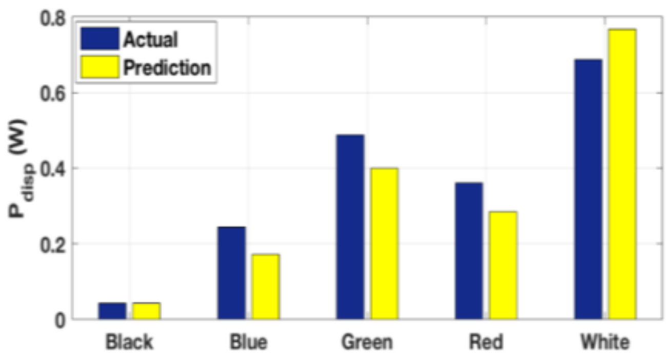
Electronics 10 02428 g004
Figure 5. Comparison of actual and predicted display power for different colors.
Electronics 10 02428 g005
Figure 6. The test image.
Electronics 10 02428 g006
Figure 7. Comparison of actual and predicted display power for the test image.
Electronics 10 02428 g007
Figure 8. Power estimation when total power is dominated by leakage of A57 cores.
Electronics 10 02428 g008
Figure 9. Reference and estimated dynamic power consumption for the A57 cluster running at 1.24 GHz.
Electronics 10 02428 g009
Figure 10. (a) Behavior of the total power of the A53 cluster running at 860 MHz as a function of the temperature. The figure shows both measured and estimated power at two configurations. (b) Behavior of the dynamic power with temperature. The dynamic power is constant since the processor is idle. (c) Behavior of the leakage power with respect to the temperature. The leakage power shows an increase with temperature due to the temperature term in Equation (5).
Electronics 10 02428 g010
Figure 11. Comparison of measured and estimated dynamic power for the A53 cluster running at 1.24 GHz. Each sample is 50 ms.
Electronics 10 02428 g011
Figure 12. Variation of power with temperature and frequency.
Electronics 10 02428 g012
Figure 13. The reference and estimated C_(dyn,gpu) at 600 MHz.
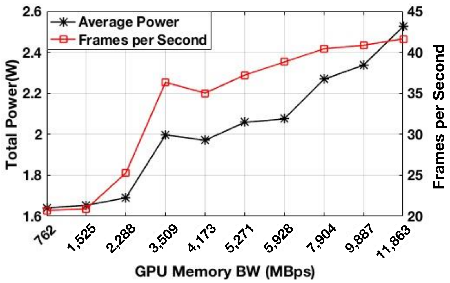
Electronics 10 02428 g013
Figure 14. Actual power consumption and average execution time of PCA benchmark for all the bandwidths.
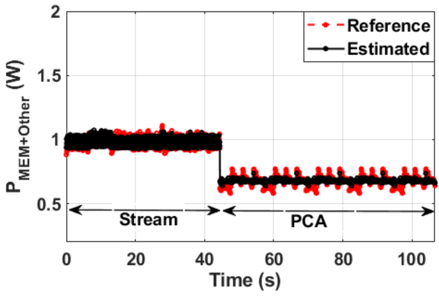
Electronics 10 02428 g014
Figure 15. Comparison of actual and predicted memory power for PCA and Stream benchmarks.
Electronics 10 02428 g015
Figure 16. Actual power consumption and execution time of the Candy Crush game for all the GPU memory bandwidths.
Electronics 10 02428 g016
Figure 18. (a). Instructions for the Angry Bird game app without alignment (b). Instructions for the Angry Bird game app with alignment of instructions.
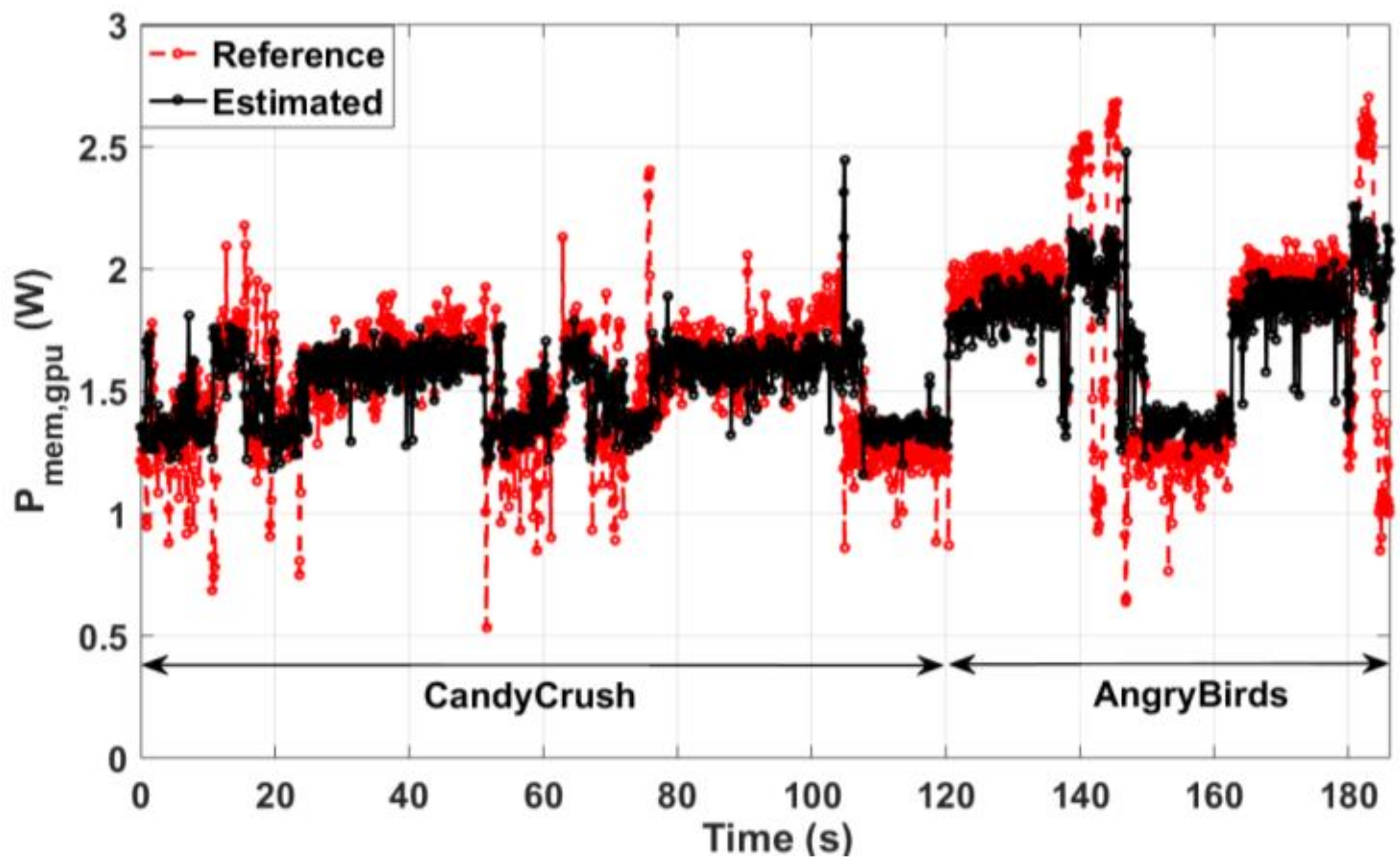
Electronics 10 02428 g018
Figure 19. Comparison of actual and predicted memory power for the Angry Birds game benchmark.
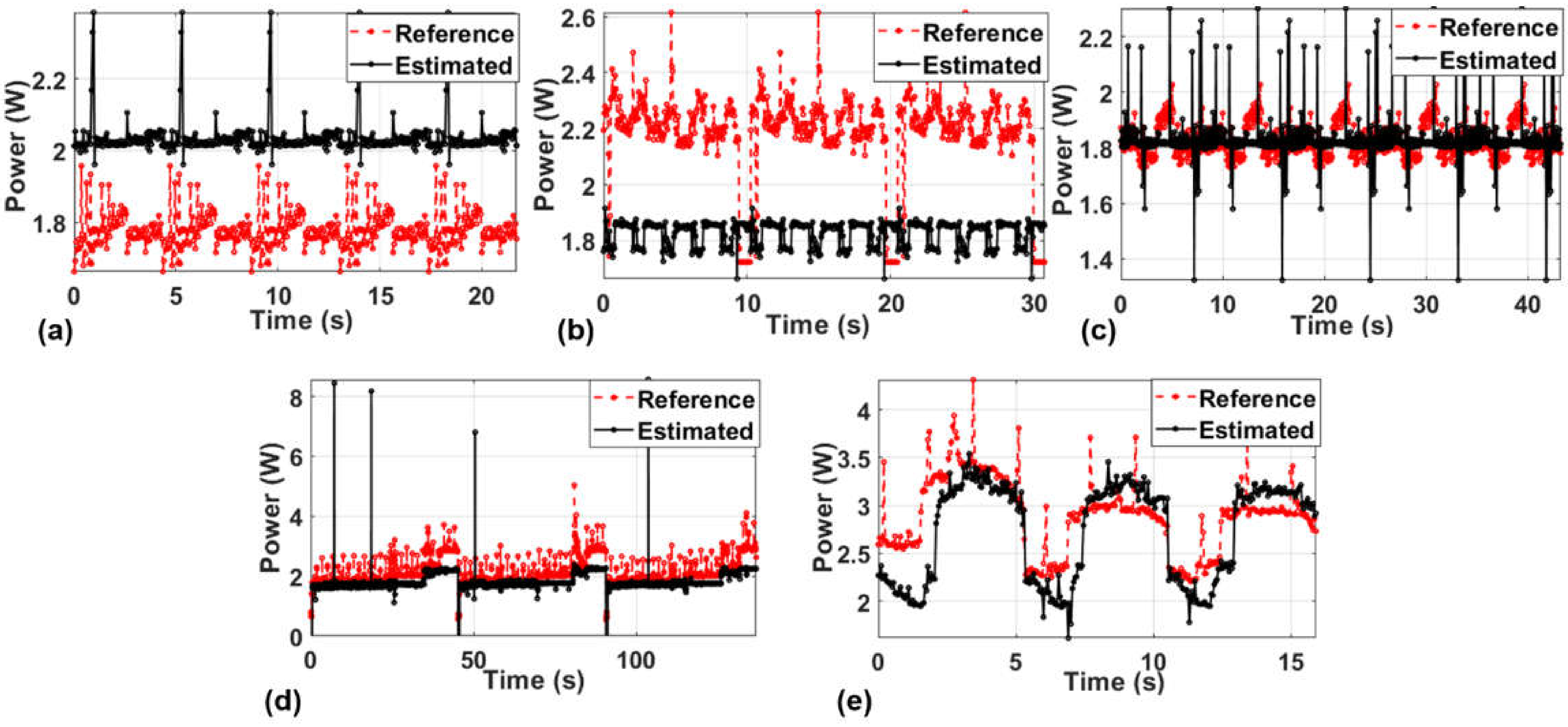
Electronics 10 02428 g019
Figure 20. Comparison of the reference power consumption and the estimated power consumption for (a) BasicMath, (b) PCA, (c) MEL, (d) FFT, and (e) Spectral benchmarks using leave-one-out analysis.
Electronics 10 02428 g020
Figure 21. (a). Wi-Fi packet transfer for an application download (b). Wi-Fi packet transfer for Google Hangouts Call.
Electronics 10 02428 g021
Figure 22. Comparison of reference and estimated power for the WiFi power.
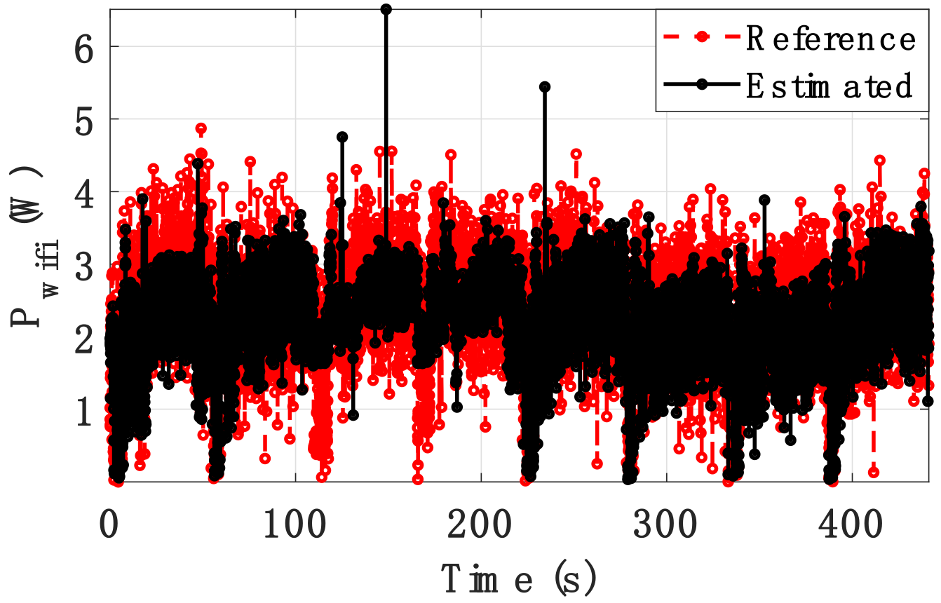
Electronics 10 02428 g022
Figure 23. Comparison of reference and estimation of the Wi-Fi power.
Electronics 10 02428 g023
Figure 24. Comparison of each power component when the WiFi is turned off randomly.
Electronics 10 02428 g024
Table 1. CPU feature selection table.
Feature IdPerformance CountersFeature IdPerformance Counters
1Aggregated Normalized Instructions6Max Utilization—U1
2CPU Cycles per Instruction72nd highest Utilization—U2
3L2 References per Instruction83rd highest Utilization—U3
4L2 Misses per Instruction94th highest Utilization—U4
5Branch misses per Instruction
Table 2. Benchmarks used in dynamic power estimation and their runtime.
BenchmarkRuntime (Approximated)
BasicMath4 s
PCA10 s
MEL10 s
Table 3. Summary of results for the A57 cluster dynamic power estimation.
BenchmarkCoreFrequency (GHz)MAPERMSEFeature Selection
PCA + MELBig1.962.70.0861 2 3 4 5 9 10
Combined 1Big1.256.40.1291 3 4 5 8 9
Combined 1Big0.388.80.27181 3 4 5 8 9 10
1 Combined = BasicMath + PCA + MEL.
Table 4. Summary of results for the A57 cluster with the union of features.
BenchmarkCoreFrequency (GHz)MAPE (Selected)MAPE (Union)
PCA + MELBig1.962.72.67
Combined 1Big1.256.46.4
Combined 1Big0.388.88.8
1 Combined = BasicMath + PCA + MEL.
Table 5. Summary of results for A53 dynamic power modeling.
BenchmarkCoreFrequency (GHz)MAPERMSEFeature Selection
Combined 1Little1.554.800.03721 2 3 4 5 8
Combined 1Little1.255.500.04391 3 4 6 7
Combined 1Little0.6011.400.12131 2 3 7 8 9
1 Combined = BasicMath + PCA + MEL.
Table 6. Summary of results with union of features.
BenchmarkCoreFrequency (GHz)MAPE (Selected)MAPE (Union)
Combined 1Little1.554.804.80
Combined 1Little1.255.505.43
Combined 1Little0.6011.4011.39
1 Combined = BasicMath + PCA + MEL.
Table 7. Leakage power parameters for the GPU.
ParameterValueParameterValue
c 1 , g p u 0.2561 a 0.1496
c 2 , g p u −3740 b 0.6003
I g a t e , g p u 8.6 × 10⁻⁸ P o t h e r 1.2985
C d y n , g p u 0.3789
Table 8. GPU feature selection table.
Feature IdPerformance CountersFeature IdPerformance Counters
1GPU Capacity7L2 Misses per Instruction
2GPU Utilization8Branch misses per Instruction
3GPU Frame Count9Max Utilization—U1
4Aggregated Normalized Instructions102nd highest Utilization—U2
5CPU Cycles per Instruction113rd highest Utilization—U3
6L2 References per Instruction124th highest Utilization—U4
Table 9. Summary of results for the GPU dynamic power model.
Frequency (MHz)MAPEMAPE (One Second Average)MAPE (Per Trace Average)Feature Selection
6008.827.044.253 4 5 6 8 9 11 12
51010.908.774.211 2 4 5 6 8 9 11 12
45013.1010.953.192 3 4 5 6 8 9 11 12
39014.6211.993.711 4 5 8 9 11 12
30518.8615.313.763 4 5 6 7 8 9 11 12
18017.4911.104.002 4 5 7 8 9 10 11
Table 10. Summary of results with the union of features for the GPU dynamic power.
Frequency (MHz)MAPEMAPE (One Second Average)MAPE (Per Trace Average)
SelectedUnionSelectedUnionSelectedUnion
6008.828.507.047.004.254.21
51010.9011.008.778.784.214.12
45013.1012.5510.9510.833.193.32
39014.6215.1411.9911.773.713.74
30518.8616.9915.3115.413.762.30
18017.4919.3411.1014.534.004.44
Table 11. CPU memory controller features.
Feature IdPerformance CountersFeature IdPerformance Counters
1Aggregated Normalized Instructions6Max Utilization—U1
2L2 References per Instruction72nd highest Utilization—U2
3Raw Memory Accesses per Instruction83rd highest Utilization—U3
4Normalized CPU Memory Bytes94th highest Utilization—U4
5CPU Memory Time
Table 12. Summary of results for the CPU memory controller power model.
Memory BandWidth (MBps)MAPEMAPE (One Second Average)MAPE (Per Trace Average)Feature Selection
15253.952.932.061 2 4 5 9
22885.083.424.081 2 4 5 7 9
35093.632.652.891 4 5 6 7 9
40662.951.830.361 4 5 6 8 9
51263.282.433.081 4 5 6 7 8 9
59282.941.952.231 4 5 6 7
79042.822.031.251 2 3 4 5 6 7 8 9
98872.901.851.651 2 4 6 7 8 9
11,8632.981.772.161 2 4 6
Table 13. Summary of results with the union of features for the CPU memory controller.
Memory Bandwidth (MBps)MAPEMAPE (One Second Average)MAPE (Per Trace Average)
SelectedUnionSelectedUnionSelectedUnion
15253.953.922.932.912.061.97
22885.085.093.423.424.084.1
35093.633.632.652.652.892.89
40662.952.951.831.830.360.36
51263.283.282.432.433.083.08
59282.942.951.951.952.232.25
79042.822.822.032.031.251.25
98872.902.901.851.851.651.65
11,8632.982.961.771.752.162.14
Table 14. GPU memory controller features.
Feature IdPerformance CountersFeature IdPerformance Counters
1Aggregated Normalized Instructions8Max Utilization—U1
2CPU Cycles per Instruction92nd highest Utilization—U2
3Raw Memory Accesses per Instruction103rd highest Utilization—U3
4Normalized CPU Memory Bytes114th highest Utilization—U4
5CPU Memory Time12GPU Capacity
6Normalized GPU Memory Bytes13GPU Utilization
7GPU Memory Time14Frames Count
Table 16. Summary of results with averaging the iterations for the GPU memory controller.
Frequency (MHz)MAPEMAPE (One Second Average)MAPE (Per Trace Average)
SelectedUnionSelectedUnionSelectedUnion
76214.0014.0210.5810.6300
152514.5714.8812.8313.0300
228818.7717.4414.6513.360.150
350914.1614.3212.4712.7100
417311.8611.109.958.940.080
52716.486.195.194.990.010
59289.429.677.557.680.060
79045.986.225.015.2200
98877.086.535.044.7700
11,8633.673.642.522.560.010
Table 17. CPU feature selection table.
Feature IdPerformance CountersFeature IdPerformance Counters
1Normalized Instructions83rd highest Utilization—U3
2CPU Cycles per Instruction94th highest Utilization—U4
3L2 References per Instruction10Normalized CPU MEM Bytes
4L2 Misses per Instruction11CPU Memory Time
5Branch misses per Instruction12CPU Cycles per MEM bytes
6Max Utilization—U113L2 References per MEM bytes
72nd highest Utilization—U214Raw Memory Accesses per MEM Bytes
Table 18. Benchmarks used for CPU and GPU power validation.
NoTraining SetTest Benchmark
1PCA + MEL + FFT + SpectralBasicMath
2BasicMath + MEL + FFT + SpectralPCA
3BasicMath + PCA + FFT + SpectralMEL
4BasicMath + PCA + MEL + SpectralFFT
5BasicMath + PCA +MEL + FFTSpectral
Table 19. Summary of results with leave-one-out experiments.
BenchmarkCoreFrequency (GHz)MAPE (Leave One out)
BasicMathBig1.2517.13
PCABig1.2510.2
MELBig1.253.3
FFTBig1.257.60
SpectralBig1.259.73
Table 20. Platform settings for Wi-Fi power modeling.
FeaturePerformance Counters
Little Core frequency1.24 GHz
GPU Frequency510 MHz
CPU Mem BW11,863 MBps
GPU Mem BW11,863 MBps
Table 21. Features used for Wi-Fi power modeling.
Feature IdPerformance CountersFeature IdPerformance Counters
1Max Utilization—U144th highest Utilization—U4
22nd highest Utilization—U25Transmitted packets
33rd highest Utilization—U36Received packets
Table 22. Training error for WiFi power model.
Error MetricPercentage Error
MAPE24.90%
MAPE (1 s Avg)11.45%
MAPE (trace Avg)6.22%
RMSE2.32%
Table 23. Summary of the estimated parameters and performance of the estimation model.
ParameterFeaturesEquation in the PaperEstimation ErrorValidatedSection
PDisplayBrightness, Proportion of color210–17%YesSection 3.1
Pleak,A57Voltage, Temperature5<1%YesSection 3.2
Pdyn,A57Union of Features in Table 37, 86%YesSection 3.2
Pleak,A53Voltage, Temperature5<1%YesSection 3.3
Pdyn,A53Union of Features in Table 67, 87%YesSection 3.3
Pleak,gpuGPU Voltage, GPU Temperature14<1%YesSection 3.4
Pdyn,gpuUnion of Features in Table 917,194%YesSection 3.4
PMEM,gpuUnion of Features in Table 12222%YesSection 3.5
PMEM,gpuUnion of Features in Table 152410%YesSection 3.5
Pwifi+otherTable 212711%YesSection 3.6
Publisher’s Note: MDPI stays neutral with regard to jurisdictional claims in published maps and institutional affiliations.

