1. Introduction
Digital twins, a concept from the industrial internet of things (IIoT) is the discipline of devising highly capable simulation models, especially those that consume streaming data from sensors to anticipate maintenance issues, impending failure of components and improving performance. Devising a simulation model of clinical behavior in front a disease, such as the classical propensity models, is much more difficult because humans are so unpredictable and engineering approaches obviously do not apply. Digital twins in healthcare systems is currently a hot topic under research [
1,
2,
3]. In this paper, work is reported to design a behavioral healthcare model for the case of lung cancer patients, which can be fed up into a decision support system [
4].
Data solutions, such as storing and processing health data to infer knowledge and to know about patients experience, lead to privacy concerns, eventually legal consequences can be claimed, hence anonymization is a keypoint in healthcare data manipulation [
5,
6]. In this context, anonymization arises as a tool to mitigate risks when gathering and massively processing personal healthcare data. This process allows identifying and shadowing sensitive information contained in documents, allowing its disclosure, hence avoiding to violate data protection rights of people and organisations that can be referenced in them [
2].
Data anonymization, as a method protecting sensitive information or the identity of the data owner, due to legal or ethical issues, is usually seen as a major problem in data analytic because it could lead to reduce so much the knowledge contained into the dataset. However, new training procedures, such as generative adversarial networks (GANs), aim at learning representations that preserve the relevant part of the information (about regular labels) while dismissing information about the private labels which correspond to the identity of a person. The success of this approach has been demonstrated in [
7], for instance. As a result of the GAN-based anonymization phase, a seedbed is obtained from the training data that allows not only to capture information from the original data avoiding privacy concerns, but to generate new synthetic information with a similar behavior to the original one. This result is currently being applied in generative applications on speech [
8], vision [
9], or natural language [
10]. In this work we want to demonstrate that it can be also applied in the health domain [
11], where data are scarce and missing values are everywhere.
It is worth noting that obtaining clinical data has a high cost and, many times, information is very limited. Therefore, many research projects have worked on developing reliable methods for data augmentation with synthetic instances. Medical knowledge implies an experience acquired through learning, detecting signs, looking for symptoms, assessing risks, until reaching a diagnosis and being able to propose a treatment indicated for each patient. However, often, physicians are unable to fully consider the large amount of data obtained from a patient and use it to make diagnostic decisions. By considering the total set of patients, even for a single disease, and generating synthetic experiences from a seedbed emerged from real patients, medical professionals can benefit from this valuable information better than buried within huge amounts of data.
The rest of this paper is structured as follows: In the next section, the available database with lung cancer patients records is introduced. Next, this database is cleaned in three steps following statistical and medical criteria. A short introduction about generative adversarial networks is also provided and it is indicated how static healthcare data are transformed into an image for GAN training easiness. Results are presented in
Section 3. It is demonstrated that synthetic samples follow a distribution similar to that of real patients. Moreover, following medical criteria, it is proven how synthetic data are correctly generated for alive or dead patients, and, among alive patients, they are very well generated depending on the severity of the illness. Finally, conclusion and discussion are provided about the work developed and the results obtained.
2. Materials and Methods
In this section, the available database of lung cancer patients employed is described. Next, cleaning and pre-processing of the database is explained in detail along three iterations. Furthermore, the generative adversarial network (GAN) methodology will be introduced. Finally, how healthcare data can be converted into images for easiness of GAN work is also presented.
2.1. Available Database
In order to perform this study it is necessary to access clinical-trials data from real lung cancer patients. It is worth noting to highlight the challenges of getting access to clinical trial datasets. After ethical approval, this research accessed to clinical data from patients of Hospital Universitario Virgen del Rocío (HUVR), a hospital situated in Seville, Spain, the main facility in the South of Spain. We were granted access to
OpenClinica [
12], a platform provided by the Junta de Andalucía, Consejería de Salud y Familias from the health service of Andalusia. It is used in HUVR to introduce and collect the information of the diagnosed lung cancer patients.
The dataset obtained, recorded in CSV (comma-separated values) format, contains the information about 887 patients diagnosed with lung cancer, and their 1542 corresponding variables, related to the visits of the patients to the hospital. These variables are classified following the same criteria of the codification of the platform OpenClinica. This web platform classifies the information of the patients in the following four categories:
These groups also have subgroups, such as family background, physical exploration or treatment for the medical record category, or chronic cough and relapse for evolution and clinical course.
From the machine learning perspective, it is a key point to know the types of variables that include the dataset in order to elaborate a good data trial for the GANs. The database contains variables in different formats:
Categorical: variables which represent clusters or categories of some kind, also known as nominal;
Quantitative: variables that represent amounts, also known as numerical;
Independent (treatment variables): variables that are manipulable in order to affect the outcome of an experiment. In the current dataset independent variables are Boolean;
Dependent (response variables): variables that represent the outcome of the experiment coming from the independent variable;
Dates.
In order to simplify the study and the use of GANs, all the nominal data will be codified as numerical data because the selected ones are ordinal categories.
2.2. Database Processing
A three steps procedure is applied in order to prepare the original database for its use with GANs.
2.2.1. First Iteration: Cleaning and Analysis of the Initial Database
Once the classification of the variables is completed in the different groups and subgroups, as mentioned before, the statistical study for each subgroup is carried out following the next steps:
Completing the dependent variables so that they contain the same information as their corresponding independent variables. In this first iteration, it remains to be decided which variables are used in the study; the independent, dependent or both ones;
Discarding variables with open response, for example ‘Observation’ variables. These variables generate many solutions and in most of the cases the response percentage is low and not representative, below 1.25% of the total data or patients’ information;
Discarding the variable data that do not indicate a duration. To calculate the duration of a record in this variable, we need both the starting and ending date. In this study, since each simulation represents static data or an instant of time, dates are not included;
Introducing the variables on a statistics software and carrying out the following statistical analysis:
Taking into account the statistical analysis, a decision is taken on whether or not a variable will be used in the study. The following criteria determines such decision:
Percentage of the response;
Type of response: open, list, Boolean, date, etc.
In this first iteration, the selection criteria is only statistical, with the aim to facilitate the decision from the health team, which will verify and decide whether the variable will remain in for the study or not, and also if the independent and dependent variables or both will be kept for the study.
After this first iteration for database cleaning, throughout the performance of the statistical analysis on the dataset given, some observations were derived, which were transferred to the health team in the hospital to take them into account when the selection of the data is to be made.
For the ‘Medical record’ category:
Location and ethnic: 91.46% of the diagnosed patients are located in Seville, Spain, and 99% belongs to the Caucasian ethnicity;
Educational level: 40% of the diagnosed patients have primary education, and 27.8% do not have studies;
Socio-economic level: 62% of the diagnosed patients comes from classes 8 and 9, which are workers; skilled in industry, construction and mining, electricians, shapers, welders, and mechanics (class 8), and laborers in industry, agriculture and construction, cleaners, ordinances and domestic employees (class 9);
Age: the mean of the diagnosed patients at the time, was 65.5 years;
Family background: on the original database the family background was classified according to the relative (grandparents, uncle, and aunt from the maternal and paternal side, parents, sisters and brothers) and the type of cancer (27 options). With the aim to simplify the data, a single variable was created which gives information about how many relatives were diagnosed with some type of cancer. The results are that 30% of the diagnosed patients do not have any relative diagnosed with some type of cancer and 36.2% with one diagnosed relative;
Toxic habits: a 95.78% of the diagnosed patients are (50.4%) or were (45.38%) smokers;
Body weight loss: the mean of the diagnosed patients is 3.2 kg;
Body mass index (BMI): the mean of the diagnosed patients is 27.93 kg/m
2, which is over the normal or healthy weight ([18.5–24.9] kg/m
2) [
13];
Body surface area (BSA): the mean of the diagnosed patients is 2.03 m
2, which is is over the normal adult average (1.9 m
2 for men and 1.6 m
2 for women) [
14];
TNM Classification: 71.38% of the diagnosed patients belong in stage III. Stages I, II, and III, mean that the cancer is present and the larger the number, the larger the tumor and the more it has spread into nearby tissues, without spreading to distant parts of the body (stage IV).
For the ‘Evolution and clinical course’ category:
Status: 41.27% of the diagnosed patients are alive, with a survival time with a mean of 21.38 months;
Relapse: 58.35% of the diagnosed patients suffer from a relapse, with a survival time with a mean of 15.94 months.
For the ‘Dosimetry’ category: In this classification, the dataset has a high percentage of answer for the following variables:
Planning treatment volume (PTV);
Clinical target volume (CTV);
Gross tumor volume (GTV);
Organs at risk: heart, oesophagus, and lungs.
For the ‘Quality of life’ category: This category is a survey with 4 possible answers and their results. The survey can be answered by indicating their value from 1 to 4, with 1 being a lot and 4 very little.
2.2.2. Second Iteration: Analysis of the Reduced Database
After a global team meeting with the participants of this project and receiving their feedback, specifically from the medical staff, a short list of variables was selected and the second iteration for cleaning the database was initiated.
This second iteration consists on the statistical analysis of the 64 variables chosen by the medical team. These variables are classified in the groups and subgroups listed in
Table 2.
Table 3 shows where these variables belong in the four principal groups.
For each variable, the following analysis of data was performed:
Classifying the type of the variable: nominal, Boolean, or numerical (see
Table 4).
Recording the detected anomalies (outliers);
For the numerical variables: checking its maximum and minimum values (range) and recording the detected outliers without removing them, as it is not recommended to remove outliers without thoughtful consideration as they might have an important value for the dataset.
For the Boolean variables:
For the nominal variables:
Moreover, for this iteration it was necessary to create a new variable indicated by the health team. This variable is Boolean and it has been generated from three existing variables (QT Induction, QT Concomitant, and QT Adyuvant), being 1 if any of the variables mentioned were 1, and, if not, 0.
2.2.3. Third Iteration: Outliers Identification
In this third iteration, the objective was to identify the actual outliers and delete them. An outlier is an observation in a dataset that lies a significant distance from other observations. These unusual observations can have a disproportionate effect on statistical analysis, such as the mean, which can lead to distorted results, and they can also negatively influence the resolution of the GANs’ simulation. Outliers can provide useful information about the data, so it is important to investigate them. In the last iteration, a boxplot for the numerical data was already displayed, which was the first step to identify the outliers graphically and visualize where they are located compared to the rest of the data.
There are two possibilities when removing the outliers: excluding all the row with the formatted cell (outlier) that represents a patient or transforming this unusual value into an empty cell, also known as a NULL value. For this iteration the second option will be used. This will reduce the amount of data and a statistical study of these data will be needed again, which will involve a recalculation of the maximum and minimum values (range) and the percentage of missing values.
2.3. Generative Adversarial Networks
Since their introduction in 2014 [
15], GANs have been a fast-moving topic and one of the most innovative ideas of this decade thanks to their outstanding usage for data augmentation [
16] and missing data [
17] problems. In this work, it is studied how using GANs in order to generate synthetic data that reproduce the features of lung cancer patients dataset. This generated machine is likely to be a very useful tool, as it will make possible to produce unlimited data with similar characteristics to the original one without compromising the privacy of the original individuals, avoiding any possible risk of leakage sensitive and private information.
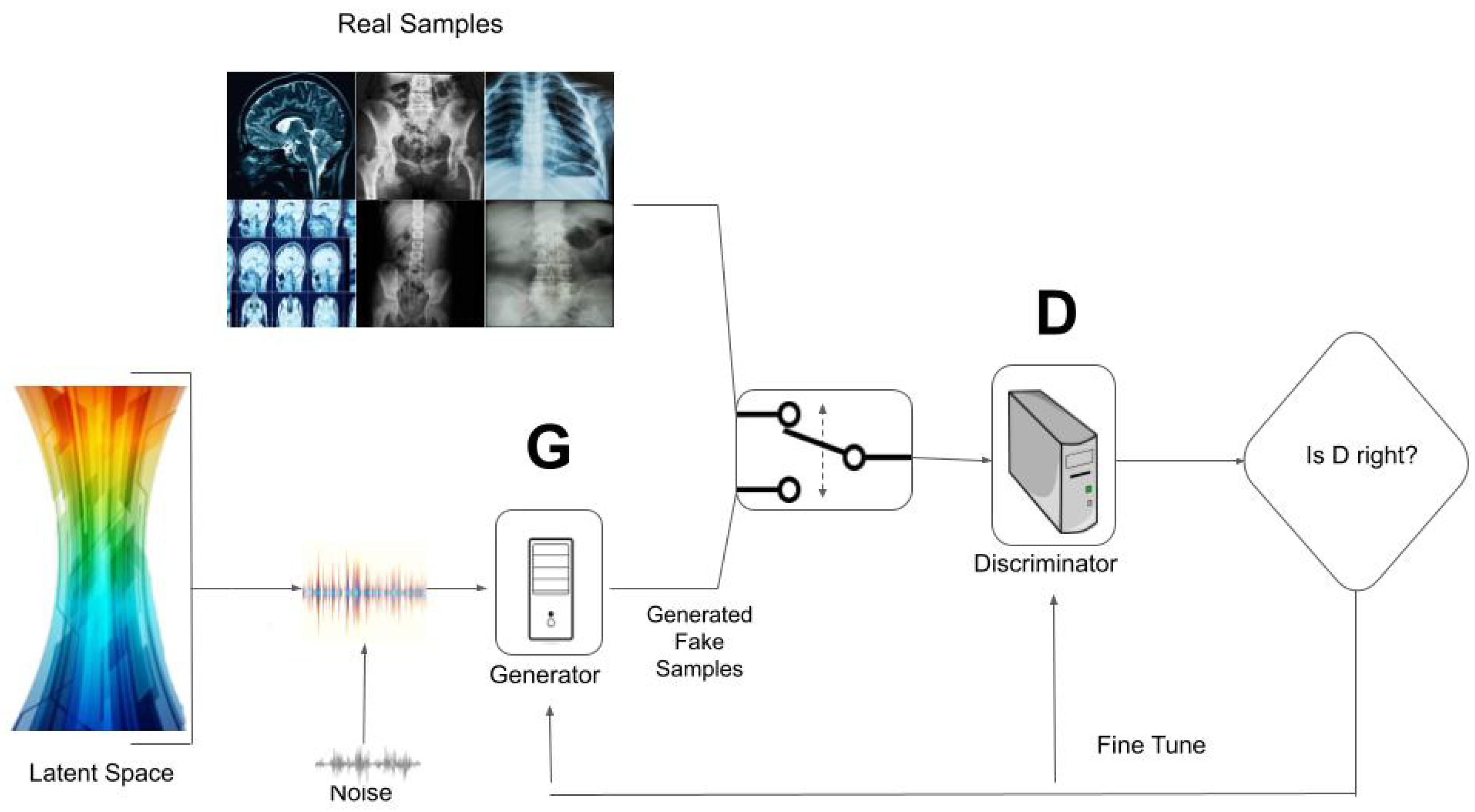
Generative adversarial networks (GANs) are a new and completely different approach on generating data because their concept is like training data. To briefly summarize how GANs work, a random sample is taken from some prior distribution, which is fed into the generator to produce some synthetic data. These fake samples along with the real data are introduced into the discriminator model, and then it decides which data come from the real dataset and which come from the fake data generated from the prior distribution.
Given a real sample (x) and some random noise vector (z), the following terms are defined:
is the output of the Discriminator when a real sample is processed;
is the output of the generator, the synthetic data;
is the prediction from the discriminator on our synthetic data;
m is the number of samples;
and are the distribution of real and noise data, respectively;
and are the expected log likelihood from the different outputs of real and generated data;
and are the weights of each model.
The expression to be considered for the complete network, discriminator and generator, is the following, and represents a value,
V,
This value function is submitted to a min-max strategy with the goal to maximize the discriminator loss and minimize the generator loss,
Value for the value function V is calculated as the sum of expected log likelihood for real or synthetic samples, and maximizing the resulting values leads to the optimization of the discriminator parameters so that it learns to correctly identify both real and fake data. A database of real samples (training data) are needed so as to distinguish between real and synthetic data.
The loss function for the discriminator is the following one:
and that for the generator is,
The most common application of GANs is the generation of realistic samples to be used in several procedures:
Data augmentation: GANs are used to generate new synthetic samples to increase the size of the original dataset;
Data anonymization: when data privacy is a critical issue, GANs are used as an anonymizing technique by replacing the original dataset with new synthetic data. The generator learns how to simulate representations that preserve the relevant part of the information;
Missing data imputation: GANs are able to generate new data, not only from scratch to increase the number of samples in a dataset, but to fill the incomplete ones;
Cross–domain transfer data: this last group of applications refers to data transformation: manipulating an input in order to get some specific results.
In particular, the healthcare industry has particularly benefited from GANs’ applications. The most common use of GANs in healthcare nowadays is in medical image synthesis [
18] and image segmentation [
19]. As it was noted in the introduction, obtaining clinical data has a high cost and sometimes the quantity of information is limited, hence, the use of GANs to generate synthetic medical data is a useful healthcare application, as it can provide strong protection for patient privacy. Usually, in medical environments, data privacy is a critical issue [
5]. This is why anonymizing techniques have been very important in data processing and analysis process, to protect sensitive information and the identification of the patient while generating a high prediction performance in their application.
2.4. Clinical-Trial Data as an Image
In 2019, a research line was initiated [
20,
21,
22] about using GANs for different medical fields. In particular it was demonstrated how data could be generated in the form of an image for databases like the Thyroid dataset, which is conformed by static data. Results were very satisfactory, as it was possible to train some stable GAN models that generated anonymous data for fake patients through GANs. This is the model that our study follows.
3. Results
Let us consider as raw dataset that obtained after the explained pre-processing. In this dataset, there are 886 patients (one patient was eliminated from the original database), with 64 features, which are normalized between 0 and 255 in order to be converted in a pixels image. Patients identification have been anonymized to preserve privacy from the starting database.
3.1. Managing Missing Values
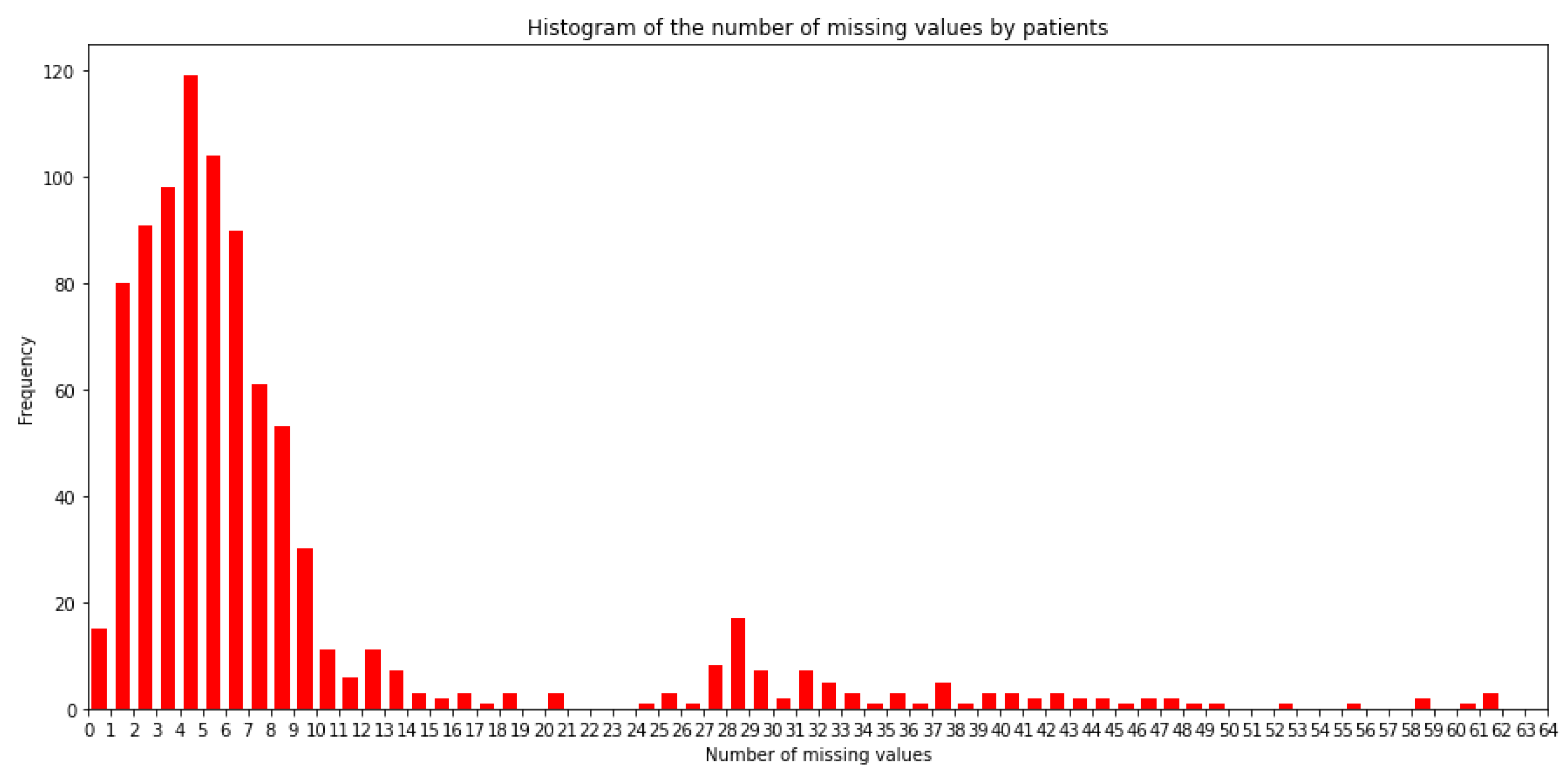
A great problem with this dataset are missing values. A value ‘0’ is assigned in the original database when a missing value is present. There exist 7230 missing values out of the 56,704 values of dataset, that is a percentage of 12.75% missing values. As the main objective is to replicate the data in the most realistic way using GANs, even absent data is considered to be replicated. Hence, it is necessary to analyze how missing values are present in the dataset.
The number of patients with missing values for each feature is depicted in the form of an histogram in
Figure 1. It can be observed that there are 15 patients of the 886 patients with all the 64 values imputed, that is, only 1.70% of the patients have a value for all the features. In the other side, there are 3 patients with only 3 values available out of the 64 possible ones.
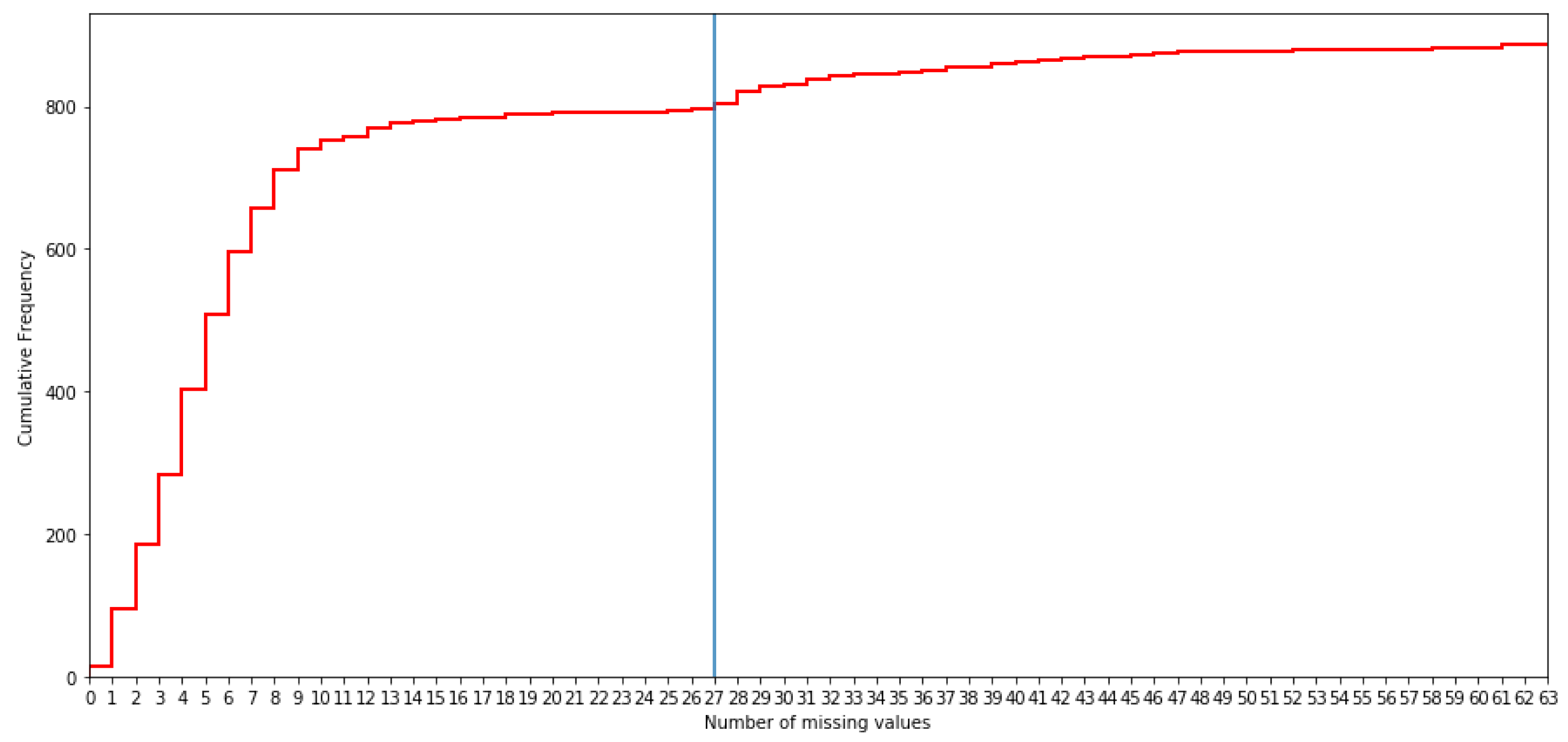
By analyzing the cumulative frequency distribution, it is decided that the maximum number of missing values allowed per patient is 21, since this is where a point of flattening is present (see
Figure 2). This decision was confirmed as a good choice by the medical team since each patient has values for more than two thirds of the variables. Let us indicate that when the medical team fills in the values of the different items in the OpenClinica software, they do not follow any standardized protocol and, therefore, it can be considered that the imputation of one variable or another depends on the dedication of the doctor to that specific patient. Therefore, if little information is taken, it indicates that the patient’s clinical history is not so relevant for the doctor.
There are 82 patients with more than 21 missing values that are not included in this study, so the cohort is conformed with 804 patients.
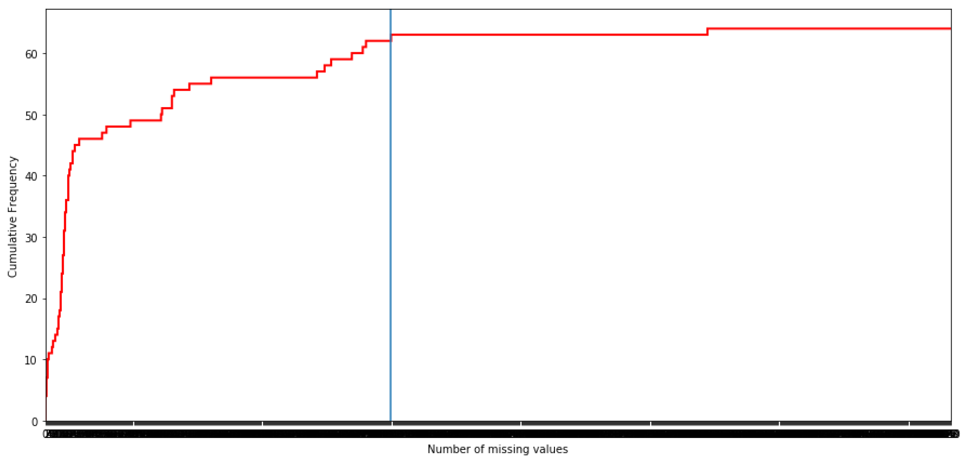
Once time the patients with more than 21 missing values are eliminated, the missing values are analyzed by features, as it can be observed in
Figure 3.
In order to see the volume of the missing values in the dataset, let us indicate that there are only four features ‘Recoded_Smoker’, ‘Hipertension’, ‘Mellitus_Diabetes’, and ‘Heart_disease’ without missing values. Hence, it is decided that the maximum number of missing values by feature is 317 since this is a point of flattening of the cumulative frequency distribution. In fact, this is a decision previously taken when the 64 features were showed to the health staff. It is worth noting that there are other points of flattening, but they are not considered because in that case several important features would be eliminated in opinion of the health staff. Both decisions are confirmed as a good choice by the medical team. Finally, there exists one feature (‘Recoded_PD_L1’) with 607 missing values which the medical team does not consider essential in the analysis and, therefore, it is eliminated.
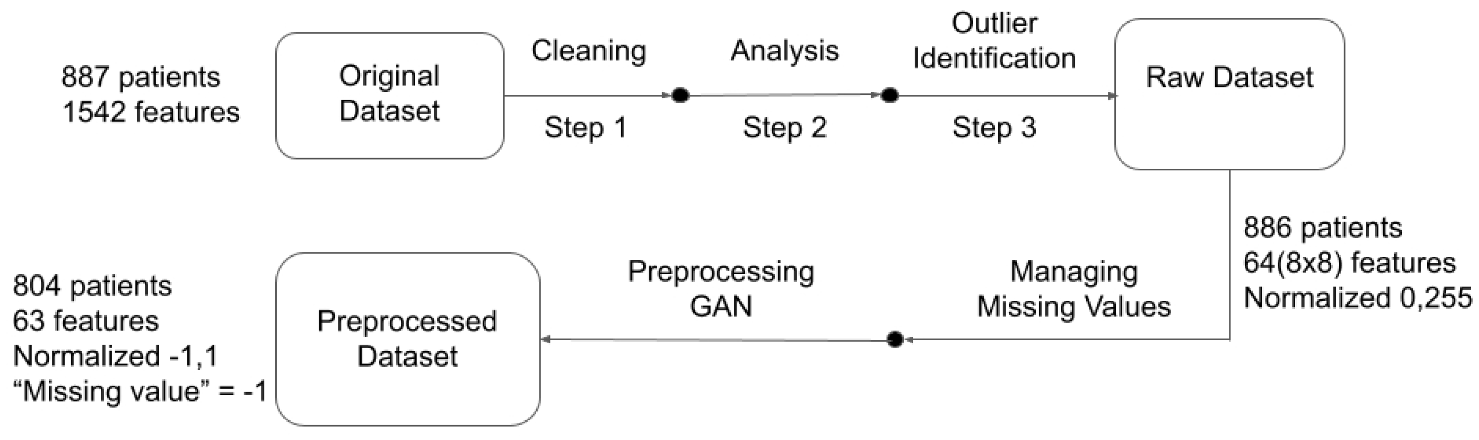
Hence, after the process of eliminating patients and features due to missing values, the dataset obtained has 804 instances from the original 886 patients (90.75%), with 63 features from 64 (98.44%), and 3597 missing values from 7230 (49.75%).
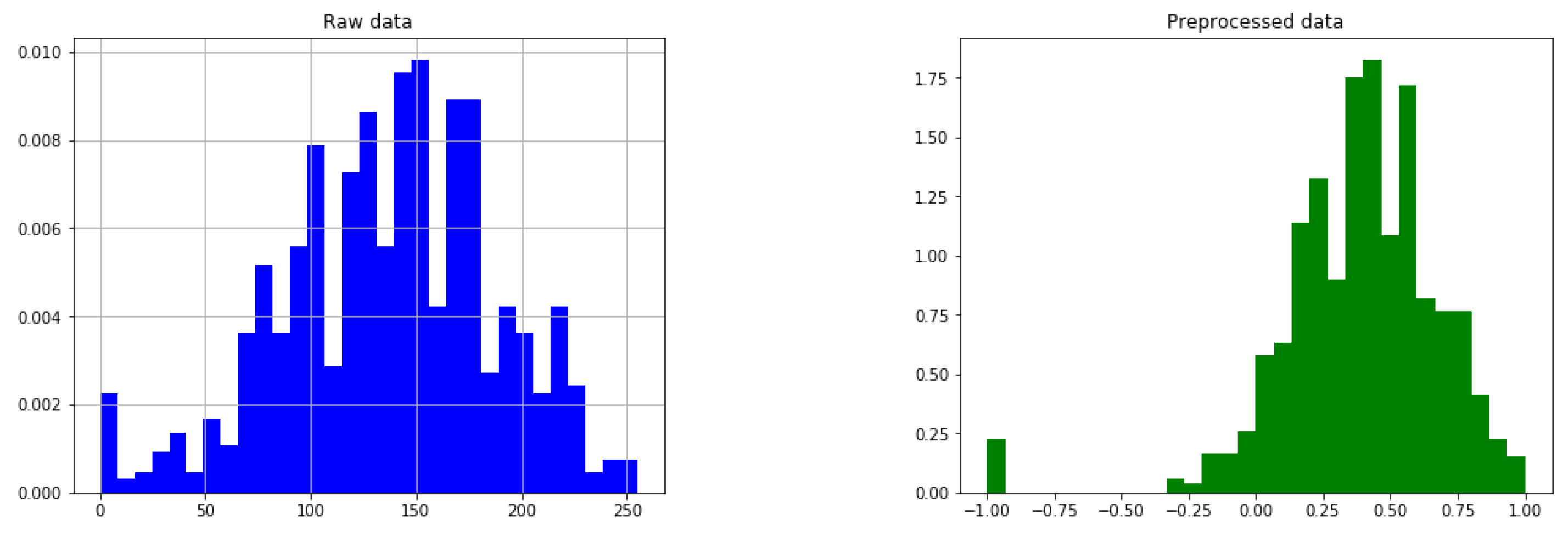
3.2. Pre-Processing Data
The range of values for all the features is [0, 255], in order to convert it in the form of a coloured pixel, where a ‘0’ value denotes that this value is missing. For ordinal data, this value is very close to the value ‘1’, which is the minimum value of the ordinal and categorical features. This value imputation confuses the network when training, so it will be moved away at a distance of 90 in the [0, 255] range. Hence, after separating the null value (‘0’ in the database) from the first value in the actual range of the feature, data are re-scaled in the range between 90 and 255 in order to generate the image. Next, it is scaled again between in the range between −1 and 1 so that they take appropriate values for the neuronal network.
An example of the pre-processing step is given in
Figure 4.
It can be observed how missing values are separated of the real ones for the ‘
Age’ feature. We rely on the network to learn how to properly handle those anomalies. In order to illustrate all the preprocessing,
Figure 5 is provided. It depicts all the preprocessing steps carried out with the data from the dataset provided by the hospital to the dataset feeding the GAN.
3.3. GAN Setup
The structure of the GAN model can be seen in
Figure 6. The discriminator module for the proposed GAN architecture is composed by five dense layers of neuronal networks (512, 256, 128, 64, and 1 neurons, respectively) all them implementing batch normalization and leaky (alpha = 0.01) layers. The generator module for the proposed GAN architecture is composed by seven dense layers (32, 1024, 512, 256, 256, 128, and 63 neurons, respectively), where the input is a noise vector of size 32 following a
uniform distribution and the output is a vector of size 63, the same as the number of features in the dataset used in the implementation. The optimizer used in both modules is Adam with a rate learning equal to
. The number of EPOCH carried out was to 2500.
Parameters have been settled to BUFFER_SIZE = 804, that is the size of the dataset, and BATCH_SIZE = 268, one third of the 804 patients. The loss function for the discriminator is based on the cross entropy and the loss for the generator is based on the mean squared error of the percentiles between real and synthetic data. Furthermore, in order to analyze the stability of the training regime, the Fréchet Inception Distance between real and synthetic data is obtained in each iteration. A threshold value equal to is also set as an early stop of the code.
3.4. GAN Implementation
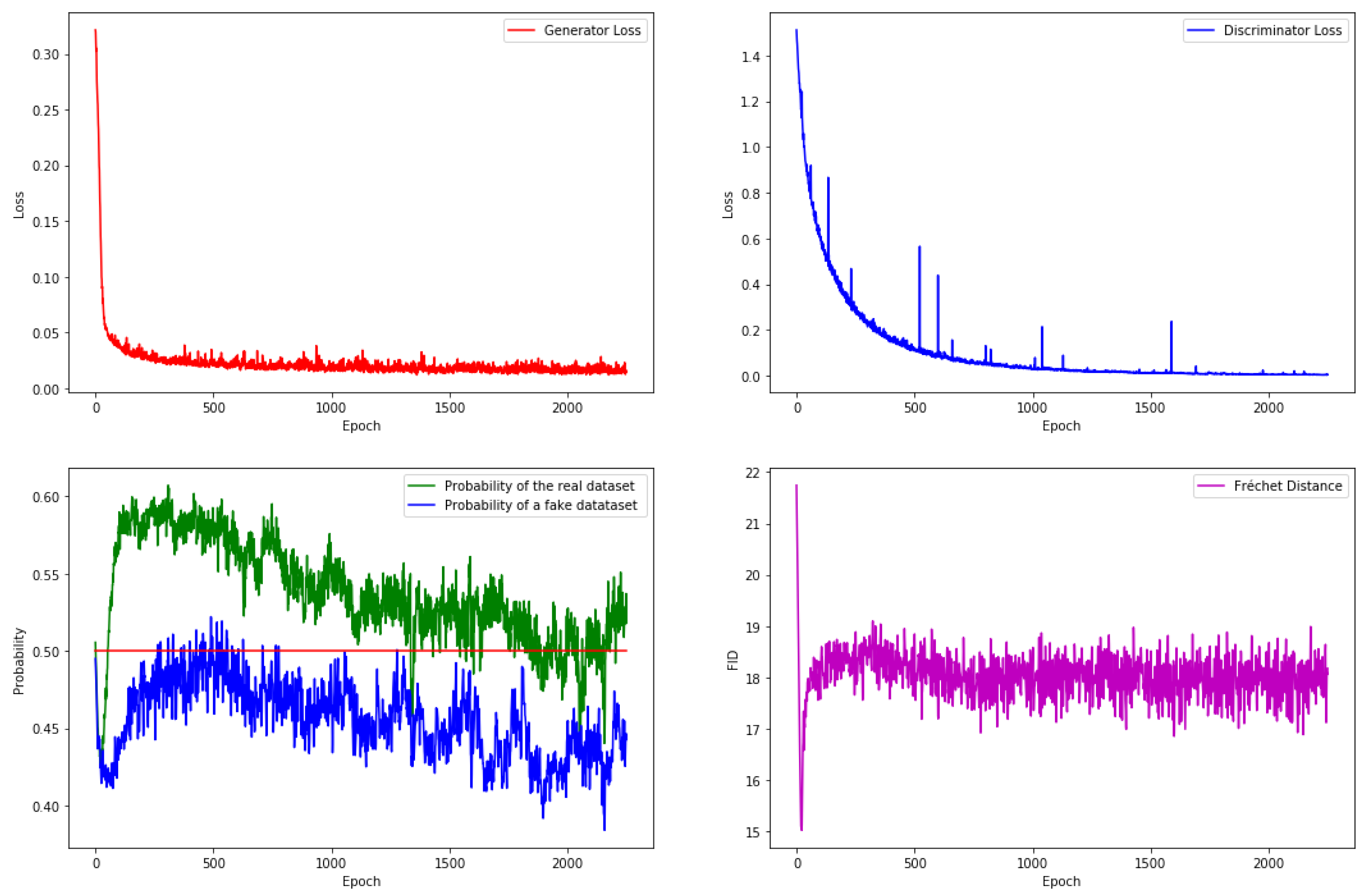
The proposed GAN is running on the database and the result for the training is shown in
Figure 7.
The upper part (left and right) shows the generator and discriminator losses, respectively. It can be observed that both losses are stable when code is finished. The lower right corner shows the Fréchet Inception Distance, which is also stabilized.
The lower left corner shows the probabilities given by the discriminator to the real and fake or synthetic data. These probabilities do not have completely stabilized, but this is not totally possible because the random generation of the batch of real data. In the ideal case, the trained GAN should provide the same probabilities by the real and fake data, that is 50%. In our experiments, a dataset of synthetic data is generated sized 30 times the amount of instances in the actual dataset. Accuracy provided by the discriminator is 50.06% for the real data and 45.40% for the fake data, that is, the results are very good since they are very close to the ideal 50%. These generated synthetic instances will be used for testing in the next development of this paper.
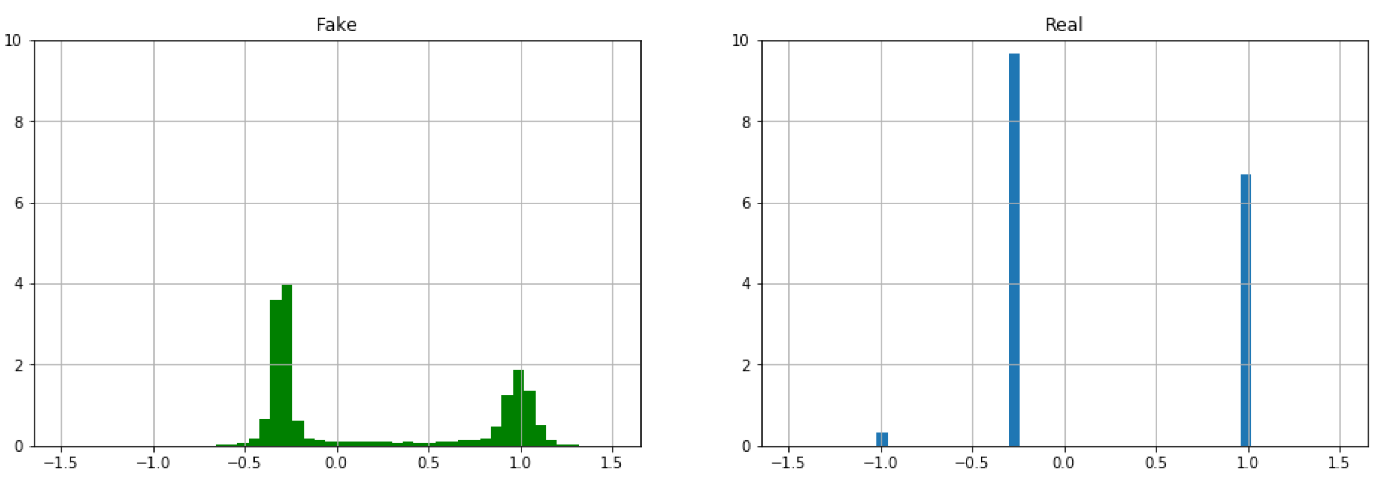
Figure 8 shows the histogram for the feature ‘
Recoded_Status’ of the generated synthetic instances (left) and real data (right). As it was expected, the GAN generated synthetic data are reproducing a similar statistical result to the original one.
This feature is Boolean. A Boolean variable has two values, usually 0 and 1, nevertheless in this paper has been considered a new value, which represent that this values is missing, taken three values: ‘−1’ (missing value), ‘−0.294118’ (dead patient) and ‘1’ (alive patient). It is very clear that the distribution of the synthetic instances is not completely similar to that of real data since the generator is a neural network that provides quantitative features. Therefore, it is necessary to carry out a post-processing for this kind of known nominal or Boolean features.
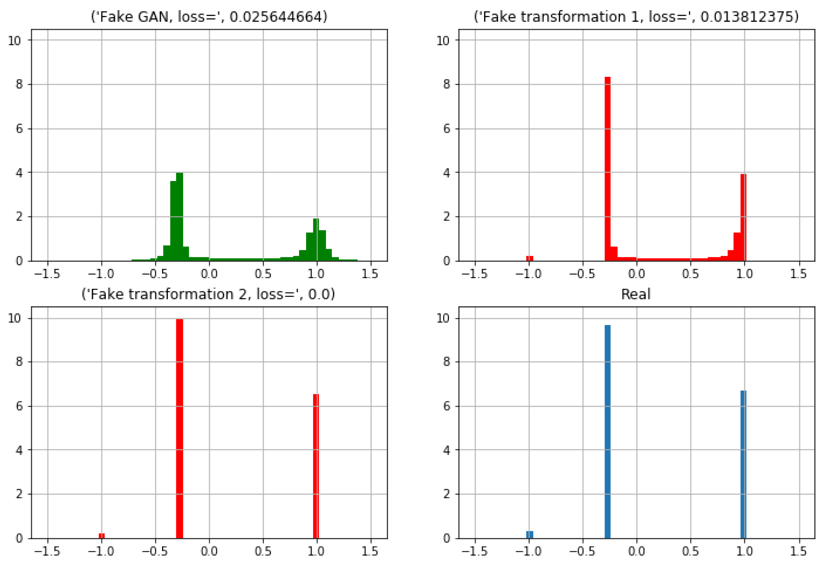
3.5. Post-Processing of GAN Generated Synthetic Data
A post-processing phase is carried out in two steps.
Figure 9 shows how this two steps transformation is applied on the ‘
Recoded_Status’ feature. On the upper left corner is depicted the histogram from the GAN generated synthetic instances. On the upper right corner the first transformation is applied and a new histogram is obtained. Finally, in the lower part it can be observed the histogram for the synthetic data after the second transformation (left) and that for the real data (right).
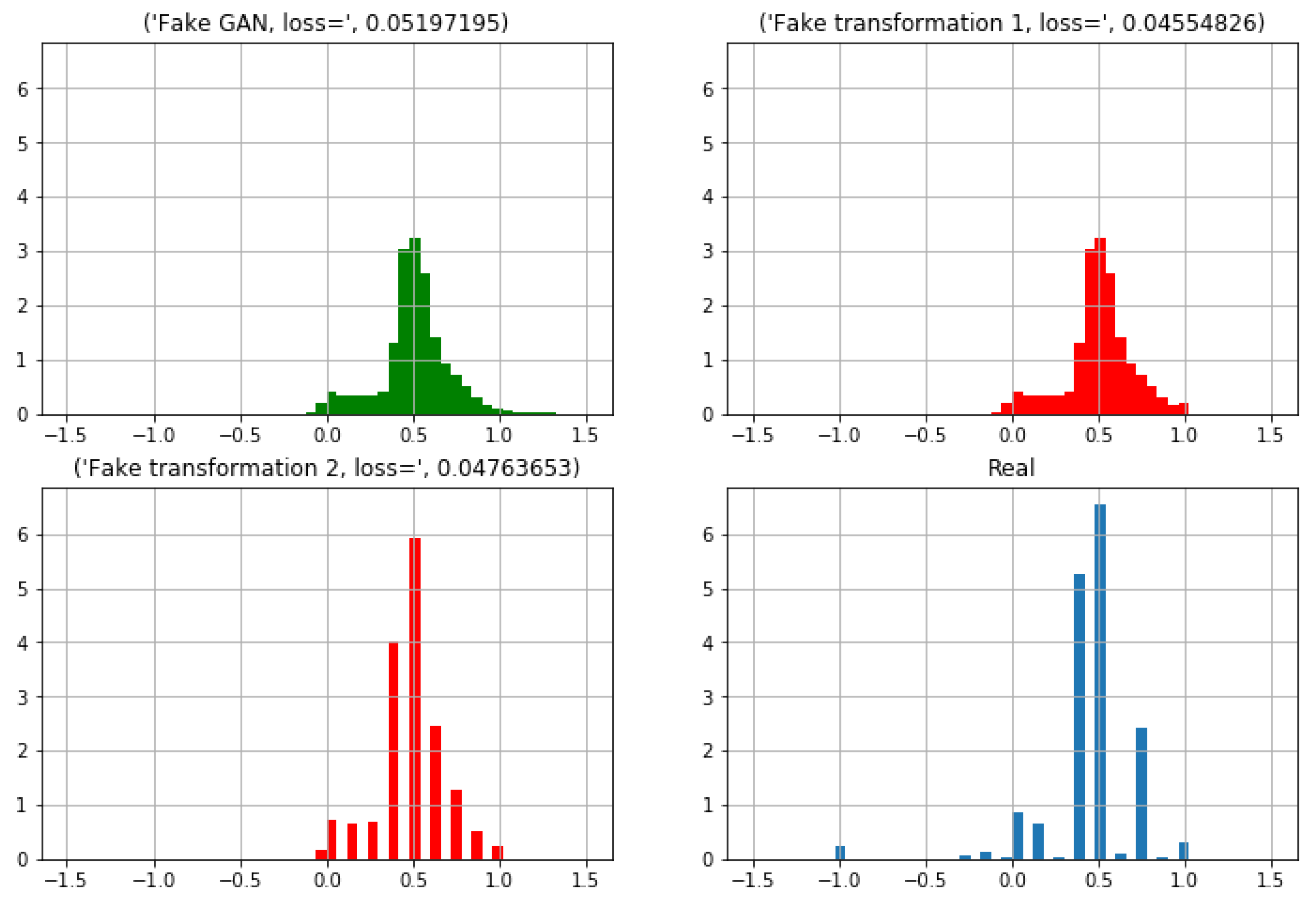
3.6. Testing the Accuracy of the Synthetic Data
In order to validate whether the distribution of the synthetic data can be considered similar to the real patients, health staff indicates that ‘Recoded_Status’ and ‘Recoded_Clinical_ Stage’ features should be considered. As previously explained the first feature corresponds to determine whether a patient is alive. The second considered feature corresponds to the severity of the lung cancer.
Similarly to the two steps transformation completed for the first feature (‘
Recoded_Status’), was also performed for ‘
Recoded_Clinical_Stage’. The distribution for this latter feature can be observed in
Figure 10. It can be noted as the fitting between the real distribution and the synthetic data distribution are increasingly similar, although it is not the same.
A summary of the statistics for these two features is provided in
Table 5.
Now, the loss function employed for the generator (mean squared error of 20 percentiles between real and synthetic data) will be also used in order to provide a measure of the fitting between the distribution of the real data and and the corresponding distribution to the synthetic data. For the
Recoded_Status feature, results are provided in
Table 6. It can be observed that the synthetic instances provided by the GAN are excellent from this point of view. The difference between real and synthetic samples is only 1.02% according to the 20 percentiles loos function.
With respect to the ‘
Recoded_Clinical_Stage’ feature, medical staff indicated that stages IIIA, IIIB, and IV are the most important ones when taking also into account the ‘
Recoded_Satatus’ feature. Hence,
Table 7 is presented.
In this table, it can be observed that, again, results are excellent for the case of alive patients. Difference is in all the cases lower than 2%. However, results for dead patient are no so impressive, with an error rate between 6% and 15%.
4. Conclusions and Discussion
High quality synthetic health data are a valuable resource for anonymization of healthcare records in the form of a digital twin. In this paper, it has been demonstrated that using a generative adversarial network on images translating information from lung cancer patients it is possible to capture relationships across the various features in real patients. Hence, the presented results show that it is possible to use these synthetic data to generate models for digital twins since they collect the fundamental characteristics of the real data. Moreover, by using these kind of synthetic data in the design and construction of the lung cancer disease modeling ensures that the privacy of the subjects included in the real data is not disclosed and the number of data that it generates can be of the size that the researchers team requires for his study.
Furthermore, the existence of many missing values in a database is a great challenge in any area of knowledge and, in particular, in machine learning. The usual practice is to fill in these missing values following some procedure or tool. The data obtained after a medical check-up usually present many missing values. Therefore, a very important point in our approach has been to work directly with a database of real patients with lung cancer where the number of missing values is large and to obtain such a quality in the synthetic data that, in the opinion of the medical team, it is acceptable.
The presented study shows excellent results for variables that medical staff consider as the key ones, related with the mortality of the patients and the severity of the illness. Although there is some path for improvement, we believe that results provide a novel and interesting approach for the generation of synthetic data in the healthcare domain. We provided a detailed explanation of the novel technology and hope that it can be helpful in guiding researchers in generating synthetic data for their specific application.
The introduced work leads to a very useful tool as it is enabling unlimited similar-to-the-original data without compromising the privacy of the original elements. The applications of this tool range from educational purposes with young health professionals [
23] to scientific simulations and investigations using synthetic signals for the training of automatic systems for the detection of diseases.
The study carried out in this paper is a novel approach to the generation of systematic data in the healthcare domain, hence a number of limitations is still present. For instance, not all the variables from the original database have been used, only a selection of them, according to medical professionals advice. This selection has probably biased the problem and some correlations that could have been obtained from the original data cannot be maintained into the synthetic data.
Author Contributions
Conceptualization, L.G.-A. and C.A.; methodology, L.G.-A. and J.-L.L.-G.; software, L.G.-A., C.A., and J.-A.O.; validation, L.G.-A. and J.-L.L.-G.; formal analysis, J.-L.L.-G.; investigation, L.G.-A. and C.A.; resources, J.-L.L.-G. and J.-A.O.; data curation, L.G.-A. and J.-L.L.-G.; writing—original draft preparation, L.G.-A. and C.A.; writing—review and editing, C.A., J.-A.O., and J.-L.L.-G.; visualization, L.G.-A.; supervision, J.-L.L.-G.; project administration, J.-A.O.; funding acquisition, L.G.-A., C.A., and J.-A.O. All authors have read and agreed to the published version of the manuscript.
Funding
This research was partly funded by the Spanish Ministry of Science, Innovation and Universities (AEI/FEDER, UE) grant numbers PGC2018-102145-B-C21 and PGC2018-102145-B-C22 (research project EDITH). Cecilio Angulo has been partly supported by the European Union’s Horizon 2020 research and innovation programme under grant agreement No. 825619 (AI4EU).
Institutional Review Board Statement
The study was conducted according to the guidelines of the Declaration of Helsinki, and approved by the Ethics Committee Comité Coordinador de Ética de la Investigación Biomédica de Andalucía (protocol code 2282-N-20 and date 27 April 2021).
Informed Consent Statement
Not applicable.
Data Availability Statement
The data presented in this study are available on request from the corresponding author. The data are not publicly available due to ethical restrictions.
Acknowledgments
We want acknowledge technical support given by Sara González García (Hospital Universitario Virgen del Rocío), José Mariano González Romano (Universidad de Sevilla), and Maria del Mar Espinàs Salla (Universitat Politècnica de Catalunya).
Conflicts of Interest
The authors declare no conflict of interest. The funders had no role in the design of the study; in the collection, analyses, or interpretation of data; in the writing of the manuscript, or in the decision to publish the results.
References
- Elayan, H.; Aloqaily, M.; Guizani, M. Digital Twin for Intelligent Context-Aware IoT Healthcare Systems. IEEE Internet Things J. 2021. [Google Scholar] [CrossRef]
- Angulo, C.; Gonzalez-Abril, L.; Raya, C.; Ortega, J.A. A Proposal to Evolving Towards Digital Twins in Healthcare. In Bioinformatics and Biomedical Engineering; Rojas, I., Valenzuela, O., Rojas, F., Herrera, L.J., Ortuño, F., Eds.; Springer International Publishing: Cham, Switzerland, 2020; pp. 418–426. [Google Scholar]
- Rivera, L.F.; Jiménez, M.; Angara, P.; Villegas, N.M.; Tamura, G.; Müller, H.A. Towards Continuous Monitoring in Personalized Healthcare through Digital Twins. In Proceedings of the 29th Annual International Conference on Computer Science and Software Engineering (CASCON ’19), Markham, ON, Canada, 4–6 November 2019; pp. 329–335. [Google Scholar]
- Angulo, C.; Ortega, J.A.; Gonzalez-Abril, L. Towards a Healthcare Digital Twin. In Frontiers in Artificial Intelligence and Applications; Sabater-Mir, J., Torra, V., Aguiló, I., González-Hidalgo, M., Eds.; IOS Press: Oxford, UK, 2019; Volume 319, pp. 312–315. [Google Scholar]
- Bae, H.; Jung, D.; Yoon, S. AnomiGAN: Generative Adversarial Networks for Anonymizing Private Medical Data. 2019. Available online: http://www.lanl.gov/abs/1901.11313 (accessed on 10 September 2021).
- Bruynseels, K.; Santoni de Sio, F.; van den Hoven, J. Digital Twins in Health Care: Ethical Implications of an Emerging Engineering Paradigm. Front. Genet. 2018, 9, 31. [Google Scholar] [CrossRef] [PubMed]
- Piacentino, E.; Angulo, C. Anonymizing Personal Images Using Generative Adversarial Networks. In Bioinformatics and Biomedical Engineering; Rojas, I., Valenzuela, O., Rojas, F., Herrera, L.J., Ortuño, F., Eds.; Springer International Publishing: Cham, Switzerland, 2020; pp. 395–405. [Google Scholar]
- Phan, H.; McLoughlin, I.V.; Pham, L.; Chen, O.Y.; Koch, P.; De Vos, M.; Mertins, A. Improving GANs for Speech Enhancement. IEEE Signal Process. Lett. 2020, 27, 1700–1704. [Google Scholar] [CrossRef]
- Wang, Z.; She, Q.; Ward, T.E. Generative Adversarial Networks in Computer Vision: A Survey and Taxonomy. 2020. Available online: http://www.lanl.gov/abs/1906.01529 (accessed on 10 September 2021).
- Zhu, Y.; Zhang, Y.; Yang, H.; Wang, F. GANCoder: An Automatic Natural Language-to-Programming Language Translation Approach based on GAN. 2019. Available online: http://www.lanl.gov/abs/1912.00609 (accessed on 10 September 2021).
- Piacentino, E.; Angulo, C. Generating Fake Data. In Bioinformatics and Biomedical Engineering; Rojas, I., Valenzuela, O., Rojas, F., Herrera, L.J., Ortuño, F., Eds.; Springer International Publishing: Cham, Switzerland, 2020; pp. 406–417. [Google Scholar]
- Cavelaars, M.; Rousseau, J.; Parlayan, C.; de Ridder, S.; Verburg, A.; Ross, R.; Visser, G.; Rotte, A.; Azevedo, R.; Boiten, J.; et al. OpenClinica. J. Clin. Bioinform. 2015, 5, S2. [Google Scholar] [CrossRef] [Green Version]
- U.S. Department of Health & Human Services; Centers for Disease Control and Prevention. About Adult BMI. September 2020. [Google Scholar]
- Conrad-Stöppler, M. Medical Definition of Body surface area. December 2018. Available online: https://www.medicinenet.com/body_surface_area/definition.htm (accessed on 10 September 2021).
- Goodfellow, I.; Pouget-Abadie, J.; Mirza, M.; Xu, B.; Warde-Farley, D.; Ozair, S.; Courville, A.; Bengio, Y. Generative Adversarial Nets. Adv. Neural Inf. Process. Syst. 2014, 27, 2672–2680. [Google Scholar]
- Connor, S.; Taghi, M.K. A survey on Image Data Augmentation for Deep Learning. J. Big Data 2019, 6, 60. [Google Scholar] [CrossRef]
- Yoon, J.; Jordon, J.; van der Schaar, M. GAIN: Missing Data Imputation using Generative Adversarial Nets. 2018. Available online: http://www.lanl.gov/abs/1806.02920 (accessed on 10 September 2021).
- Skandarani, Y.; Jodoin, P.M.; Lalande, A. GANs for Medical Image Synthesis: An Empirical Study. 2021. Available online: http://www.lanl.gov/abs/2105.05318 (accessed on 10 September 2021).
- Yi, X.; Walia, E.; Babyn, P. Generative adversarial network in medical imaging: A review. Med. Image Anal. 2019, 58, 101552. [Google Scholar] [CrossRef] [PubMed] [Green Version]
- Piacentino, E. Generative Adversarial Network Based Machine for Fake Data Generation. Master’s Thesis, Universitat Politècnica de Catalunya, Barcelona, Spain, 2019. [Google Scholar]
- Guarner, A. Using GANs to Generate Fake Patients. Master’s Thesis, Universitat Politècnica de Catalunya, Barcelona, Spain, 2020. [Google Scholar]
- Piacentino, E.; Guarner, A.; Angulo, C. Generating Synthetic ECGs Using GANs for Anonymizing Healthcare Data. Electronics 2021, 10, 389. [Google Scholar] [CrossRef]
- Goncalves, A.; Ray, P.; Soper, B.; Stevens, J.; Coyle, L.; Sales, A.P. Generation and evaluation of synthetic patient data. BMC Med. Res. Methodol. 2020, 20, 108. [Google Scholar] [CrossRef] [PubMed]
Figure 1.
Histogram of the number of missing values by patients.
Figure 1.
Histogram of the number of missing values by patients.
Figure 2.
Cumulative histogram of the number of missing values by patients.
Figure 2.
Cumulative histogram of the number of missing values by patients.
Figure 3.
Cumulative histogram of the number of missing values by features.
Figure 3.
Cumulative histogram of the number of missing values by features.
Figure 4.
Histogram of the ‘Age’ feature before (when normalized in the range 0 to 255 for the image generation) and after pre-processing.
Figure 4.
Histogram of the ‘Age’ feature before (when normalized in the range 0 to 255 for the image generation) and after pre-processing.
Figure 5.
Representation of the total preprocessing carried out from the original dataset to the one employed to feed the GANs.
Figure 5.
Representation of the total preprocessing carried out from the original dataset to the one employed to feed the GANs.
Figure 6.
Structure of the GAN model.
Figure 6.
Structure of the GAN model.
Figure 7.
Training results for the implemented GAN architecture. Losses (upper part), Accuracy on real and synthetic data (lower left), and Fréchet distance (lower right) are depicted.
Figure 7.
Training results for the implemented GAN architecture. Losses (upper part), Accuracy on real and synthetic data (lower left), and Fréchet distance (lower right) are depicted.
Figure 8.
Distribution of the values for the ‘Recorded_Status’ feature for the synthetic (left) and real (right) data.
Figure 8.
Distribution of the values for the ‘Recorded_Status’ feature for the synthetic (left) and real (right) data.
Figure 9.
Distribution of the ‘Recoded_Status’ feature from the raw GAN-generated synthetic data (upper left), after the first (upper right) and the second transformation (lower left) and that from the real patients (lower right).
Figure 9.
Distribution of the ‘Recoded_Status’ feature from the raw GAN-generated synthetic data (upper left), after the first (upper right) and the second transformation (lower left) and that from the real patients (lower right).
Figure 10.
Distribution of the ‘Recoded_Clinical_Stage’ feature from the raw GAN-generated synthetic data (upper left), after the first (upper right) and the second transformation (lower left) and that from the real patients (lower right).
Figure 10.
Distribution of the ‘Recoded_Clinical_Stage’ feature from the raw GAN-generated synthetic data (upper left), after the first (upper right) and the second transformation (lower left) and that from the real patients (lower right).
Table 1.
Descriptive statistical study of variables for the subcategory pulmonary function testing (PFT). The number of instances is 887, N representing the number of instances with known data and the number of instances with missing data ( = 887). SE Mean and StDev are the mean deviation and standard deviation of the feature, respectively.
| Variable | N | N* | Mean | SE Mean | St Dev | Min | Max |
|---|
| FEV1_porc_FVC_E2_C5 | 704 | 183 | 25.460 | 1.2400 | 33.000 | 0.0000 | 98.110 |
| PIF_E2_C5PIF_E2_C5 | 645 | 242 | 1.0460 | 0.0650 | 1.6507 | 0.0000 | 8.3200 |
| FVC_E2_C5PIF_E2_C5 | 704 | 183 | 1.1631 | 0.0595 | 1.5777 | 0.0001 | 6.5100 |
| PIF50_E2_C5PIF_E2_C5 | 618 | 269 | 0.8965 | 0.0616 | 1.5324 | 0.0002 | 8.0600 |
| DLCOc_VA_E2_C5 | 679 | 208 | 0.3881 | 0.0206 | 0.5376 | 0.0003 | 1.7400 |
| MEF50_E2_C5 | 646 | 241 | 0.5839 | 0.0417 | 1.0599 | 0.0004 | 6.3000 |
| DLCOc_SB_E2_C5 | 683 | 204 | 1.8267 | 0.0986 | 2.5756 | 0.0005 | 9.2300 |
| DLCO_SB_E2_C5 | 683 | 204 | 1.7339 | 0.0937 | 2.4476 | 0.0006 | 8.5900 |
Table 2.
List of selected variables with their corresponding number.
Table 2.
List of selected variables with their corresponding number.
| No. | Variable | No. | Variable |
|---|
| 1 | Level of studies | 33 | Primary survival rate |
| 2 | Socio-economic status | 34 | Primary-free survival |
| 3 | Age | 35 | Relapse |
| 4 | Number of Family History with cancer | 36 | PTV (planning target volume) Volume cc |
| 5 | Intention | 37 | PTV (planning target volume) Median |
| 6 | Smoker | 38 | Heart Mean |
| 7 | Alcoholism | 39 | Heart v25 |
| 8 | Hypertension | 40 | Global health status |
| 9 | Diabetes mellitus | 41 | Physical functioning |
| 10 | Dyslipidemia | 42 | Role functioning |
| 11 | Cardiovascular disease | 43 | Emotional functioning |
| 12 | Thrombosis | 44 | Cognitive functioning |
| 13 | Chronic obstructive pulmonary disease (COPD) | 45 | Social functioning |
| 14 | Weight loss | 46 | Fatigue |
| 15 | Karnofsky Performance Status (KPS) | 47 | Nausea and vomiting |
| 16 | Body mass index (BMI) | 48 | Pain |
| 17 | Body surface area (BSA) | 49 | Dyspnoea |
| 18 | Clinical stage | 50 | Insomnia |
| 19 | Histology | 51 | Appetite loss |
| 20 | Estimated Glomerular Filtration Rate (EGFR) | 52 | Constipation |
| 21 | Anaplastic lymphoma kinase (ALK) | 53 | Diarrhoea |
| 22 | Programmed death-ligand 1 (PD-L1) | 54 | Financial difficulties |
| 23 | Maximum diameter of the primary tumor | 55 | Dyspnoea lung |
| 24 | Primary tumor SUV (Standarized Uptake Value) | 56 | Coughing |
| 25 | Surgery | 57 | Haemoptysis |
| 26 | Type of surgery | 58 | Sore mouth |
| 27 | RT Pulmonary | 59 | Dysphagia |
| 28 | Administered dose | 60 | Peripheral neuropathy |
| 29 | Administered fractionation | 61 | Alopecia |
| 30 | Concomitant chemotherapy | 62 | Pain in chest |
| 31 | Induction, concomitant and adjuvant chemotherapy | 63 | Pain in arm or shoulder |
| 32 | Status | 64 | Pain in other parts |
Table 3.
The 64 variables chosen by the medical team, classified in their principal categories.
Table 3.
The 64 variables chosen by the medical team, classified in their principal categories.
| Group | Number of Variables |
|---|
| Medical record | 31 |
| Evolution and clinical course | 4 |
| Dosimetry | 4 |
| Quality of life | 25 |
Table 4.
The group of 64 variables chosen classified by their type.
Table 4.
The group of 64 variables chosen classified by their type.
| Type of Variable | Number of Variables |
|---|
| Nominal | 13 |
| Boolean | 13 |
| Numerical | 38 |
Table 5.
A summary of the statistics of the ‘Recoded_Status’ and ‘Recoded_Clinical_Stage’ features.
Table 5.
A summary of the statistics of the ‘Recoded_Status’ and ‘Recoded_Clinical_Stage’ features.
| | Recoded_Status | Recoded_Clinical_Stage |
|---|
# Different
Values | 3 | 13 |
|---|
| | Real | Synthetic | Real | Synthetic |
| count | 804 | 24,120 | 804 | 24,120 |
| # missings | 15 | 300 | 11 | 0 |
| mean | 0.211004 | 0.205637 | 0.469838 | 0.504768 |
| std | 0.652233 | 0.643817 | 0.261863 | 0.191975 |
| min | −1.000000 | −1.000000 | −1.000000 | −0.059750 |
| 25% | −0.294118 | −0.294118 | 0.414081 | 0.414081 |
| 50% | −0.294118 | −0.294118 | 0.531264 | 0.531264 |
| 75% | 1.000000 | 1.000000 | 0.531264 | 0.648448 |
| max | 1.000000 | 1.000000 | 1.000000 | 1.000000 |
Table 6.
Results of the ‘Recoded_Status’ features. In parentheses the number of dead or alive patients, that is, without counting the missing values.
Table 6.
Results of the ‘Recoded_Status’ features. In parentheses the number of dead or alive patients, that is, without counting the missing values.
| Patients | Real (789) | Synthetic (23,820) | Difference |
|---|
| Dead | 467 | 59.19% | 14342 | 60.21% | 1.02% |
| Alive | 322 | 40.82% | 9478 | 39.79% | 1.02% |
Table 7.
Results of the ‘Recorded_Clinical_Stage’ feature related with ‘Recorded_Status’ features.
Table 7.
Results of the ‘Recorded_Clinical_Stage’ feature related with ‘Recorded_Status’ features.
Dead
Patients | Real (467) | Fake (14,342) | |
|
‘Clinical_Stage’
| # | % | # | % | Difference |
| IIIA | 145 | 31.05% | 2266 | 15.86% | 15.24% |
| IIIB | 191 | 40.90% | 4993 | 34.81% | 06.09% |
| IV | 085 | 18.20% | 1149 | 08.01% | 10.19% |
Alive
Patients | Real (322) | Fake (9478) | |
|
‘Clinical_Stage’
| # | % | # | % | Difference |
| IIIA | 107 | 33.23% | 3284 | 34.68% | 1.42% |
| IIIB | 121 | 37.58% | 3524 | 37.18% | 0.40% |
| IV | 029 | 09.91% | 0676 | 07.13% | 1.87% |
| Publisher’s Note: MDPI stays neutral with regard to jurisdictional claims in published maps and institutional affiliations. |
© 2021 by the authors. Licensee MDPI, Basel, Switzerland. This article is an open access article distributed under the terms and conditions of the Creative Commons Attribution (CC BY) license (https://creativecommons.org/licenses/by/4.0/).


