1. Introduction
In recent years, Unmanned Aerial Vehicles (UAVs) have gained a massive popularity around the globe. The current technological advances have made it possible to equip these vehicles with a variety of state-of-the-art technologies such as machine vision, global position systems or a simple video camera, and so forth. Moreover, these machines are becoming widely popular over other platforms such as aircraft or helicopters due to their flight characteristics. Planes, despite being excellent flying platforms, are not effective for flights operated indoors as they are difficult to maneuver in confined spaces. On the other hand, helicopters offer great mobility in all the environments but certainly are quite difficult to control. Furthermore, helicopters may not be an appropriate mode of flying when considering indoor flights due to their fast-rotating propellers. These reasons make quadcopters an excellent alternative for indoor flights. However, the design and control of quadcopters pose a number of challenges: the multivariate system makes modelling a difficult task; the existence of coupled variables makes it difficult to control the plant; the drone must operate in a three-dimensional environment with unplanned disturbances; the need for achieving a stable system with a high degree of precision and accuracy to allow the implementation of different technologies such as artificial vision, and so forth.
A quadcopter is a machine that can fly without a pilot but in order to realize this, an implementation of a reliable control system is necessary. Basically, a control system should control the velocity of the rotors, enabling the vehicle to fly stably and safely. Usually, linear control techniques should enable these types of vehicles to fly stably. However, a quadcopter possesses a very complex dynamic model and is very susceptible to wind or other unforeseeable climatological adversities. For this reason, a quadcopter requires a non-linear control system which can be improved by implementing an algorithm that can help the controller in making decisions to adapt to the possible adverse conditions. Intelligent control techniques are gradually becoming more effective in helping conventional control techniques to tackle these issues with an elevated level of abstraction.
The growing popularity of quadcopters stimulates a wide variety of projects to be devoted to this theme [
1,
2,
3,
4,
5,
6,
7,
8]. Several previous works related to quadcopters on the development of dynamic models and the designing of linear control as well as non-linear control are reviewed in detail in the following section.
1.1. Dynamic Models
A dynamic model is the basis of electronic control and hence, a number of previous works (discussed below) focused on the development of equations describing the motion of a quadcopter. It is necessary to consider the disturbances on the system when a quadcopter is flying over adverse weather conditions such as windy or rainy conditions, where a non-linear model is required to accurately model such situations. However, the implementation of a dynamic model is quite complex and hence, the realization of linear control (i.e., simplification of the dynamic model) should be necessary.
In the work presented by Amir and Abbass [
9], a mathematical model of a quadcopter was proposed with the aim of obtaining a simplified model which would be useful in designing a control system. The proposed model was based on several assumptions (i.e., the quadcopter body and blades are rigid; there is no friction on the body surface; the free stream air velocity is zero; and so forth). It can be observed that the axes connecting the two motors coincided with the axes of the coordinate system, and a “plus” (+) configuration was assumed for the frame. The authors further showed the relationships between the thrust force and the voltage as well as the angular velocity and the voltage. In this way, the system input would be the voltage and the outputs would be the accelerations of each of the four degrees of freedom to be controlled, and the acceleration on the vertical axis and the three angular axes. The development presented in this work shows a clear and concise process where it is possible to distinguish each step that resulted in the equations of the dynamic model.
Pounds et al. [
10] presented the development of a mathematical model of a quadcopter called the “X4-flyer”. The system was modeled using Newton’s laws of motion and then the design of a pilot augmentation control was proposed. The authors developed a control system to manage the pitch, roll and yaw angles of the plant. A model with disturbance inputs was created to determine the behavior of the plant over unplanned circumstances. The simulations were performed in MATLAB Simulink and the results showed a satisfactory performance at rotor speeds below 450 rads
−1. As the rotor speed increased, the system became unstable and the authors attributed this instability to the high frequency noise from the rotors, which adversely affected the data collected by the accelerometer.
Morar and Nascu [
11] attempted to obtain a physical model similar to that of the AR.Drone (i.e., a quadcopter designed by Parrot). Obtaining a model that behaves similar to that of a commercial vehicle should be a difficult task in a research setting, due to the lack of available information (i.e., the exact details that a manufacturer has considered in their design). In the development of the model, the authors assumed that the frame is symmetrical between the “Oxy” system, and that the frame configuration corresponded to the “plus” (+) configuration. This model was also based on the Newton–Euler formulation and it was implemented in Simulink where the test results were very close to those of the real vehicle.
Sá et al. [
12] aimed to design a platform on which the testing and evaluation of new control systems for quadcopters would be possible and they also reported the stages for designing and manufacturing a quadcopter from scratch. The proposed dynamic model was based on the Newton–Euler formulation and the frame configuration was of the “plus” (+) type. Although the quadcopter design was completed, the controllers were not designed in this work. The quadcopter was equipped with all the required components (i.e., sensors, communication systems, a power system, etc.) and its functionality was tested by adding different loads. However, the quadcopter designed in this work could carry only small loads (i.e., up to 800 g).
Fernando et al. [
13] reported a dynamic model of a quadcopter to create a platform to facilitate the implementation of future automatic navigation systems. Similar to the work by Amir and Abbass [
9], several assumptions were made to develop the mathematical model, the main assumptions being that the center of mass of the quadcopter coincides with the origin of the fixed frame and that the frame axes coincide with the principal axes of inertia. Furthermore, the “plus” (+) configuration was used for the frame. The development of the model was based on the Newton–Euler method. The authors also developed a control system which was based on four cascaded Proportional-Integral (PI) controllers, and they argued that this type of a configuration would be effective in limiting the effects of disturbances. Finally, the authors highlighted that the vehicle exhibited better stability and maneuverability during indoor flights than during outdoor flights. Perhaps the use of a genetic algorithm (GA) or a controller based on fuzzy logic could have helped the system to cope with the conditions existing in outdoor flights.
Barve and Patel [
14] reported the development of a mathematical model, its simulation and a novel study called the “Altitude-Range-Analysis” for a quadcopter. The mathematical model was developed by using the Newton–Euler formulation and transformation matrices, and the configuration of the frame was of the “plus” (+) type. The main contribution of this work lies in the study of the feasible altitude ranges, which shows the altitude limitations of the quadcopter. The authors have considered several parameters for carrying out this analysis, such as the payload weight, rotor thrust, reference altitude positions, and so forth. Moreover, the authors modified their mathematical model to account for the air density variations, as well. The MATLAB simulator was used in this work, and it was mentioned that an altitude control system should tackle the changes in the air density during the flight. This is because, within the Earth’s atmosphere, the air pressure/density is inversely related to the altitude. Hence, at a higher altitude, the air pressure is lower, which makes the air thinner, and therefore, the flight conditions are not constant [
15]. This was confirmed by the simulation results, which indicated a lower altitude limit at a low reference altitude than the altitude limit at a high reference altitude [
14].
Alkamachi and Erçelebi [
16] reported a mathematical model and the design of an intelligent control system for a quadcopter. The mathematical model chosen was of the “H” type (i.e., corresponding to the shape of its chassis) and its development was based on the Newton–Euler method. The Newton formulation was used to model the translation dynamics and the Euler formulation for the rotational dynamics. The type “H” is not a very common type of chassis in modern quadcopter design, but it is interesting to note that its double symmetry feature makes it completely suitable to fly with four engines.
1.2. Linear Controllers and Algorithms
Work carried out by Patrascu et al. [
17] showed the development of a control system for a three-dimensional crane. According to the authors, a three-dimensional crane is a complex non-linear multiple-input multiple-output (MIMO) system that has five output and three input signals. The authors argued that the use of a GA would enhance the performance of traditional controllers. The control strategy followed was based on the implementation of a GA module in a control system based on Proportional-Integral-Derivative (PID) controllers. The GA module aimed to minimize the performance index and the three outputs of the plant that served to tune the PID controller. The results showed that the GA module contributed to improving the performance of the plant. However, the authors warned that the initialization process of the GA module is important and may even influence the outcome of the optimization. In this work, it is possible to see that the three-dimensional crane model shows some similarity to that of a quadcopter since both are non-linear MIMO systems with inherent linearities. Therefore, a GA should help a quadcopter control system as it did with the 3D crane.
Lim et al. [
18] compared several open-source projects on quadcopters, namely Arducopter, Openpilot, Paparazzi, Pixhawk, Mikrokopter, KKmulticopter, Multiwii and Aeroquad, as of 2012. It could be seen that all the projects used PID controllers with anti-windup, even though the structure of the controllers showed slight differences. The KKmulticopter and the Mikrokopter used proportional (P) and PI controllers, respectively, while the Pixhawk and the Aeroquad employed PID controllers. The PI+P configuration was the most dominant, which could be found in the Arducopter, Paparazzi and Multiwii, where the P was for the inner loop and the PI was for the forward attitude error compensation. The Openpilot used a PI + PI configuration.
Argentim et al. [
19] discussed different types of control systems for quadcopters. The main objective of their work was to test and explore which type of control exhibited the best performance for a quadcopter. Three control systems—an integral time absolute error (ITAE) tuned PID (ITAE is a criterion for regulation of PIDs where transient responses are obtained with a small overshoot and well-damped oscillations), a classic linear quadratic regulator (LQR) and an LQR tuned PID—were implemented with a dynamic model, and then simulations were performed to determine the behavior of the controllers over 10 different attitudes. Only the simulation results for the vertical attitude test were presented as the rest were analogous. The LQR controller showed excellent performance and good robustness, but with a significant transition delay. The PID offered a good dynamic response but turned out to be less robust than the LQR controller. Even though the LQR tuned PID exhibited a delayed response in certain attitudes, the authors claimed that it did not affect the accurate operation of the quadcopter and they concluded that it was a robust, versatile and easy-to-implement controller in a practical setting.
Boudjit and Larbes [
20] presented a control system for a quadcopter, where the main objective was to stabilize the attitude of the vehicle subjected to various disturbances. First, a dynamic model of the vehicle was presented and then a control system based on PID controllers was designed. During the simulation, the authors verified that the vehicle responded better when the integral gain was set to zero. Therefore, the designed controller was a proportional-derivative (PD) controller. However, the authors commented that they found certain difficulties in having the controller face the initial conditions due to the non-linearities of the system. The tests for the real system showed a similar result where the PD controllers required high gains that led the motors to saturate. The rest of the tests showed satisfactory results where the vehicle was stabilized in different flight modes. Finally, the technology of navigation and control of a commercial AR.Drone was also presented.
In the work by Alkamachi and Erçelebi [
16], a trajectory tracking controller was designed with four PID controllers: one for the altitude and the other three for the angular movements, roll, pitch and yaw. Moreover, the authors used a GA to automatically fine-tune the parameters of the PID controllers. The GA minimized the absolute tracking error, peak overshoot and the settling time for step inputs. The results shown could be considered excellent as the control system made the quadcopter follow the path with a minimum error. Finally, the authors showed an analysis that determines the robustness of the control system while evaluating the noise suppression, the perturbation rejection capacity and the sensitivity to uncertainties of the model parameters. The control system successfully performed in all the tests carried out. Moreover, the importance of intelligent control systems as a support for the conventional techniques was appreciated by this work as well.
Thu and Gavrilov [
21] introduced a novel method of control for a quadcopter based on an L1 adaptive feedback control system. The key feature of the L1 adaptive control is the decoupling of adaptation from robustness [
22]. The separation between the adaptation and the robustness is achieved by explicitly constructing the robustness specification in the formulation of the problem, understanding that the uncertainties in any feedback loop can be compensated only within the bandwidth of the control channel. Moreover, the authors explained that this modification of the formulation of the problem leads to the insertion of a limited bandwidth filter into the feedback path to maintain the control signal within the desired frequency range [
21]. The control parameters were systematically determined based on the desired performance and robustness metrics. On the one hand, the rapid adaptation makes it possible to compensate for the undesirable effects of rapidly changing uncertainties and significant changes in system dynamics. Rapid adaptation is also critical for achieving predictable transient performance of the inputs and outputs of the system, without imposing persistence of excitation or resorting to high gain feedback. On the other hand, the limited bandwidth filter keeps the limited robustness margins far from zero in the presence of fast adaptation. In this sense, the bandwidth and the structure of the filter define the compensation between the performance and robustness of the closed-loop adaptation system. The simulation results indicated that the L1 adaptive controller showed excellent performance in trajectory tracking.
Njinwoua and Wouwer [
23] suggested a cascade control strategy for the attitude control of a quadcopter, to handle the disturbances created by asymmetric actuators in the UAV. The proposed control system involved a PD controller in the inner loop to achieve stabilization, while a PI controller was used in the outer loop to handle disturbances. The simulation results showed that the proposed control system was capable of quickly adjusting to the disturbances, and an overshoot of about 10% and a settling time of 5 s were observed for 5% asymmetry on the drag and lift factors of the actuators.
Cedro and Wieczorkowski [
24] employed the Wolfram Mathematica modelling software to optimize PID controller gains of a quadcopter. It was found that unconstrained optimization procedures were not suitable as they resulted in negative gains. Constrained procedures delivered satisfactory gain values, but they required the constraints to be very precisely defined. The best results were reported by the “RandomSearch” constrained optimization method with a penalty coefficient value of 1. The penalty coefficient was used to reduce the input signal level to prevent overshoots and oscillations, but its value should be selected using a trial-and-error approach.
Paredes et al. [
25] presented (in the form of a tutorial) the design, simulation, implementation and testing of quadcopter controllers, which were designed based on a linearized quadcopter model. The aim was to assess the performance of these controllers when implemented on computationally limited embedded systems. The authors developed and compared quadcopter controllers based on PD, PID, LQR, LQR with integrators (LQR-I) and explicit model predictive control algorithms. The controllers were tested using inclined, circular flight sequences and position tracking error, velocity tracking error and also the control effort of these controllers was assessed. Based on the results, the authors claimed that the PID controller exhibited the best tracking performance, while the LQR-I controller provided the best compromise between the tracking performance, maintaining consistent simulation and experimental performance. The LQR controller was the fastest in terms of the average computation time. Furthermore, the authors inferred that the controllers were capable of meeting the time constraints imposed by the computationally limited embedded systems. This study is quite useful for future researchers not only to be used as a step-by-step guide in designing quadcopter controllers, but also in choosing a more suitable control strategy for computationally constrained applications.
1.3. Non-Linear Controllers and Algorithms
Hoffman [
26] presented an overview on the use of evolutionary algorithms for the design of control systems based on fuzzy logic controllers and their optimization. The author explained that an evolutionary algorithm (such as a GA) works by adjusting membership functions and/or scaling factors based on an index that specifies the performance or the behavior of the control system. This work presented two applications: a control system for a car–pole system whose aim was to stabilize the pole in a vertical position keeping the car within the limits of the track, and another control system for a mobile robot whose mission was to avoid obstacles. In both experiments, an excellent performance was verified, and in the case of the mobile robot, the system was transferred to a real robot that could perform its function even in environments that had never been simulated. Furthermore, the author argued that the robustness of fuzzy controllers manages to absorb the uncertainties and inaccuracies generated by the environment. Furthermore, the technique of adaptive adjustment of the gains and the membership functions by means of an algorithm has considerably reduced the computational cost. It is also interesting to note how the tuning of a fuzzy controller (which is a slow and tedious process) can be performed agilely by means of an evolutionary algorithm.
Work presented by Zulfatman and Rahmat [
27] proposed the design of a self-tuned Fuzzy-PID control to improve the performance of an electrohydraulic actuator. In this work, an algorithm was not used to tune the gains but the fuzzy itself was used to supply the gains. Hence, the authors attempted to demonstrate how the performance of the PID controller could be improved. Moreover, they used two inputs to the fuzzy controller: the error between the input and the response of the plant to the control signal (i.e., Error), and the change of error (i.e., derivate of the Error). The outputs obtained were the three gains of the PID (
Kp,
Kd and
Ki). It is quite interesting to note that the authors succeeded in supplying the integral gain without an input of the integral error. Moreover, the authors claimed that this expert system performed well in all tests carried out.
Santos et al. [
28] implemented an intelligent control system for a quadcopter. The proposed strategy was based on fuzzy logic and the authors affirmed that this provided flexibility and better efficiency. The model within the controller requires an adaptive tuning of the parameters, due to the independence of the variables, to achieve the satisfactory performance. The results obtained were promising as the system was able to control all the input variables while maintaining a balance among stability, speed of response and precision.
Sydney et al. [
29] proposed a non-linear controller for a quadcopter to deal with highly variable environmental conditions such as wind gusts. In the dynamic model developed, the aerodynamic effects that would affect the vehicle under such conditions were taken into account (i.e., drag force, rotor blade flapping and induced thrust). A dynamic input/output feedback linearization controller was designed with a recursive Bayesian filter to eliminate the effects of wind. The control system was simulated with MATLAB Simulink. A 3D simulator was developed to visualize the results (i.e., the trajectories of the aircraft and wind) where a good level of performance was observed. The Bayesian recursive filter was able to accurately predict the parameters related to wind turbulence. Moreover, the proposed control strategy was applied to an autonomous ship landing application and a proximity flight application.
Fu et al. [
30] introduced a fuzzy logic controller based on a novel cross-entropy optimization for a quadcopter, which enables the vehicle to avoid obstacles. An algorithm that could detect objects that arise in the scene was also designed (i.e., a system based on artificial vision). A simulation was carried out using MATLAB Simulink. A large number of actual flight tests were also carried out and the controller showed satisfactory results by precisely navigating to avoid the obstacles in the path. Furthermore, the cross-entropy optimization reduced the number of rules in the fuzzy system by 64%.
Gautam and Ha [
31] proposed the modeling, control system design and simulation of a quadcopter. An intelligent auto tuning PID controller was proposed where the gains were achieved through the implementation of a fuzzy controller which was responsible for offering the most suitable gains to respond to the demands of the control system. The auto tuning fuzzy controller was achieved based on an extended Kalman filter algorithm, which is an optimal algorithm for managing computational resources that allows the addition of external parameters (such as odometry or scan). This consists of two stages: prediction and correction. An algorithm called Dijkstra was also applied in order to plan the shorter paths to avoid the obstacles in the way. The results were satisfactory in obtaining an autotuned intelligent PID controller, which can adapt to changing situations.
Fatan et al. [
32] reported an altitude control system for a quadcopter. The system was based on an adaptive neural PID which was initially tuned with an evolutionary algorithm and then a GA was implemented to tune the gains. The authors emphasized that the main advantage of this method was the ability to adapt to new variations that arise during execution. Moreover, they mentioned that the learning rate presented a challenge, as the learning speed decreased the mobility of the coefficients, which in turn reduced the adaptive capacity of the controller. In this study, this issue was considered when designing the GA, which was a part of the controller.
Benavidez et al. [
33] developed two fuzzy logic control systems for a Parrot AR Drone 2.0, with the aim of achieving landing and altitude control. The altitude fuzzy controller worked directly with a sonar input and had five rules to control the vehicle relative to the “z” axis. Nineteen rules were defined for the landing controller to establish a logical linear behavior relative to the three axes of rotation. The simulation results showed satisfactory control performance in moderately adverse environmental conditions.
Larrazabal and Peñas [
34] proposed a control mechanism for the rudder of a ship. According to the authors, such a system shows a strong non-linearity and usually operates in an unstable environment. They implemented two control systems: a fuzzy logic controller, which was responsible for solving the problem of non-linearity, and a PID controller with self-tuning gains adjusted by GAs which make the system adaptable and computationally efficient (i.e., a low computational cost). This work demonstrated that the combination of traditional and intelligent techniques is suitable to manage complex problems.
Garcia-Aunon et al. [
35] presented a route tracking algorithm for a UAV. The proposed algorithm has the ability of adapting its parameters using a fuzzy logic based approach. In fact, the models generated with tuned parameters performed better than the models with constant parameters as the tuned models were able to adapt to the variations of speed and trajectories quite well. On the other hand, the authors proposed different laws of tuning by studying the equations of movement which were based on the theoretical model and the appropriate simulations. Although comparable results were achieved with the kinematic law and the diffuse law, it was stated that the diffuse law was faster and easier to develop. Moreover, this work highlights the importance of parameter tuning (rather than using constant values) as this enables achieving better performance even if the system becomes a little more complex.
Domingos et al. [
36] proposed a solution to the problem of tuning fuzzy controllers. The authors stated that a quadcopter is a non-linear and complex system, and these vehicles face non-stationary environments where the perturbations occur randomly. It makes the design and adjustment of fuzzy controllers a task that requires a significant effort. Therefore, the authors justified the inefficiency of classic fuzzy controllers and the need for the implementation of autonomous fuzzy controllers. The design of the system was carried out using a self-evolving parameter-free fuzzy rule-based controller (SPARC), which is a real-time adaptive controller. The advantage of this controller lies in its configuration. According to the authors, this controller does not need rules or other parameters so only the supply of the input and output ranges is sufficient. Furthermore, this controller needed to be trained to reduce the values of error and overshoot, thus obtaining data clouds to be used as control signals would help to follow the entry references. The performance of the controllers was evaluated through the application of the mean square error (MSE) technique in each of the plants. The authors showed that the MSE returned the square of the difference between the output of the plant and the reference signal at each instant, and then, the result was divided by the total simulation time. Therefore, it was shown that a lower result corresponded to better performance. In the table of results shown by the authors, it was appreciated that the results obtained are slimier for the SPARC controller. The simulation results showed a clear advantage from the point of view of design and efficiency of the autonomous fuzzy controllers (SPARC) over the classic fuzzy controllers.
Yazid et al. [
37] proposed a self-tuning controller for trajectory tracking control of a quadcopter. They presented a first-order Takagi-Sugeno-Kang fuzzy logic controller (FLC) tuned using an evolutionary algorithm. The authors compared the performance of the FLC optimized with three major evolutionary algorithms: GA, particle swarm optimization and artificial bee colony (ABC) algorithm. The performance of the FLC was evaluated under three different flight conditions: constant step, varying step and sinusoidal functions. The results indicated that the ABC-FLC outperformed the other two in terms of faster settling time in the absence of overshoots. The GA-FLC had faster rise time and consequently larger overshoots, which is undesirable. The proposed method was effective in optimizing the fuzzy parameters to obtain good performance and robustness, without having to go through the tedious manual tuning process.
Pham et al. [
38] introduced a control strategy for tracking the trajectory of a quadcopter, the mass of which changes with time. Continuous reduction of the mass as well as a sudden change in the mass during the flight were considered in the study. The authors proposed a cascaded structure, with two linear parameter varying
controllers in the inner loop to control the attitude and a combination of backstepping and PD controllers in the outer loop for altitude and longitudinal control. The simulation results showed that the quadcopter was able to track the trajectory under both types of mass variation, even when external disturbances were present.
Ali et al. [
39] designed a feedback linearization based non-linear controller for a quadcopter, cascaded with sliding mode and backstepping based control, which can deal with uncertain external disturbances. The authors argued that most of the existing controllers reported in the literature do not account for the Coriolis effect and that the models are simplified using small signal approximations, which make the controllers less robust even against small disturbances. As a solution to this, the authors derived a non-linear model for the quadcopter, with fewer assumptions compared to existing models in the literature. Based on the simulation results, the authors demonstrated that the proposed controller showed slightly better tracking performance than a conventional PID controller for small step signals, while for larger step signals, it clearly outperformed the PID controller. Furthermore, it was found that larger step signals caused the PID controller to become unstable, while the proposed controller showed excellent performance. A similar behavior was observed for sinusoidal inputs, as well. Moreover, it was clear that both the advanced control strategies used for dealing with uncertainties (i.e., sliding mode and backstepping based control) had better transient performance than the PID controller, while the sliding mode control surpassed the backstepping based control in terms of steady state performance.
Guerrero-Sánchez et al. [
40] developed and compared two control strategies (i.e., a PD control law with non-linear coupled term and a non-linear control law), with a simple structure and low computational complexity, to stabilize a quadcopter designed to transport a payload attached by a cable. In order to stabilize the attitude dynamics, a state-dependent differential Riccati equation control was also developed. For the numerical experiments, the authors considered a commercial Parrot AR Drone attached with a hanging payload. Based on the numerical simulations, the authors validated the suitability of the proposed controllers for a quadcopter carrying a payload. Moreover, the simulation results indicated that the non-linear control law was superior in terms of payload oscillation angle suppression, lower settling time and lower maximum swing.
It can be seen that in the previous studies, dynamic models were formulated by taking two reference systems into account (i.e., fixed and mobile). Rotational 3D matrices were applied to represent the orientation of the mobile system with respect to the fixed earth system. With these matrices, it is possible to represent the mobile system vectors using the vectors defined in the fixed system. The first step in constructing a dynamic model is the formulation of a kinematic model. This means that it is necessary to establish the reference systems and then find the position vectors, velocity and acceleration. It is obvious that the most common frame configuration used in the past studies is the “plus” (+) configuration. The quadcopter’s frame configuration (i.e., , H, or ) determines the capacity of performing complicated maneuvers. Each configuration presents a different motor organization having one or two motors in propulsion of the vehicle to make the vehicle more powerful and capable, but it also compromises the control system. In the present study, the “” configuration was implemented. The aim was to obtain a configuration that allows a greater pushing force to the vehicle. This is possible as the “” configuration allows the use of two motors for longitudinal and lateral movements.
Based on the review of the existing literature, it is possible to see a great diversity in the control systems used for quadcopters such as traditional PIDs, LQR controllers and controllers based on fuzzy logic. The non-linear controllers have generally outperformed linear controllers due to their ability to conform to varying conditions. Autotuning of controller parameters is necessary to ensure the reliable performance of the controller under varying conditions. Evolutionary algorithms have widely been used in this context.
This work aims to design an advanced control system for a quadcopter which can handle the possible non-linear behaviors in the worst possible conditions. The dynamic model for the controller is developed using the “” configuration due to the benefits discussed above, as opposed to the “” configuration commonly used in the past research works. The study investigates the limitations and potentials of traditional PID and fuzzy based controllers and investigates the potential of enhancing their performance by autotuning their parameters using a GA. Therefore, five different control systems that include a traditional PID controller, two Fuzzy-PD controllers and two controllers autotuned using a GA are designed based on the developed dynamic model, and their performance is compared.
The rest of the paper is structured as follows. In
Section 2, a detailed description of the dynamic modelling, the design of the controllers, the implementation of the GA and controller tuning is presented.
Section 3 illustrates the details of the 3D simulator development. The simulation results are discussed in
Section 4. Finally, the conclusions drawn from the results of this study are presented with future recommendations in
Section 5.
2. Control System Design
This section presents the procedure followed in dynamic modelling, the design of the controllers, the implementation of the GA and the procedure used in achieving an optimum tuning.
2.1. Dynamic Modeling
A quadcopter is a vehicle that can freely move in the space, as it is a system with six degrees of freedom. In order to develop a model for a quadcopter, two systems of reference should be considered, where one is the earth and the other is fixed to the body of the quadcopter, as explained by Equations (1) and (2), respectively.
where
: Position vector in system 1;
: Angular position vector in system 1;
: Position vector in system 2;
: Angular position vector in system 2.
Initially, both systems of reference stay together, but when the quadcopter starts its movement, the second system is displaced from the first system. This change in coordinates involves a set of changes in the components (i.e., relevant parameters) of the second system. This means that if the quadcopter is able to move (depending on the type of movement), it is necessary to modify the components
u,
v and
w for the linear displacement and
p,
q and
r for the angular displacement. When the coordinates on the second system are modified, a new set of coordinates can be obtained, describing the position of the second system with respect to the first system.
Figure 1 represents a linear displacement of
w and angular displacements of
u and
v vectors as a result of the changes in
p and
q values. This motion causes the second system fixed on the quadcopter’s body to move to
U’,
V’ and
W’. Hence, it is possible to determine the position of the vehicle with respect to the system which is fixed to the earth (i.e., system 1).
In both systems of reference, all the variables affecting the kinematics of the vehicle (i.e., velocity and acceleration) should be described, and the 3D rotation matrices were used for this purpose. These rotation matrices describe the counter clockwise rotations of the system around the x, y and z axes. The 3D matrix has been used with an interest of knowing the variation of the coordinates and not the variation of the vectors. In general, a solid can rotate in 3D space which can be described by three Euler angles: PhI (
), Theta (
) and Psi (
). Each of these angles describes the rotation with respect to a coordinate axis: Phi—spinning with respect to “x”, Theta and Psi—rotations around “y” and “z”, respectively. A composition of rotations, considering that the product of the matrices is not commutative, is required for the representation of the orientation as described in Equation (3).
where
s and
c symbolize the sine and cosine of the angle, respectively.
With rotation matrices, it is possible to project the speeds and linear accelerations from the secondary system to the primary system and vice versa if necessary. The use of angular velocities projection matrix given in Equation (4) is necessary for projecting the magnitudes of the angles [
41].
Physical theories describe the way to predict the behavior of a moving rigid solid and these can be used to model the behavior of a quadcopter, as well. Generally, the movement of a rigid body can be complex, but the problem can be simplified by isolating different movements. A quadcopter is a machine that can follow very convoluted trajectories where it can turn around itself while making linear displacements and angular movements. It is possible to compare such a motion with a solid which follows a parabolic trajectory. Newton’s second law describes the movement of the center of mass of a rigid body translation. If the center of mass is fixed, preventing its translation, it is possible to appreciate that the solid is only rotating. Then, the motion of a solid can be analyzed as the composition of the translational movement of its center of mass with respect to a system of reference and the rotation about an axis that passes through the center of mass. The Newton–Euler formulation describes the dynamics of this process and has been commonly used in this type of dynamic models [
11,
12,
19,
20].
To formulate a mathematical model of a quadcopter, it is essential to account for all the aspects related to the forces and torques acting on the vehicle. The model can be developed in two parts as dynamics of linear and angular movements. The main aim is to find the dynamic model tied to the primary system of reference, because it is the platform to control the quadcopter. However, initially, it is required to start from the mobile model as it is the system that experiences all the forces and torques.
2.1.1. Dynamics of Linear Movements
The dynamics of linear movements represent all the forces acting upon the quadcopter (i.e., the lifting forces provided by the engines and the gravitational force). The main idea is to simplify the problem allocating the forces to their respective system of coordinates. Hence, the lifting forces were assigned to the secondary system while the gravitational force was allocated to the primary system. These forces were allocated in this manner, as the quadcopter would be controlled from the primary system. The gravitational force is a vector pointing downwards (regardless of the vehicle movement), which is already known, and hence, it was allocated to the primary system. Furthermore, the lifting forces also act on the vehicle’s body and hence were assigned to the secondary system. After allocating the forces, the expressions for the primary system were obtained by using the rotational 3D matrix and then the forces acting on both systems were determined. The gravitational and supporting forces on the secondary system after projecting on the primary system are given by Equations (5) and (6).
where
: Gravitational force matrix on the primary system;
: Weight force vector on the primary system.
where
: Lift force matrix on the primary system;
: Total lift force module on the primary system.
After analyzing the forces, the linear dynamic model on the earth system can be presented as given in Equations (7) and (8):
where
is the total force on the primary system (earth),
is the total mass and
is the acceleration due to the forces acting on the primary system.
Then, the expressions (9)–(11) were obtained to describe the accelerations in the primary reference system:
where
are the linear accelerations on the primary system.
2.1.2. Dynamics of Angular Movements
To obtain the dynamics of angular movements, the Euler formulation was used as presented in Equations (12) and (13):
where
is the external torque experienced by the secondary system,
is the inertia matrix,
is the angular velocities vector on the secondary system and
is the angular accelerations vector on the secondary system.
Usually, a quadcopter is an aircraft with four engines. A pair of motors rotate in one direction while the other pair rotates in the opposite direction. Due to the “
” configuration used in this work, two rotors are used to generate the required torque on each axis, and these torques can be described by Equation (13):
where
and
are the increase in the lift and drag forces due to the torque increment of the two pairs of motors, respectively, and
is the arm length.
If the motor speeds are exactly the same, the sum of these velocities would be zero and then it can be said that the quadcopter is stable. Conversely, if the speeds of the motors are not the same, a torque due to the gyroscopic effect occurs [
41], and this torque is described by Equation (14):
Then, the angular accelerations in the secondary reference system were obtained and are given by Equations (15)–(17):
where
and
are the angular accelerations on the secondary system,
is the total inertia of the propellers and
is the rotor’s angular velocity.
By making the projection using the
S matrix, the angular accelerations in the primary system can be obtained:
where
and
are the angular acceleration vectors on the primary and secondary systems, respectively, and
is the angular acceleration matrix.
The expressions describing the angular accelerations in the primary reference system are given by Equations (19)–(21):
where
and
are the angular accelerations on the primary system.
Once the mathematical model of the quadcopter was obtained, it was necessary to determine the specifications (i.e., the basic mass and size data) and parameters (i.e., the moment of inertia and other coefficients contained in the equations of the model). As per the previous studies reported in the literature, a quadcopter can be designed with different configurations: “
”, “H” or “
”. The “
” configuration presents a greater ease of calculating the moment of inertia of the engines which are located on the coordinate axes, but the movements are generated by a single motor. However, in this study, the “
” configuration was chosen to leverage the power of thrust to be offered by a couple of motors. It was assumed that this would allow the aerobatic maneuvers to be performed more easily. For calculating the moment of inertia, the components of the vehicle (i.e., motors, blades, etc.) were assumed as cylinders. Due to the “
” configuration (as shown in
Figure 2a), no component coincides with the main axis; thus, in comparison with the “
” configuration, the calculations are relatively more complex.
Of the components, the chassis presented difficulties in calculating the inertia. With the “
” configuration, it is possible to assume that the frame is composed of two cross cylinders that coincide with the main axis, whereas with the “
” configuration, none of these cylinders are coincided. Hence, to obtain the moment of inertia of the chassis, it was assumed that the arms are composed of multiple concatenated cylinders as shown in
Figure 2. This was the simplest solution, because of its resemblance to the calculations used to find the inertia of the engines.
2.2. Design of the Controllers
Once the equations describing the accelerations of the system were obtained (i.e, Equations (15)–(17) and (19)–(21)), the Laplace transformation was applied to obtain the system in the frequency domain where the controllers will be implemented. The Equations (22)–(27) describe the six degrees of freedom of the quadcopter:
For the design of the control system, the non-linear dynamic system was reduced to a linear system by assuming that the quadcopter works with very small angles [
42] (i.e., approximating the sine values to zero and the cosine values to one). Furthermore, since the angles are assumed to be very small, the angular speeds experienced by the quadcopter’s body would also be approximated to be equal to zero. With these assumptions, a simplified model of the quadcopter was obtained and given by the Equations (28)–(33).
To verify the performance, both the non-linear and the simplified models were simulated with unit step inputs. The results showed very similar behaviors between both models, and this confirms the accuracy of the simplified linear model. Based on the obtained model, two types of controllers were designed: a PID controller and two Fuzzy-PD controllers (i.e., Mandami and Sugeno). One of the major aims of this study is to verify whether a PID controller is sufficient to perform the basic maneuvers of a quadcopter, and to determine when the implementation of a non-linear controller is required. Subsequently, a GA is employed to improve the controllers’ capabilities and performance.
2.2.1. PID Controller
First, the simplified linear model was implemented with a PID controller, and it makes the corrective actions by comparing the plant’s current input and output states. The PID’s proportional component maintains the stability of the quadcopter and the integral component achieves the precision, while the derivative component controls the speed. The respective gains (i.e.,
Kp,
Ki and
Kd) must be tuned for better control performance, and initially, the tuner offered by MATLAB Simulink was used for this purpose (i.e., the tuning was performed experimentally).
Figure 3 illustrates the parallel PID control scheme with a filter coefficient which was implemented in the general circuit.
The tuning was carried out through the MATLAB optimization tool (see
Figure 4). The optimization tool adjusts the inputs to achieve the desired output signal based on the pre-defined conditions. The simulation was carried out until it found the best possible combination of parameters that could match the output signal to the desired signal.
The PID controller responded accurately when the model was subjected to the trajectories with little variations. However, under stringent conditions such as sudden turns or sudden changes in altitude, these controllers began to lose the reference due to the non-linearities present in the model. Because of this limitation, the quadcopter was not able to make extreme turns or to perform acrobatic maneuvers. Each time a simulation was carried out, the model deviated from its linearity conditions, and hence, the PID controller required re-tuning of its gains. Therefore, the implementation of a supportive algorithm that provides the model with the necessary information on the changes in key parameters (or to update the gains of the controller) should be useful in achieving the desired stability.
2.2.2. Fuzzy-PD Controllers
Fuzzy controllers are characterized by non-linear systems. The values/information which govern the system are introduced by an expert as a series of rules or conditions and thus, the system can deal with information that is not clear (i.e., information with which the controller works will not be exact and/or numerical). The basis of rules introduced by the expert is of the antecedent-consequent type and the range covered by a membership function is labelled with a linguistic value that is usually a word or an adjective. Then, the linguistic variables are associated to a set of terms, defined in the same universe of discourse. The number of fuzzy sets determines the complexity of the controller, and these have a linguistic meaning such as “negative”, “positive” or “zero”. After defining the rule-base and the membership functions, the controller’s operation includes three stages: fuzzification, inference and defuzzification. Fuzzification introduces input data, and they are processed to calculate the degree of membership that they will have on the controller. At the inference stage, the degree of membership in the input data is considered, and a decision is taken in the output space. Overall, the decisions are based on the scope of knowledge defined by the expert.
In this work, the fuzzy controller design was performed with the MATLAB Fuzzy Toolbox, which provides a simple and intuitive interface. Mamdani-type [
43] and Sugeno-type [
44] inference mechanisms were used to design these controllers. The design was carried out by analyzing the input and output signals of the previously designed PID controller discussed in
Section 2.2.1. The behavior of the proportional, derivative and integral components of the PID controller was separately observed and the results were recorded for each time instant. The main idea was to understand the operation of the PID controller to set the initial platform of the fuzzy control.
Initially, the objective was to design a Fuzzy-PID controller, but due to certain difficulties, it was decided to design a Fuzzy-PD controller. The Fuzzy-PID required an extensive rule base (due to the number of inputs, the error, its derivative and integral), which would mean a higher computational cost. Finally, it was concluded that the problem with the Fuzzy-PID was due to the integral gain, and hence, it was decided to suppress this input. As a result, it was possible to simplify the rule base and in turn reduce the computational cost. If the Fuzzy-PD controller could work well with proportional and derivative gains, then the integral part could be added at a later stage to improve the performance. In this way, the Fuzzy-PD + I controller would be able to provide all the advantages of a parallel PID controller (the advantage offered by the integral part is given by its ability to consider past information). Once the Fuzzy-PD controller was designed, the integral action was added and it was observed that the error continued to be integrated indefinitely (i.e., the response had the “windup” effect). Once the problem was analyzed, two solutions were proposed: implementing an “anti-windup” or working only with the Fuzzy-PD controller. Finally, it was decided to eliminate the integral gain, and a Fuzzy-PD system as shown in
Figure 5 was used.
After selecting the controller arrangement, the two Fuzzy-PD controllers (i.e., Mamdani and Sugeno) were designed.
Mamdani Fuzzy-PD Controller
The first step of designing the Fuzzy-PD controller was to define the membership functions. The range of the controller and the linguistic labels were estimated accordingly. At first, several types of membership functions were created to explore the combination of labels that could offer the maximum possible accuracy between the inputs and outputs (i.e., the best possible control surface). It is known that a few rules mean a sharp surface (where changes occur abruptly) and more rules mean a smooth surface (where changes occur smoothly). The selected range of the controller and the linguistic labels are shown in
Figure 6.
The next step was to create a table of possible combinations of inputs and their potential outputs (i.e., the rule base). Moreover, this table must fulfil the control law of a PD controller as well which is given by a continuous-time transfer function presented in Equation (34):
This means that when
, the control signal should be
. With this logic, the identification of the outputs was made as illustrated in
Figure 7a. Then, the rule base for the Fuzzy-PD was implemented using MATLAB. Nine rules were defined in total, and the corresponding control surface is shown in
Figure 7b.
Sugeno Fuzzy-PD Controller
The second Fuzzy-PD was designed by using the Sugeno methodology [
44]. In the design, it was necessary to describe two membership functions for each of the inputs, as well as an output membership function. The membership functions of the inputs contain the error (i.e., the error between the input and the response of the plant to the control signal) and its change (i.e., the derivate of the error). In the design of the membership functions, sigmoidal functions have been used due to their principal characteristics and smoothness. This means that changes in the membership functions of a certain set do not happen drastically.
Figure 8 shows that the climb segment for a membership function is a second order curve which changes from concavity at a given point, and once it reaches the maximum value (i.e., 1 or −1), it remains at that value. The ranges covered were from −1 to 1 for the inputs and from 0 to 1 for the output (see
Figure 8). After describing the membership functions, the rule base was constructed. Due to the simplicity of the membership functions, the establishment of the rule base was simple, and it contained only four rules.
Figure 9 shows the control surface obtained for the Fuzzy-PD controller with the Sugeno type fuzzy system. Moreover,
Figure 9 shows that the surface is non-linear and offers a gradual evolution without abrupt changes. Achieving a smooth surface was the initial requirement considered.
Similar to the PID controller, the tuning of the gains for both controllers was performed through experimentation using the MATLAB optimization tool. The experimental tuning was realized by introducing a unit step input and executing the required actions. The gain allocated to the output of the Fuzzy-PD controller (Kf) is a scale factor which was the same gain used for the previously designed PID controller, as well. The tuning of the fuzzy controllers is an arduous task that consumes lots of time. However, the time here was substantially reduced thanks to the optimization tool in MATLAB.
Simulations were performed with both the Mamdani type and Sugeno type Fuzzy-PD controllers and excellent results were achieved compared to the PID controller. Moreover, it was observed that the Sugeno type Fuzzy-PD controller showed the worst performance in terms of tracking complicated trajectories (i.e., acrobatic maneuvers), as will be shown in
Section 4. By re-tuning, it was possible to improve its performance, and it was concluded that the Sugeno Fuzzy-PD controller requires an adaptive adjustment of the gains to offer the most optimal response. On the other hand, the Mamdani Fuzzy-PD controller showed excellent performance in the majority of the tests (see
Section 4).
2.3. Genetic Algorithm
After evaluating the performance of both Fuzzy-PD controllers, it was realized that the Sugeno type controller required continuous modifications of the gains for achieving better performance in terms of quadcopter stabilization. Hence, a GA was implemented as an adaptive mechanism to minimize the errors by providing the most appropriate gains in each possible situation.
GA originates from the proposition of using natural evolution as an optimization procedure, characterized by the basic operations of selection, crossing and mutation [
45]. To evaluate the operations mentioned, it is necessary that the information to be optimized is encoded using the binary system (i.e., 0 and 1). In addition, this representation must be finite, each being an individual that makes up a population. Therefore, the algorithm is a search that uses such operations and begins by raising a family of individuals which are selected and then consider the most optimal to cross-do between them. However, to avoid falling into local minima, mutation is used. The form of selection can be made in a logical way using the criterion of choosing the most optimum individual. In addition to the operations cited above, the transition from one generation to another consists of a last element: replacement. Replacement is a procedure that is used to calculate a new generation of the above and its descendants. This is achieved by creating a space for offspring in the population by removing the parents from it.
GA Code Explanation
The elaboration of the GA is carried out following the methodology presented in a previous work [
45]. First, the objective function is defined, which is the function of error. The error is a function of the reference signal, the plant and the expression of the controller, which in turn is a function of the gains. Then, the input parameters of the controller must be able to minimize the error.
Another important aspect is representation. It is necessary to encode the decision variables in a binary string. In the case of having three gains, sixteen bits must be used to represent a single variable (
Kp,
Ki or
Kd). The assignment of the binary string to a real number is performed by the following expression presented in Equation (35):
Thus, the total length of a chromosome is 48 bits: 16 for Kp, 16 for Ki and 16 for Kd.
The next step is to create an initial population. It is stipulated that in each generation, the size of the population is 20. The initial population is generated randomly, thus obtaining an initial population of 960 (i.e., 20 × 48 bits).
Once the initial population is generated, the first step is the evaluation, that is to calculate the fitness value of each member. This step has three sub-steps:
Conversion of the genotype of a chromosome to its phenotype by converting the binary chains into the corresponding real values.
Evaluation of the objective function by obtaining its value.
Conversion of the value of the objective function into an adjustment value where the fitness of each chromosome is equated to the objective function (i.e., evaluated for each chromosome) minus the maximum value obtained for the objective function. In this way, the chromosomes of a better fit are determined. In this work, these were the chromosomes with the lowest value.
Once the evaluation is complete, a new population is created based on the current generation. In this part, the reproduction, selection and crossing and mutation operators are used.
Reproduction: It can live and have offspring in the second population to the chromosomes that showed the best fit (i.e., the minimum value).
Selection and Crossing: The crossing is based on the calculation of the cumulative probability. This is carried out to decide which chromosomes will be selected for the crossover. This has three steps: calculating the total fit, calculating the probability of each chromosome and finally calculating the cumulative probability. The crossing method used was the Xover point, where a cut-off point is randomly selected and the parents in the right-hand side are exchanged to generate an offspring.
Mutation: The mutation is performed after the crossing by altering one or more genes with a probability equal to the mutation rate. In this case, the probability of mutation is 0.01. A population is generated as a function of the initial value (i.e., 20) and the number of bits (i.e., 48) and the last bit is changed from 1 to 0, and vice versa. The elite chromosomes of the above population are not subject to mutation, so after the mutation, they are restored. After an iteration of the GA, a new population is created. The procedure is repeated until there is no improvement in the best member of each generation after 20 iterations.
2.4. Autotuned Controllers
For tuning the parameters with the GA, only the PID and Sugeno Fuzzy-PD controllers were considered. The Mamdani Fuzzy-PD controller was left out, as it showed excellent performance without needing an adaptive adjustment of the gains (see
Section 4). Initially, an attempt was made to cover the problem from a mathematical point of view. It was attempted to implement a GA considering the mathematical expression of the error. The idea was to make the GA deliver the gains through parallel computing with the Simulink model. This would be possible for the PID controller since it is relatively easier to obtain the function of the error depending on the parameters, but it would be very complex for the Fuzzy-PD controller. Furthermore, such a system would require the same computation twice, which entails a high computational cost. It was later verified that the expression of the error would not be necessary, because the algorithm can work directly with the error value obtained via the Simulink block diagram. In this way, it is possible to treat the error function like a black box.
2.4.1. Autotuned PID Using a GA
Later, it was observed that the PID controller, despite its good performance, presented some limitations when working under complex conditions. The quadcopter model presents several plants that are interconnected or interlaced, whose links create additional information or variations that were not initially seen and therefore not considered. This fact drove the PID controller to its limits by losing the reference in the most severe conditions. It was found that by modifying the gains for each of these situations separately, the PID controller could tackle the problem successfully. Therefore, a GA could help to achieve the required alterations to the parameters for each new situation.
Once the GA was designed, its implementation was achieved using a “MATLAB Function” block (see
Figure 10). The new control system has four gains:
Kp,
Ki,
Kd and
Ko. The last parameter (
Ko) is a scale factor located at the entrance of the plant. It was necessary to frequently modify
Ko so the initial GA design was sufficient to meet the needs.
After the GA was implemented, the operational limits of the parameters were found, and the system was simulated showing promising results. The autotuned PID control system was able to pass the most demanding tests, and its level of performance is discussed in detail in
Section 4.
2.4.2. Autotuned Sugeno Fuzzy-PD Using a GA
The fuzzy controller showed excellent performance and was able to stabilize the quadcopter in many adverse conditions. However, the designed controller presented static gains and hence, certain limitations were observed, which could have been avoided by the implementation of a GA. The designed autotuned GA-Sugeno Fuzzy-PD control system presents three gains:
Kp,
Kd and
Kf. The parameter
Kf corresponds to the output of the fuzzy controller and is responsible for scaling the signal to the plant. Following the steps of the autotuned PID design, an algorithm was implemented to control the
Kp and
Kd parameters, leaving
Kf static. It was observed that the control system was not properly performing with a static
Kf. Unlike the autotuned PID, it was necessary to have an adaptable gain for the output of the Fuzzy-PD controller (see
Figure 11). This difference is due to the fact that the design of the Fuzzy-PD was not based on imitating the behavior of the traditional PID controller, and therefore, the controller has different requirements, even though the objective was the same. After designing the Fuzzy-PD system, the final step was to explore the parameter limits (explained in the next section). The results indicated that the autotuned GA-Sugeno Fuzzy-PD control system had excellent performance, which is discussed in detail in
Section 4.
2.4.3. Parameter Work Limits
Once the GA was implemented for both controllers, the working limits of the parameters were obtained. Working limits ensure that the control system works accurately for system boundary conditions. It has been proven that despite the effort of the GA to minimize the error, the system will not be able to achieve stability if the working limits of the parameters are not properly adjusted. Finding the working limits of the parameters has been a task of pure experimentation and has taken a significant amount of time, since the system can be regulated in several ways. On the one hand, the GA-PID system did not present many difficulties in setting the limits. Initially, a step function was introduced to the system and the range of Kp was increased while increasing the static gain of the output (Ko). Once the controller started to respond and reached the reference signal, the range of Kd was increased and finally, Kp was increased for fine adjustment. It should be noted that the output gain determined the response speed. On the other hand, the autotuned GA-Sugeno Fuzzy-PD system presented many difficulties, as this system was made more complex by the possibility of modifying the limits of the membership functions to adjust the system. Initially, a Fuzzy-PID controller was designed that worked accurately in the complete model (showing the same limitations due to static gains). When implementing the GA and trying to find the working ranges of the parameters, many difficulties were observed that prevented the controller from performing its function. During each simulation, each parameter responded in a unique way by shifting the input signals away from the bounds of the membership functions of the controller. It was tried to adapt the functions that are associated to the input signals, but the controller showed a high sensitivity to the output, and some variation was reflected in the output, showing jumps and punctual losses of the reference. After analyzing the problem, it was decided that part of the faults could be due to the integral component, which had the “windup” effect. Initially, it was suggested to implement an “anti-windup”, but finally, it was decided to design a Fuzzy-PD controller, as it would allow the elimination of the cited parameter (which was also presenting problems), resulting in a less complex system. The adjustment of the autotuned GA-Sugeno Fuzzy-PD ranks was less complex. Initially, it was proposed not to adjust the membership functions and only to configure the parameter ranges. The ranges for a unit step signal were set and the system responded accurately, but it could not respond to the maximum inputs (i.e., 360 degrees). This would prevent the quadcopter from making extreme turns and is therefore not acceptable. The adjustment was then made using the same parameters multiplied by other parameters until the system started responding to the 360-degree step input. Once this was achieved, the system began to accurately respond to all sorts of entries. It should be noted that the ranges of the parameters are very sensitive and even a minimal modification could make the system stop working accurately. However, we have found the optimal ranges that make the system a robust system.
3. 3D Simulator Development
A 3D simulator was developed to observe the behavior of the quadcopter in an intuitive way which would enable further analysis of the proposed controllers’ performance and to explore the possible errors. Initially, the controllers were developed and the simulation results were used to fine-tune the controllers to achieve satisfactory performance. After achieving satisfactory results, the simulator was designed using MATLAB.
A dynamic model offers the possibility of obtaining movements performed in x, y and z planes. Therefore, it is possible to place the quadcopter in 3D space and to draw and examine the paths described by the vehicle. Here, defining of a point describing the path was possible, but it was impossible to see the rotation of the vehicle on its own axis while it was moving. The fundamental idea was then to consider the data that gave the dynamic model (i.e., linear and angular displacements) and provide these to the program written in MATLAB for plotting the points that draw the quadcopter’s movement in real time. The main path described by the quadcopter was taken as the crucial point and this means that this point would be the main coordinate to follow and plot the vehicle’s movement. This point coincided with the physical center of the model and it allowed the plotting of the vectors corresponding to the four arms that were traced with respect to the central point. However, the arms had an additional difficulty as they moved around the central point according to the maneuvers assigned. Hence, the coordinates of the arms would be four free points in the space and are related to each other like two cross vectors. Therefore, the only option was to use the Euler angles to know their orientation. To obtain the coordinates of the points that would indicate the orientation of the vehicle, arrays of homogeneous transformations were defined, and these provide the rotations and translations of the new points of orientation with respect to the central point.
Upon the completion of the design of the simulator, the corresponding characteristics were considered as necessary (i.e., displaying the path/s, the visualization of the speed of the engine in revolutions per minute (rpm)). To obtain the speed of the rotors, it was necessary to design a new circuit, and the sole purpose of this circuit was to separate the control signals to obtain the speeds of each engine. First, it was necessary to know that the inputs to the controllers are the speed changes between the pairs of rotors and then the controllers offer the corrected signals in their outputs. Then, the controllers’ signals are introduced into the plants of the dynamic model in order to apply corrective actions. With this, it was possible to obtain each motor’s speed in rpm.
Table 1 shows the relevant information on the allocation of speed rates (only for a couple of engines in each plant), which were considered in the design of the circuit for the separation of signals.
4. Results and Discussion
This section discusses the results obtained during the simulations. Only the path results where the controllers have stopped working correctly will be shown, as all the controllers showed the same results for the paths that did not involve an acrobatic quadcopter maneuver.
The PID as well as both the Mamdani Fuzzy-PD and Sugeno Fuzzy-PD controllers were subjected to various tests to verify their limits of performance. The PID controller presented an excellent performance in terms of following easy trajectories, but significant differences were observed compared to the Fuzzy-PD controllers in terms of precision when describing complex trajectories.
Figure 12 and
Figure 13 show the situation where the PID controller starts to fail. We can appreciate the controllers’ response to the same step input with a pulse of 5⁰ for a period of 0.5 s (i.e., a disturbance) that simulates a burst of air.
It can be concluded that the PID controller could perform with the non-linear model, only with small angles and when no more than two inputs were introduced to the model. This is because when the system is working with simple paths, the dynamic model is not susceptible to many variations (i.e., the system becomes a little more static or constant over time and this condition was not unfavorable for the PID controller). On the other hand, it can be observed that the Fuzzy-PD controller proved to reach the reference with slightly less settling time than that of the PID controller. Such a difference in the settling time may be due to the adjustment of the gains. Tests with the non-linear model showed that the Fuzzy-PD controller is well adapted to all kinds of reference signals, but it showed difficulties when following acrobatic trajectories. Therefore, both the controllers required the implementation of a GA to improve their capabilities.
Figure 14,
Figure 15,
Figure 16,
Figure 17 and
Figure 18 illustrate the simulation results of the five control systems designed, PID, Mandami Fuzzy-PD, Sugeno Fuzzy-PD, autotuned GA-PID and autotuned GA-Sugeno Fuzzy-PD, performing on a very complex track. From these figures, it is possible to appreciate the benefits of the implementation of a GA with both controllers. The details relevant to these figures are given in
Table 2.
Figure 14 indicates the results of the four PID controllers. A satisfactory performance can be observed when the plants are subjected to conditions of minor variations. However, as the complexity of the trajectories increases, the controllers begin to fail by losing the references and then follow undesired trajectories. As shown in
Figure 14b,c, the roll and pitch actions are conflicting, and this is because they are sharing variables and for this reason both can feel the modifications that exist between them. As a result, the stabilization of the roll and pitch plants (see
Figure 14b,c) are achieved approximately at t = 9 s and t = 6 s, respectively. By means of experimentation, it has been verified that the PID controllers manage to stabilize the system in all cases, but these demand the variation of the gains in each simulation.
Figure 15 shows the simulation results achieved from the Mamdani Fuzzy-PD controllers. At first glance, a noticeable improvement can be observed when following the path in comparison with the PID controllers. This is due to the ability of the fuzzy controllers to work under non-linear conditions. These controllers show promising results without needing a GA. What is striking is the response to the disturbance at the altitude plant. As is shown in
Figure 15a, it seems that the controller does not show any response when a disturbance occurs, and it is able to follow the reference with a high degree of accuracy. It should be stated that a good design of a fuzzy controller is more than enough to cover the control demands that the model of a quadcopter requires.
Figure 16 shows the results obtained for the Sugeno Fuzzy-PD controller. It is observed that the performance of this controller is better than that of the PID controller and manages to follow the reference well. However, it shows problems when dealing with acrobatic trajectories in the roll and pitch plants at t = 2 s (see
Figure 16b,c). Hence, it was decided to reduce the speed of response of the controller, but after some tests, it could be seen that it did not respond to abrupt changes in an efficient manner. For this reason, this configuration gave large overshoots when sudden changes in the trajectory occurred. Therefore, as with the PID controller, the gains have been re-tuned, and the results have found to be better, and hence it was concluded that these controllers also required automatic tuning of the gains.
Figure 17 shows the results of the autotuned GA-PID controller. It can be observed that the algorithm works efficiently by providing the appropriate parameters to the PID controller. The controller was subjected to highly demanding trajectories and the results have been excellent in all tests. In the pitch graph shown in
Figure 17c, there is still a small error at t = 2 s which was effectively corrected. Moreover, the controller of each plant was able to respond successfully to the disturbances.
Figure 18 shows the results of the autotuned GA-Sugeno Fuzzy-PD controller. The first point that stands out is the pitch plant error, as shown in
Figure 18c at t = 2 s. In this controller the error is bigger than that shown in
Figure 17c (autotuned GA-PID). This is because the controller’s response is faster than the autotuned GA-PID and for this reason, there is an overshoot. The response curve of the GA-Sugeno Fuzzy-PD makes it faster than the GA-PID for large changes in the quadcopter’s trajectory, but the PID is faster for small variations. This is clear from the details presented in
Table 3 as the GA-PID is faster in most cases with the applied unit inputs (i.e., step, ramp and parabolic). On the other hand, it can be noticed that the GA-Sugeno Fuzzy-PD presents no overshoot. This could be due to the fact that the precision of the controller increases with the path changes with low demands. Then, the precision of this controller would be compromised in the face of large changes in the plant where a higher response speed would be required, giving rise to the overshoot, as can be observed in
Figure 18c at t = 2 s. The autotuned GA-Sugeno Fuzzy-PD controller was subjected to several tests with different input values, and all have been successful. It can be concluded that, owing to the implemented GA, the system is now able to adapt to the most adverse conditions, such as spins on the axis, loops or other acrobatic trajectories.
A quantitative comparison of the steady-state and transient response of the developed controllers is presented in
Table 3. The results shown in
Table 3 further confirm the results illustrated in
Figure 14,
Figure 15,
Figure 16,
Figure 17 and
Figure 18. It is clear that the autotuned GA-Sugeno Fuzzy-PD controller has the best overall performance in terms of the steady-state response to step, ramp and parabolic inputs. The Mamdani Fuzzy-PD controller shows excellent steady-state performance even without a GA to tune its parameters. Moreover, it can be seen that the performance of the traditional PID controller has been improved through the implementation of a GA. In terms of the transient performance, the Sugeno Fuzzy-PD controller shows the overall fastest performance and consequently has a high overshoot in the roll and pitch plants. This problem has been overcome in the autotuned GA-Sugeno Fuzzy-PD controller, and even though its response is a bit slower, it provides the best overall performance under both steady-state and transient conditions.
The quadcopter’s behavior with the proposed control system (as illustrated by the 3D simulator) is presented in
Figure 19 and
Figure 20. The speed of each motor is indicated in rpm. The screw trajectory shown in
Figure 19 shows the quadcopter’s response when an undefined turn is introduced into the yaw axis. It is possible to appreciate that the vehicle realizes a displacement of elevation while turning on its own axis. This is because initially, the quadcopter is in the rest position (i.e., in the ground at zero meters elevation) and when the simulation starts, the motors increase their speed until the vehicle takes off, in this case, up to a 1m height in the “Z” axis. This fact can be appreciated by observing the central trajectory described with red circles where the circles are initially separated as the vehicle is moving up. When it reaches its steady state, the vehicle stops and the red circles are accumulated in the same position. Thanks to this, it is possible to observe the rotation of the vehicle on its own axis, which describes a screw maneuver.
Figure 20 illustrates the simulation of the quadcopter by making a movement along the “X” axis.
Figure 20a shows the three-dimensional image of another trajectory executed by the vehicle, from its takeoff at the origin (X = 0, Y = 0, Z = 0) until the beginning of the movement in the negative direction of the “X” axis (i.e., the backward movement).
Figure 20b shows a top view where the rpm of each motor is observed in more detail. It can be seen that the displacement of the vehicle is made by the thrust of engines 1 and 3 (i.e., 5141.91 rpm), while engines 2 and 4 are responsible for keeping the vehicle at a constant height (i.e., 3712.47 rpm).
After several simulations with the simulator, it was verified that the responses of the dynamic model are compatible with the characteristics that were attributed to the quadcopter during its design stage. It means that a stationary state is obtained at about 3500 rpm and the thrust is realized using two motors (i.e., “” configuration), while the twists and turns originate correctly.
It is evident from the results that the PID controllers were able to provide satisfactory performance when following simple paths, but failed when performing complex acrobatic maneuvers. Fuzzy-PD controllers outperformed the PID controllers in this regard, but still, the Sugeno Fuzzy-PD controller exhibited problems when dealing with acrobatic trajectories. The autotuned GA-PID and autotuned GA-Sugeno Fuzzy-PD controllers introduced in this study show that the implementation of a GA could enhance the performance of the traditional PID and Sugeno Fuzzy-PD controllers, which allowed the quadcopter to accurately follow complex acrobatic trajectories. Furthermore, it is clear that the Mamdani Fuzzy-PD controller was able to show excellent performance even without implementing a GA for tuning its parameters.
The proposed approach of implementing a GA for tuning the controller parameters has the benefit of improving the performance of traditional controllers, enabling the quadcopter to follow complex trajectories. For applications where the quadcopter has to follow simple trajectories only, a traditional PID controller can be equipped with a GA to improve its performance rather than using a more complex fuzzy controller. For quadcopter applications with more complex trajectories Fuzzy-PD controllers are more appropriate and their performance can further be enhanced by the implementation of a GA. However, this has several shortcomings, such as the time and effort needed to develop a fuzzy rule-based model and the GA implementation. Obtaining the working limits of the parameters is also a challenging task.
5. Conclusions and Recommendations
Five controller types were designed for a quadcopter and their performance was evaluated in simulation: a PID, a Mamdani Fuzzy-PD, a Sugeno Fuzzy-PD, an autotuned GA-PID and an autotuned GA-Sugeno Fuzzy-PD. A paths simulator was also designed to visualize the quadcopter’s behavior at different paths.
Through the simulations carried out, it has been verified that the stabilization of a quadcopter poses a challenge from the point of view of control engineering. Despite the effort to obtain the optimal parameters of the controllers, only the Mamdani Fuzzy-PD controller was able to face the most adverse conditions. This controller showed the best results with most of the difficult trajectories, and it did not require the implementation of a GA to improve its performance.
The time taken to tune the PID and Fuzzy-PD controllers was substantially reduced by the use of the MATLAB optimization tool. Moreover, it should be noted that the scale factor of the plant (placed in the output of the controllers) played a fundamental role in determining the speed of response of the plant. In other words, it was possible to achieve a high degree of sensitivity. The scale factor should be large enough to work with small gains, and in this way, the simulation and the adjustment process become a bit simpler and more intuitive.
With respect to the fuzzy controllers’ design, it is recommended to work within the limits from 0 to 1. In this way, it is easier to analyze the system boundaries by analyzing the inputs and thus, to achieve the desired results more quickly. It has been verified that the performance of the controllers was improved when a GA was implemented. It was possible to observe this by subjecting the vehicle to the most demanding conditions (i.e., difficult trajectories) where the PID and Fuzzy-PD controllers required a re-adjustment of the gains for such conditions.
Other conclusions related to this work can be drawn as follows:
For the quadcopter design, the “ ” configuration was chosen for achieving better propulsion for the execution of acrobatic maneuvers. However, this choice led to complex calculations of the moments of inertia. On the other hand, the “” configuration would be simpler in mathematical design and would provide a perfect rotation around its own axis due to the rotors acting in the same axis, where the vehicles with “” configuration may fall slightly downward in this case.
Even though the PID is a type of linear control system, it can be used with non-linear systems whenever working with a range of low values (i.e., in this case small angles and simple paths) and a high degree of accuracy is not required, given the conditions in indoor flights. However, the Fuzzy-PD controllers showed effectiveness with large angles and complex paths.
The development of the PID could be improved by adding an anti-windup module to avoid the saturation. If so, the PID controller could have offered slightly better responses to non-linear conditions.
The simulator proved to be a very useful tool in visualizing the paths and indicated when the dynamic model was not working properly. Hence, it was possible to investigate the issues in calculations to obtain an accurate dynamic model.
We would like to comment that the project is not closed yet, and that the dynamic model is currently being reviewed for a better definition with the aim of approaching more towards the real model.
In the future, novel solutions will be presented by the implementation of new controllers based on neural networks as well as a more intensive analysis of what has been achieved to date. Finally, we would like to emphasize that the use of a GA has exceeded expectations and it has proven to be a vital tool in achieving quadcopter stability.


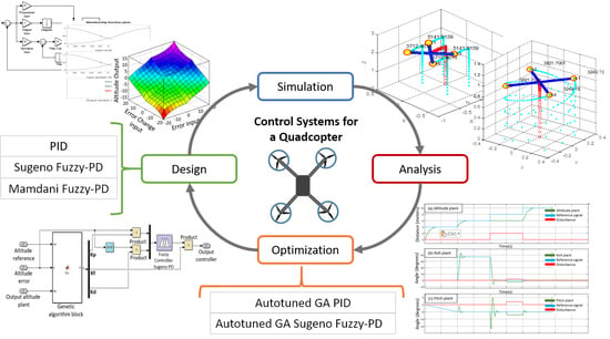


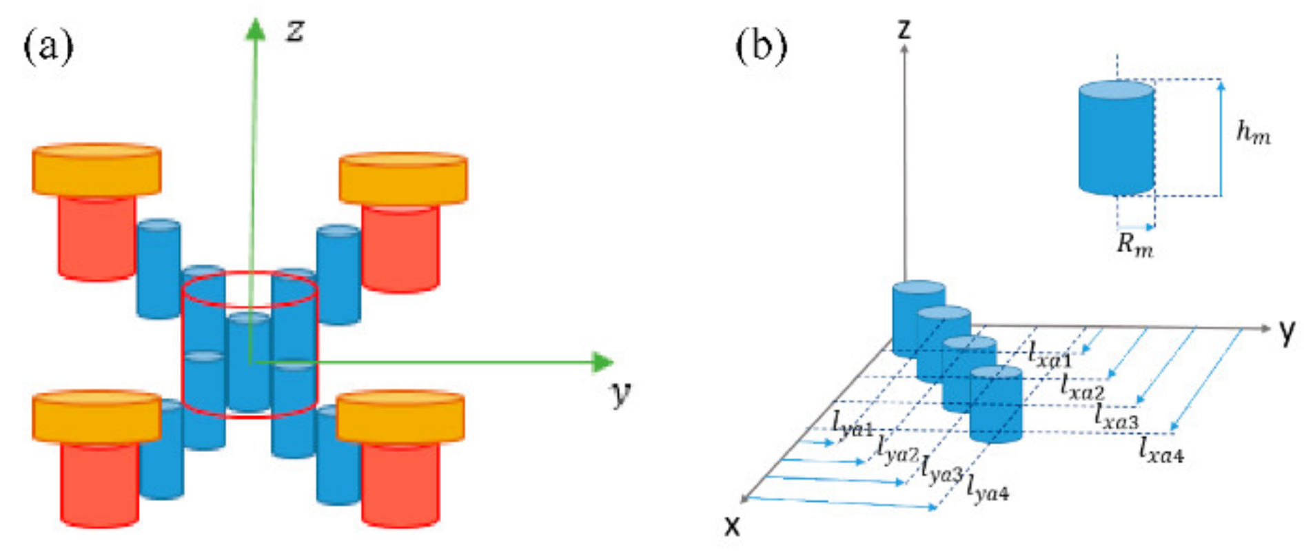
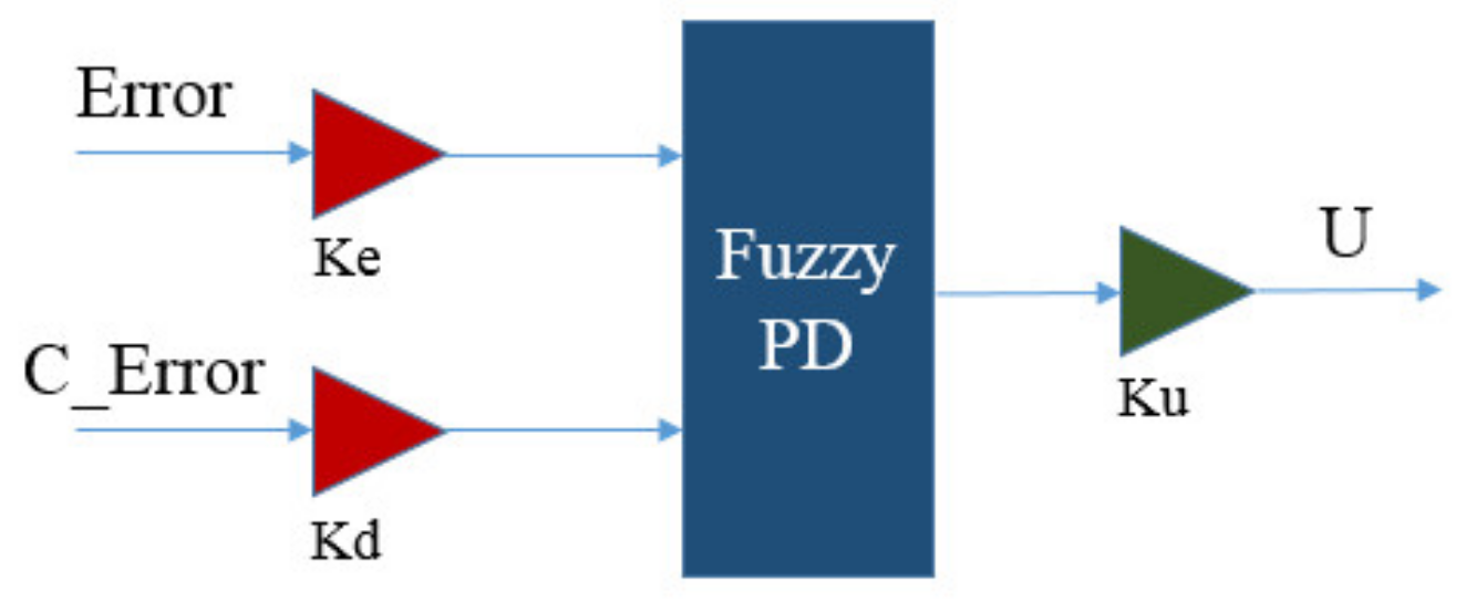
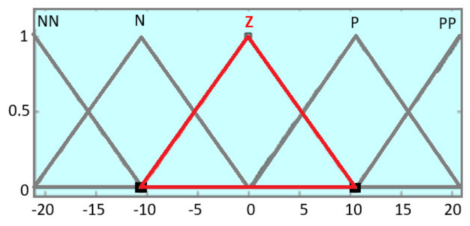
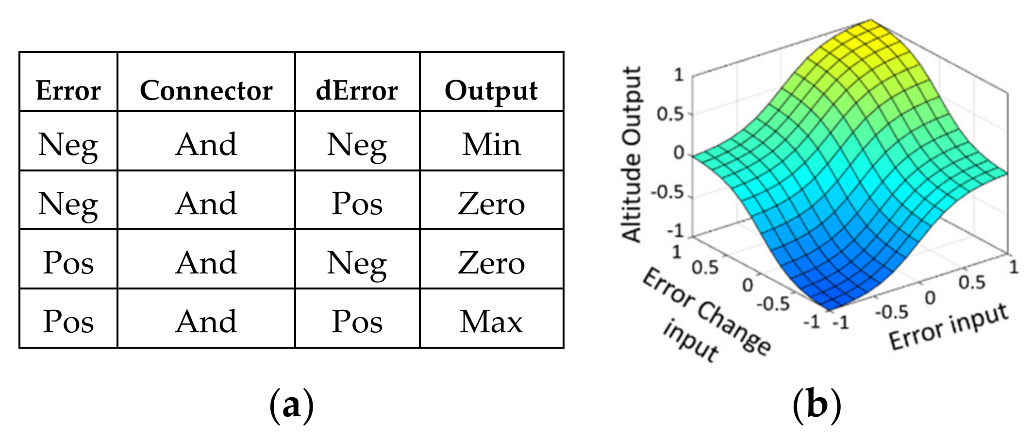
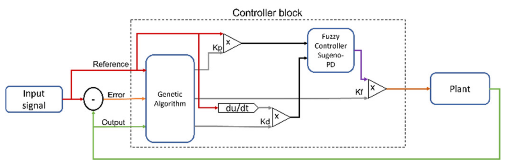
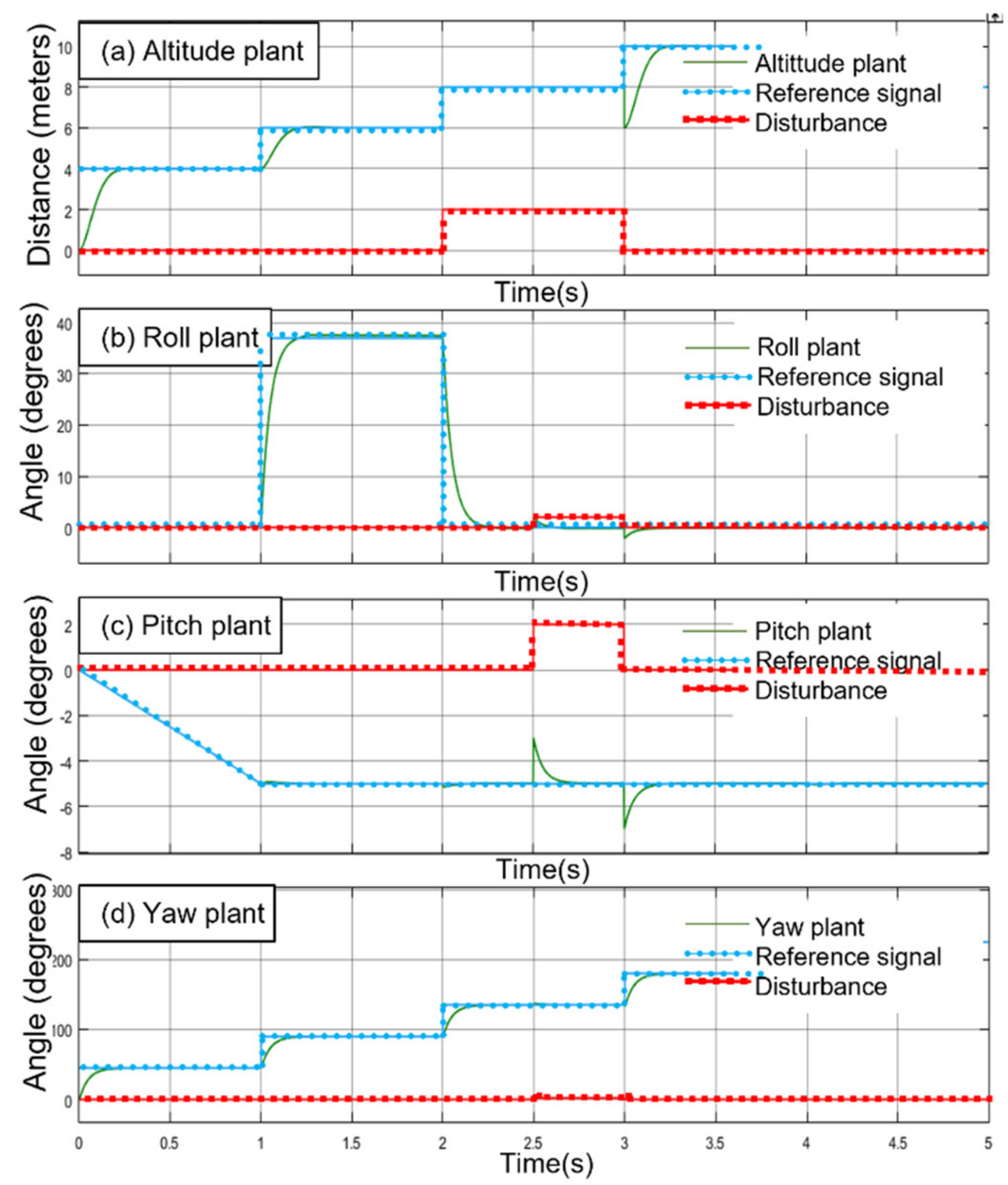