Article

Battery Durability and Reliability under Electric Utility Grid Operations: Analysis of On-Site Reference Tests

Hawaii Natural Energy Institute, School of Ocean and Earth Science and Technology, University of Hawai‘i Mānoa, Honolulu, HI 96822, USA
*
Author to whom correspondence should be addressed.
Electronics 2021, 10(13), 1593; https://doi.org/10.3390/electronics10131593
Submission received: 15 May 2021 / Revised: 29 June 2021 / Accepted: 30 June 2021 / Published: 2 July 2021

Abstract

:
Grid-tied energy storage will play a key role in the reduction of carbon emissions. Systems based on Li-ion batteries could be good candidates for the task, especially those using lithium titanate negative electrodes. In this work, we will present the study of seven years of usage of a lithium titanate-based battery energy storage system on an isolated island grid. We will show that, even after seven years, the modules’ capacity loss is below 10% and that overall the battery is still performing within specifications. From our results, we established a forecast based on the internal degradation mechanisms of the hottest and coldest modules to show that the battery full lifetime on the grid should easily exceed 15 years. We also identified some inaccuracies in the online capacity estimation methodology which complicates the monitoring of the system.

1. Introduction

Battery energy storage systems (BESS) play a key role in tomorrow’s grids as crucial building blocks towards higher integration of intermittent renewable energy generation [1,2,3,4,5]. This will be essential to allow small grids, such as the ones that power the Hawaiian Islands, to reach emission reduction targets. In Hawai‘i, the Renewable Portfolio Standards law mandates a 100% clean energy and transportation environment by 2045 [6].
Despite the large number of BESS deployed [7,8], most of the published studies so far are focused on modeling [9,10,11,12,13,14,15,16,17] with sizing, load modeling, or life cost analysis, as well as battery management system development [18,19]. Within the modeling studies, little to no effort was devoted to degradation modeling using realistic battery models.
In addition to the modeling studies, there are, to the best of our knowledge, only a few publications with results from field studies. Consiglio et al. [20] reported on the site acceptance test of a 0.5 MW system, Koller et al. [21] reported on the impact of different applications on a 1 MW system, Bila et al. [22] showcased initial performance of a grid connected household BESS. Some studies were more focused on field usage analysis. This includes our 3-year study of a grid deployed 1 MW BESS [23], a one year study for a 5 MW system by Münderlein et al. [24], the validation of smoothing algorithms [25], and some sweat testing under different applications [26]. In addition, the international Renewable Energy Agency reported results on some case studies [27,28]. Even Fewer studies reported electrochemical data. At the system level, Karouia et al. [29] compared Li-ion and a ZEBRA-based BESS of different sizes from 0.1 to 5 KW, and Kubiak et al. [30] analyzed the calendar aging induced degradation on a 250 kW/500 kWh system. At the cell level, and in addition to our previous work [31,32,33], Benato et al. [34] tested cells of different chemistries under realistic conditions, and Li et al. [35] tested nickel cobalt manganese cells for stationary applications. Finally, Podias et al., White et al., Elliot et al. as well as Zhang et al. investigated grid usage of recycled EV or bus batteries [36,37,38,39].
The Hawai‘i Natural Energy Institute (HNEI) at the University of Hawai‘i at Mānoa has been working on assessing the benefits of grid-scale BESS for the past decade [23,31,32,33,40,41,42]. One of our demonstration BESS is installed on the Hawaii Electric Light Company power grid on northern tip of the Big Island of Hawai‘i (star on the left of Figure 1) at the point of common coupling (PCC) between the 10.6 MW Hawaii Renewable Development Windfarm and the Waimea substation. It has been operational since December 2012 and consists of 384 modules in series with each module containing 7 cells in parallel. This amounts to a total of 268,850 Ah Altairnano Generation 1 cells composed of a lithium titanate (LTO) negative electrode (NE) and a blended positive electrode (PE) made of lithium cobalt oxide (LCO) and lithium nickel-cobalt-aluminum oxide (NCA) in a 55/45 ratio [32]. The modules are arranged symmetrically on both side of the container, Figure 1 right. The system is rated for 1 MW of power and 250 kWh of energy. The module nominal power is around 800 W which leads to a nominal power (P) for the BESS of 310 kW. Data, such as grid frequency and voltage, are logged by a Schweitzer SEL-735 meter at a 5 Hz sampling rate. Other data, such as cell group voltages and temperatures are sampled at 1 Hz. More details on the BESS and its installation can be found in [40]. HNEI’s work encompassed grid performance assessment, closed-loop control algorithms optimization to maximize grid support, as well as single cell and module laboratory testing for better understanding of degradation mechanisms. In previous works [23,31,32], three years’ worth of 1 MW/250 kWh Li-ion titanate BESS battery usage was analyzed and replicated on single cells leading to a forecast of cell durability based on the actual degradation observed in the laboratory.
In this work, the laboratory results will be compared with the real degradation associated with seven years of real usage on the grid where the BESS was primarily used for frequency regulation. This study will report on the durability of the BESS according to different metrics such as power, energy, efficiency, and capacity as calculated from two types of reference tests, one from the manufacturer and one custom. Moreover, a complete degradation analysis obtained from replaced modules will be used to discuss the accuracy of the online capacity estimation, the impact of modules temperature, the origin of the degradation, as well as to allow the forecast of the BESS remaining useful life using a realistic battery degradation model. The degradation model will be constructed from the evolution forecast for the three battery degradation modes: the loss of lithium inventory (LLI) and the loss of active material (LAM) on both electrodes [43].

2. Experimental

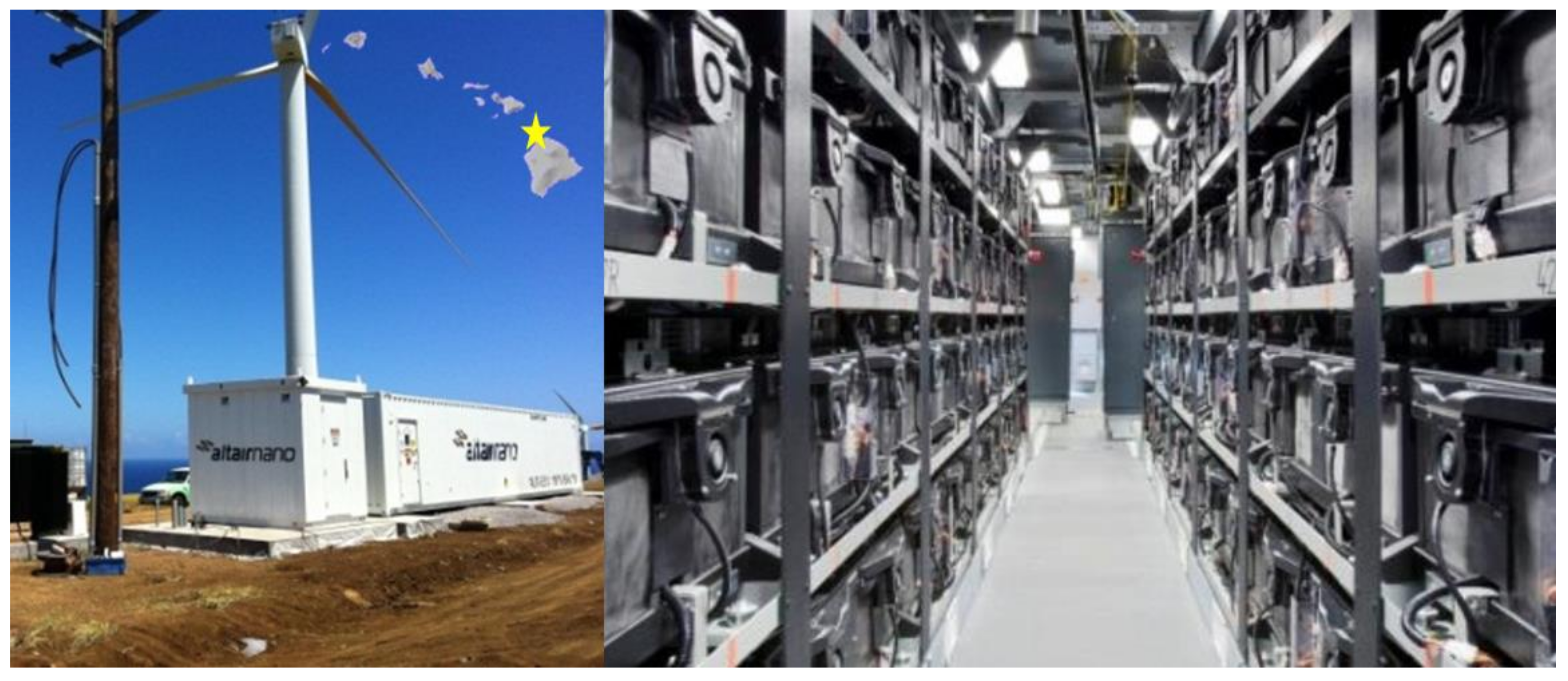
2.1. Overall Systems Description and Usage

The BESS stored close to 2.3 GWh of energy in seven years, which corresponds to 2.6 MAh of capacity or around 7500 equivalent full cycles. This represents more than 1000 equivalent full cycles a year or around 3 full cycles per day. Days of intense usage showcased more than 15 equivalent full cycles, black line on Figure 2. The system state of charge (SOC) was around 50% on average with daily excursions of 26% SOC. The average module temperatures were between 28 and 33 °C (with a 5 °C average temperature gradient within the modules). The overall usage of the BESS throughout its seven years of service is summarized in Figure 2. The hours of charging and discharging generally trended down starting in early 2015; this is due to adjustments to the primary frequency response algorithm that reduced cycling while still maintaining a significant portion of the grid benefit. This will be discussed in more detail in Section 4.1 below. A detailed analysis of the usage throughout the first three years was already published [23] and will not be repeated here. To assess the performance of the BESS, two types of periodic reference tests were performed, the manufacturer-recommended reference Test (MRT) and a custom HNEI reference test (HRT). The letters at the top of Figure 2 show when the tests were performed, with a blue M for the MRT and a red H for the HRT.

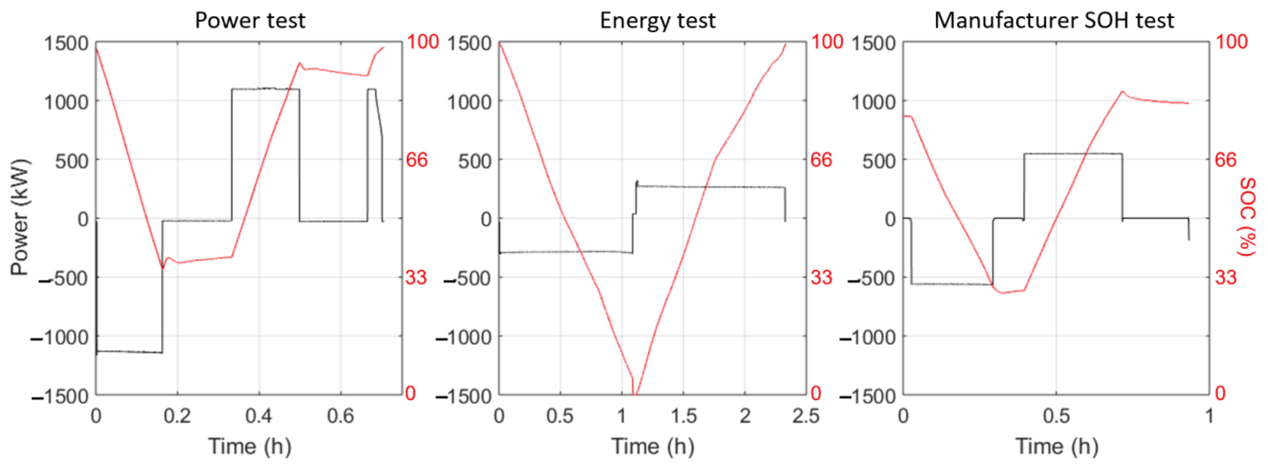
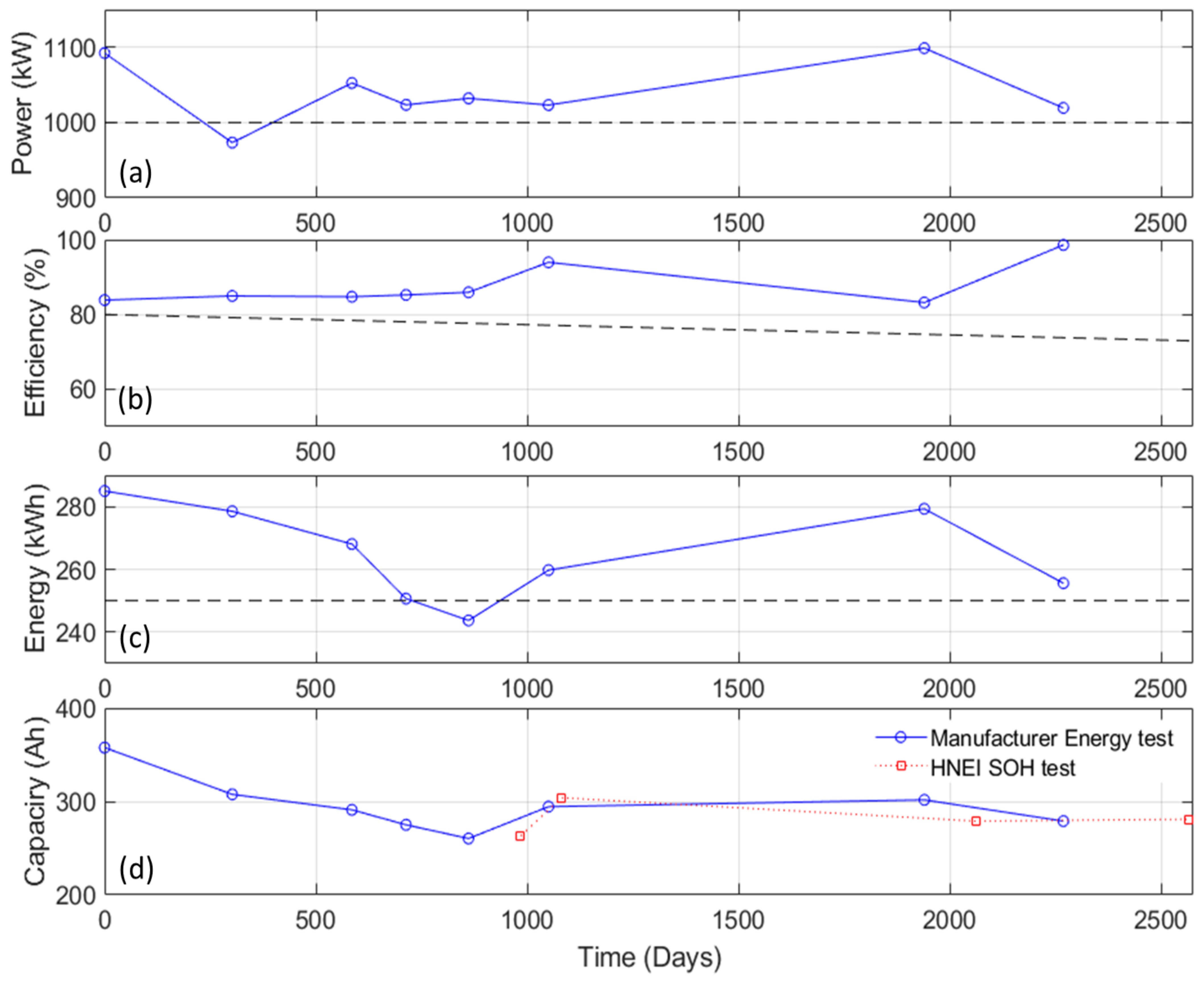
2.2. Manufacturer’s Reference Testing

The MRT consisted of three separate protocols to assess power ability, efficiency, energy ability as well as module capacities and resistances. The date at which those tests were carried on are highlighted by the letter M on the top of Figure 2. To date, the tests were repeated eight times at days 0, 302, 585, 713, 861, 1050, 1939 and 2268.
The power test consisted of 10 min 1 MW (3P) pulses in between 10 min rest periods. The test started and ended at a full charge state with the aid of a top-up pulse as shown in Figure 3. The first objective of this test is to first verify that the BESS can still provide over 1 MW of power at the PCC level. The second is to assess the power capability at the BESS level (i.e., how much power is needed to get 1 MW at the PCC level). The third is to calculate the efficiency (power in/power out).
To pass the test, the power rating must be above 1 MW and the efficiency rating above 80% minus 1% per year of service. The equations provided were the following:
P o w e r   r a t i n g = E d i s + E c h a 2 × 600   s × 3600   1.0   MW
E f f i c i e n c y   r a t i n g = E d i s + E r e s t _ d i s E c h a + E r e s t 2 + E r e s i d u a l   80 % 1 % / y e a r
The energy test consisted of a discharge and a charge at 250 kW (at PCC level, P/1.25) on the entire SOC range (0–100% from BESS SOC meter, denoted SOCB) with no rest in between as shown in Figure 2. The energy rating is calculated as the average of the charge and discharge energy. To pass the test, the energy storage capacity must be above 250 kWh. The equation provided by Altairnano was the following:
E n e r g y   S t o r a g e   c a p a c i t y = E d i s + E c h a 2   250   kWh
The state of health (SOH) test consisted of a charge and discharge at 500 kW (1.6P) between 30% and 80% SOC with 10 min rest periods before, in-between and after (Figure 3). The methodology to extract the module capacity and the resistance from this data was not explicitly stated by Altairnano but was assumed to be the following: for the module capacity, the rest cell voltages (RCV) should correspond to the open circuit voltage (OCV). From this OCV and a reference OCV vs. state of charge (SOC) curve, the ΔSOC between the two rests can be calculated. Dividing the corresponding measured capacity by the ΔSOC yield module capacity. For the module resistance, it was assumed that the ohmic drop (ΔV) between the rest and the application of the charge and discharge current were used. Based on the ohmic drops and knowing the current and Ohm’s law, the resistance can be calculated as R = ΔV/ΔI = ΔV/(I − 0) where I is the requested current and the “0” is the OCV current. Unlike the power and energy tests, the SOH test was not run consistently, and the charge and discharge power varied between 300 kW (2nd and 3rd iterations), 500 kW (1st, 5th,7th, and 8th iterations) and 1 MW (4th and 6th iterations).

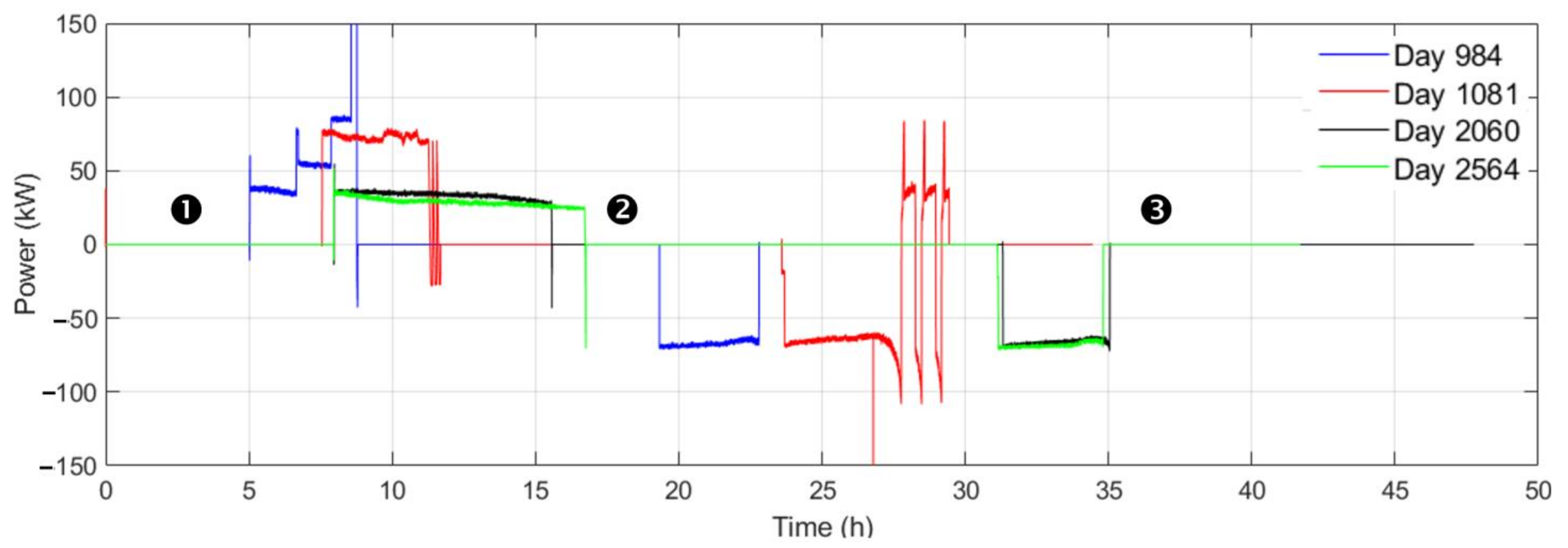
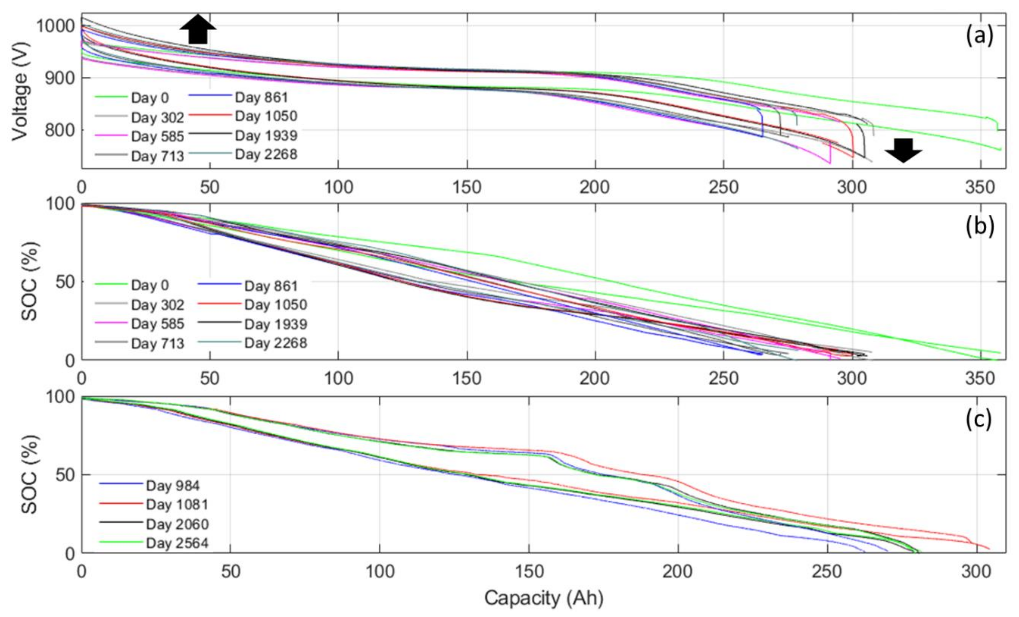
2.3. HNEI’s Reference Testing (HRT)

HNEI’s reference testing consisted of slow charge and discharge (50 kW, P/6.5) on the entire SOC window with long rests (>5 h vs. 10 min for MRT SOH test), Figure 4. This test was designed to accurately track capacity fading as well as changes in the modules OCV response. It also allowed the application of electrochemical voltage spectroscopies [44] such as incremental capacity (IC) to compare the degradation in the field to those observed in the laboratory [31,32]. Module capacities were extracted by dividing the measured capacity between two rests by the ΔSOC. This test could not be run often because it required significant downtime for the BESS (>40 h), but it was performed four times at days 984, 1081, 2060 and 2564. It also must be noted that there were some issues in the execution of the protocol for the first two iterations. In the first one, the charge power was not kept constant. In the second iteration, some pulses were performed at the end of the discharge prior to resting. Because of the significant downtime, tests could not be repeated and will therefore be analyzed as is.

2.4. HNEI’s Laboratory Battery Testing & Incremental Capacity Analysis

On two occasions, around day 1000 and 2500, some modules were replaced in the deployed BESS. The 12 removed modules were shipped to HNEI laboratory and tested on a calibrated 20-channel ARBIN LBT-25 V-100 A machine. Prior to the testing, all channels were current- and voltage-calibrated against a common reference (NIST-traceable Keithley 2700 source meter unit) to ensure consistency across the experiment. A reference performance test was performed at 25 °C and comprised C/25, C/10 and C/5 full cycles with 4-h rests before and after residual capacity measurements at C/50. More details on the reference test can be found in [45].
IC curve simulations were performed using the proprietary ‘alawa toolbox [46] using HNEI mechanistic degradation model [47]. Experimental validation supporting the simulation results based on LLI and LAM degradation modes has been reported by other groups [48,49,50]. The stock library of the ‘alawa toolbox was used for the half-cell data. More details on the process for these cells it out of the scope of this paper and it can be found in our previous work [32].

3. Results

3.1. Field Data

Figure 5a–c present the evolution of the power, efficiency, and energy ratings as a function of time. The power rating was stable for the seven years the BESS had been in service. It dropped slightly below 1 MW around Day 300 but recovered after. The efficiency also stayed above the threshold value throughout the 7 years of usage. The energy rating started above 280 kWh and quickly faded to around 240 kWh after day 800. This triggered the replacement of two modules around Day 1000. After modules replacement, the energy rating increased to around 270 kWh and remained rather constant between days 1000 and 2000 before starting to lower again.
Since both the MRT energy rating test and HNEI’s protocol were performed on the full SOC window, their exchanged capacity can be compared (Figure 5d). The BESS started with a capacity above 350 Ah which was expected with modules comprising 7 × 50 Ah cells in parallel. The capacity decreased to 260 Ah (−25%) before modules replacement and increased back to around 300 Ah (−15%) after then remained rather stable.
Figure 5c is intriguing as the available energy seems to increase between day 1000 and day 2000 from the MRT results. To investigate the origin of this increase, Figure 6a plots the voltage vs. capacity curves associated with all the MRT energy tests. From these plots, it is apparent that the overall end of discharge and end of charge potential are respectively increasing and decreasing (arrows on Figure 6a). This suggests that more of the voltage window of the cells is utilized and that therefore the ΔSOC used for the energy test is increasing. However, looking at the ΔSOCB (the SOC reported by the BESS), Figure 6b, it is always between 100 and 0. This indicates that SOCB does not have a 1:1 correspondence with the true SOC of the BESS. This is confirmed by the fact that SOCB and the capacity do not have a linear relationship, whether from the MRT test (Figure 6b) or the HRT test at low rate (Figure 6c). A deviation from a linear relationship can be seen at high and low SOC but also in the 40 to 60% region with a significant hysteresis especially visible in charge.
One of the most important features of the manufacturer’s and the HNEI’s SOH tests is the ability to estimate the capacity associated with each module. Because the modules are connected in series, they all see the same current and thus discharge the same amount of capacity. Therefore, the modules capacity cannot be deciphered directly. To calculate each module’s individual capacity, the exchanged capacity needs to be related with the associated ΔSOC in each module. This is usually done by using rest cell voltages and an OCV vs. SOC curve but this step is not straight forward, and multiple sources of error can arise. The first error source is usually caused by the fact the RCVs are not fully stabilized. Figure 7 presents an example of voltage vs. time curves for the six different RCVs considered in this work. Three RCVs were measured from the manufacture’s SOH test (①–③, Figure 3) that in most cases lasted less than 0.2 h and, the other three RCVs were measured from HNEI’s test (❶–❸, Figure 4) that lasted 5 h or more. Although all RCVs, even the short 10 min ones, appeared to be stable when the step was completed, the changes of voltages in the last 2 min of the relaxation steps were investigated to quantify the stability of the voltages. It was found that for RCVs ①–③, the potential still varied between 0.8 and 1.9 mV in average. For the long rests, the same measurement showed changes below 0.1 mV in average during the last 2 min. To address the significance of these changes, the voltage variations between 8 and 10 min of the long HRT relaxations were reviewed. They were found to be of 0.4 mV in average for ❶ and ❷ and around 5 mV for ❸. Moreover, the recorded potentials after 10 min were 5, 19 and 70 mV off the final voltage in average for ❶, ❷, and ❸ respectively. This shows that, although potentials ①–③ appear mostly stable after 10 min, they could be far from the OCV value since 0.4 mV variations after 10 min, lower that the one observed, could lead up to 70 mV further variation after several hours. The impact of these results, as well as other errors, will be discussed further in the next section.
Temperature is one of the most significant parameters to influence capacity retention and capacity loss. Figure 8 presents the evolution of the maximum daily maximum temperature as a function of day. The BESS was used more aggressively during the first 1000 days causing the temperature to be higher than for the latter days. Temperature stayed mostly below 40 °C. Also plotted in Figure 8 is the minimum module temperature at the same time as when the maximum was recorded. This showcases a temperature imbalance that could be responsible for some inhomogeneous degradation within the modules. The temperature difference between modules is typically between 5 and 10 °C.

3.2. Laboratory Data

The modules that were replaced were analyzed in HNEI’s battery testing laboratory. The modules in this BESS are organized in line replacement units (LRU) that each contain two modules. Therefore, with two LRUs replaced after 1000 days, four modules were exchanged. Of those, two were believed to be damaged (modules 25 and 170) and two behaved normally (modules 26 and 169). Four LRUs were also replaced after day 2500 including two that experienced the highest temperatures (modules 353 to 356) and two than experience the lowest temperatures (modules 201 to 204).
Figure 9a presents the C/25 discharge curves for the modules replaced at Day 1000 showing that only one the modules (#170) was actually defective with a capacity 15% lower than the others which were all within 1% around 384 Ah, close to the maximum capacity of 392 Ah from a pristine module [31]. For the modules changed after 2500 days, their capacities were between 387 and 393 Ah for the low temperature modules and between 386 and 389 Ah for the high temperature modules (Figure 9b).
To enhance the changes in the voltage response, Figure 9c,d display the modules’ incremental capacity (IC, dQ/dV = f(V)) signatures where it can be seen that they exhibited some differences in peak intensities which indicates disparities in SOH. Compared to a pristine cell, for which details can be found in [32], Feature A is broadened, Peak B is thinner, Peak D shrank and Peak E developed. All are clearly indicating (at least) loss of active material on both the positive and negative electrodes. Module 170 presents lower intensities for peaks B, C, D, and E compared to the other cells. Interestingly, the multiplication of the IC signature of module 170 by 7/6, nearly overlaps the signature of the other modules (dash curve). This indicates that the observed degradation might not be associated to an accelerated degradation but rather to the failure or disconnection of one of the cells in parallel within the module. The other module marked as defective (#25) did not show any specific difference compared to the others, which might indicate that there was an intermittent connection problem of one cell within the module. The single cells are encapsulated in a significant amount of hard resin, and they unfortunately could not be separated for individual testing despite some attempts. After 2500 days, the capacity differences between modules that experienced the same temperatures was minimal. Comparing modules that experienced higher temperatures to the lower temperature ones, Peak E is less intense and Peak A broader for the cells that were used at higher temperature. This suggests only a slight path dependence in the degradation process.

4. Discussion

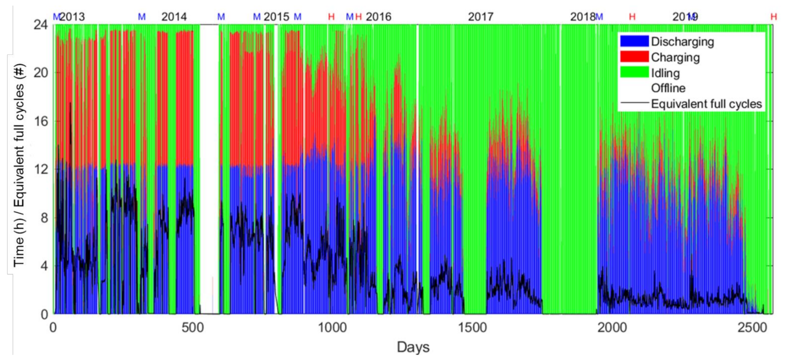
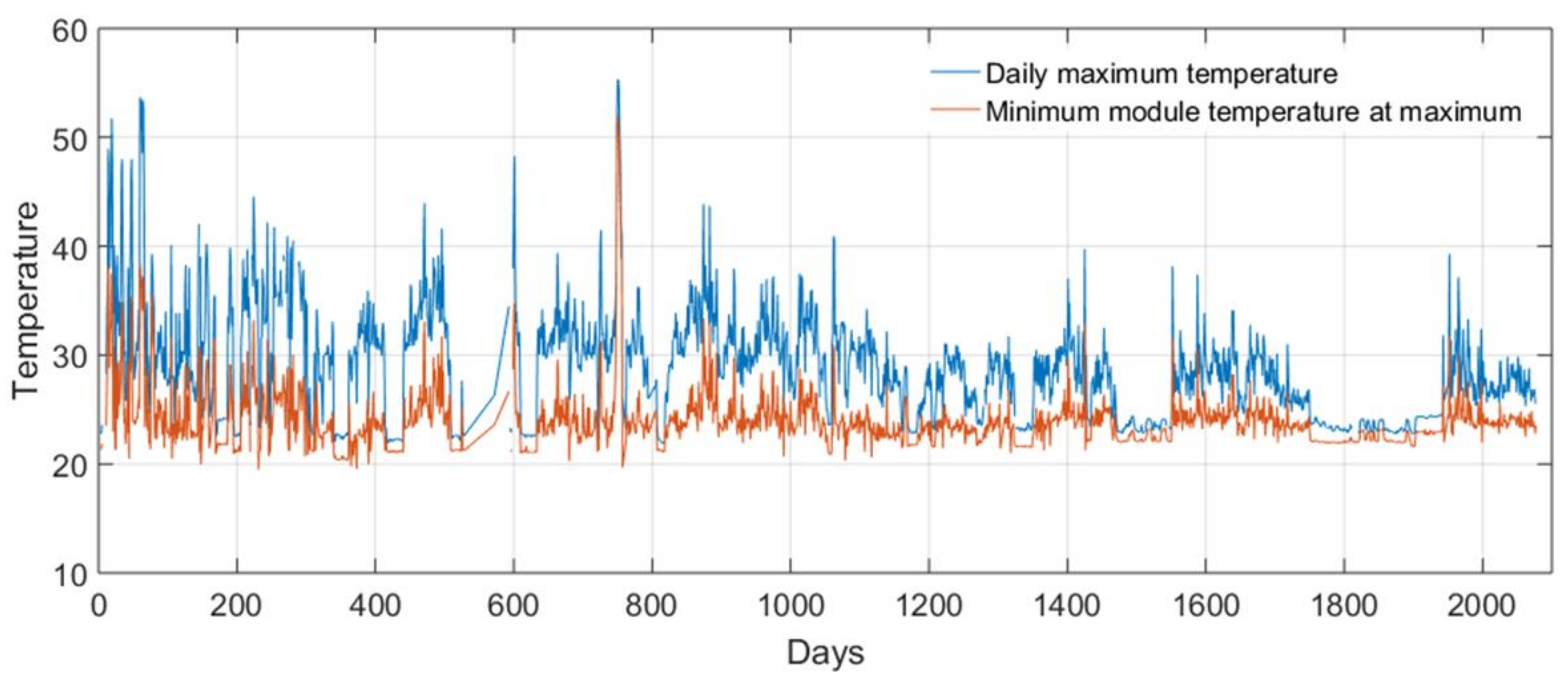
4.1. Overall Usage of the BESS

As showcased by Figure 2, the usage of the BESS varied throughout the 7 years of deployment. The BESS, installed at a 10.6 MW wind farm, is equipped with two real-time control algorithms: primary frequency response, and wind smoothing. The wind smoothing algorithm was rarely used (123 total days between 1 January 2013 and 31 December 2018). Between 2013 and 2014, the frequency response algorithm was generally fixed to an aggressive gain setting of 30 MW/Hz with no dead-band (a range of grid frequency deviations that are ignored by the BESS). Starting on 22 January 2015, dead-bands of 20 mHz and 40 mHz were tested along with gains of 20 MW/Hz, 30 MW/Hz and 40 MW/Hz. The BESS was also limited to respond with ±300 kW, ±500 kW, and ±1000 kW (max). Various combinations of settings were cycled over several days through June 2016 when the gain was set to 40 MW/Hz with a dead-band of 40 mHz for the remainder of the period. Further discussion on the impact of different settings in out of the scope of this paper and will be published at a later date.

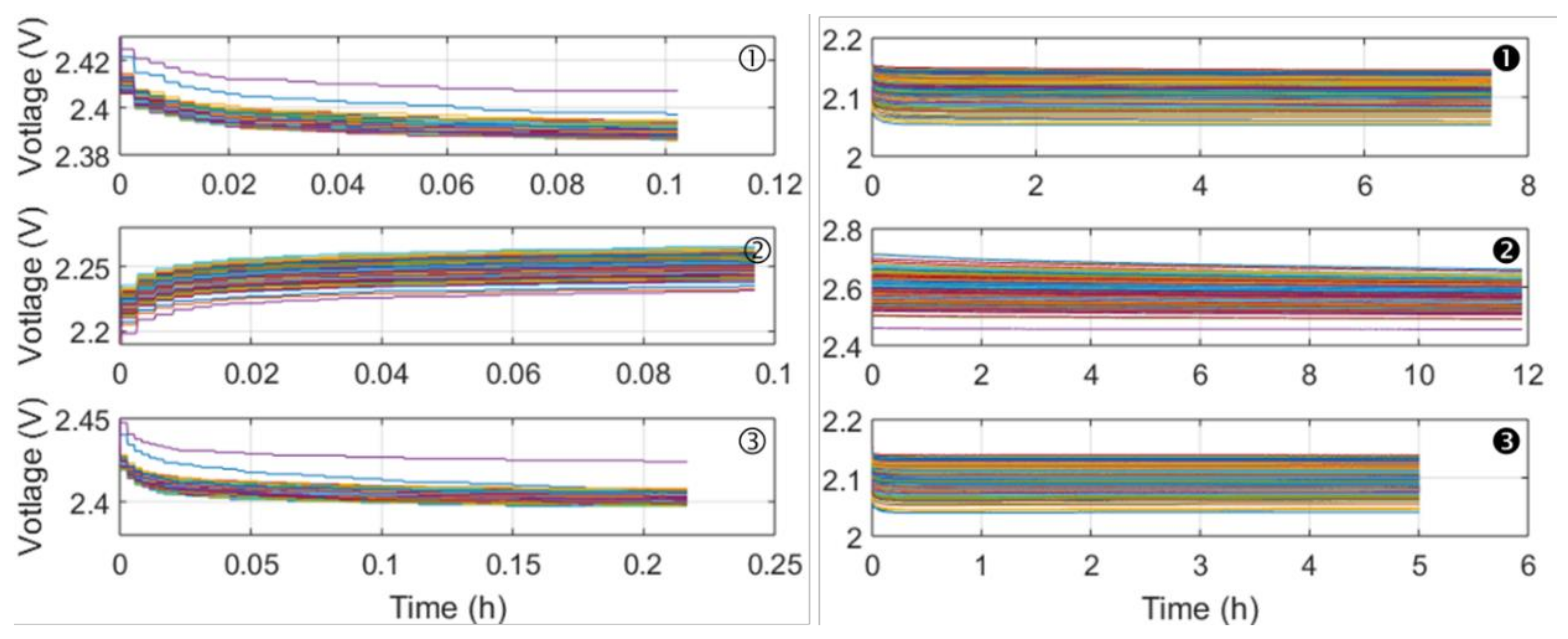
4.2. Open Circuit Voltages & Module Capacities

Proper indirect estimation of capacity requires satisfaction of several conditions:
-
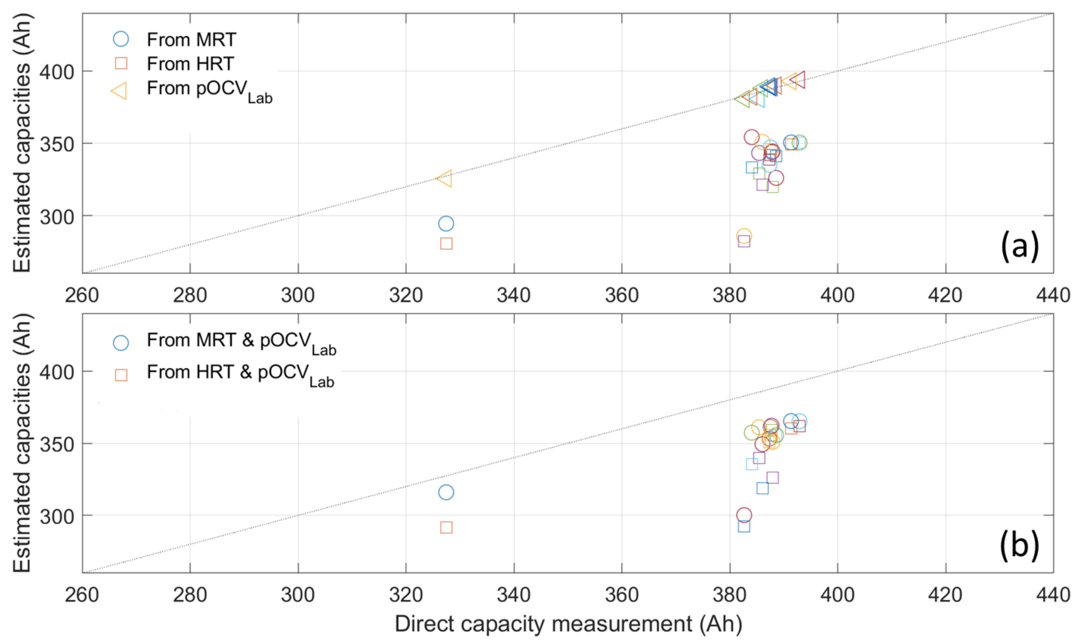
First, two good RCVs where the modules reached their equilibrium voltages. This usually requires long rests, ideally at a charged and discharged state.
-
Second, the measured RCVs must not be on a voltage plateau.
-
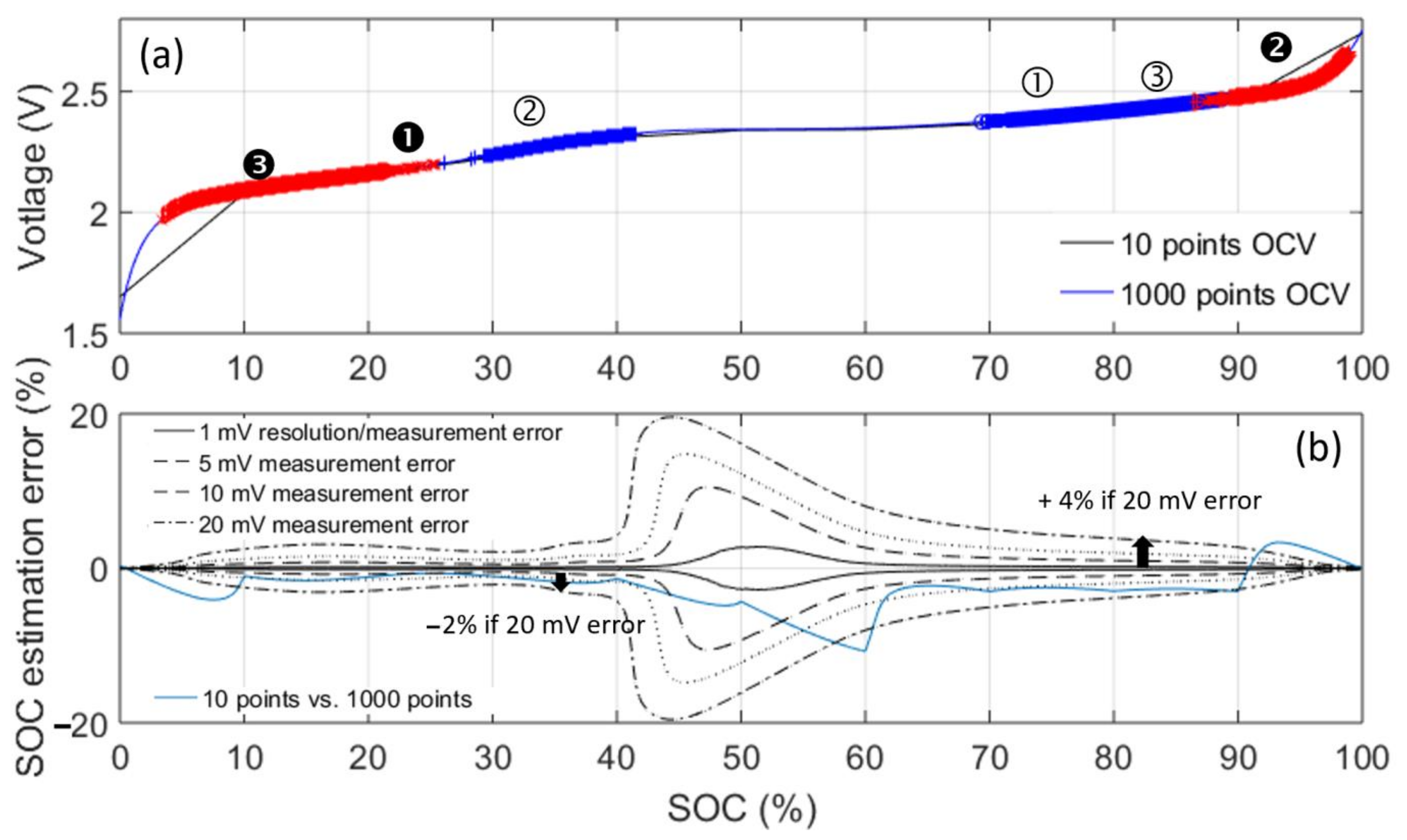
Third, an accurate OCV vs. SOC curve. Based on the information provided to us, Altairnano might be using a 10 points OCV vs. SOC curve. The method of interpolation between the points was not disclosed. From our laboratory testing, a higher resolution OCV vs. curve (1001 points, extracted from [31]) was available and used in this work.
-
Finally, the OCV vs. SOC curve needs to be updated upon aging. Depending on the battery degradation, the OCV vs. SOC curve will change with SOH as the cells degrade differently along with usage [32,43].
Figure 10b presents a comparison of a 10 and 1001 points OCV vs. SOC curve as well as associated SOC estimation errors. The error is around 3% on average with a maximum of 10% at 60% SOC. Figure 10b also provides the SOC estimation error based on RCV measurement errors of 1 mV (the resolution of the voltage sensors), 5 mV, 10 mV and 20 mV. According to our analysis of the relaxation curves (Figure 7) RCVs ①–③ were not stabilized and this could lead to significant errors since, for a 20 mV measurement error, SOC estimation could be on average ±5% off and up to ±20% off in the worst case scenario. The 1 mV resolution was found only be an issue only in the 45 to 55% SOC range were errors of ±2.5% are possible.
To start to quantify the possible errors on the capacity estimation, Figure 10a displays the spreads of RCVs for ①–③ and ❶–❸ on the initial OCV vs. SOC curve. None of them appear to be on a voltage plateau nor in areas of high possible SOC estimation errors. Nonetheless, the error induced by errors in voltage measurements up to 20 mV for ① and ③ could lead to SOC estimation errors up to 4% and 2% for ②. This SOC estimation error leads to ΔSOC errors in the order of 5% between the low and high SOC points and thus up to 10% underestimation of the capacity (5% on a ~50% SOC range), which is significant.
It must be noted that the shape of the error is similar to the observed mismatch between SOC and normalized capacity (Figure 6). Discussion on the evolution of the OCV curves with aging will be provided in the next section.
With three sets of relaxation voltages available per dataset, module capacities could be calculated between points 1 and 2 as well as between points 2 and 3. Figure 11a presents the comparison between the two sets of capacities estimated from rests ①–② and from rests ②–③. If the SOC determination was accurate, they should be equal. They are close except for the test at Day 713 where capacities calculated from points ①–② are 40 Ah higher (~10%) than the one measured from points ②–③. From a closer look at the data, the rests all look ok, but the charge capacity between ② and ③ was abnormally high. The origin of that capacity measurement error is unclear but likely associated with a calibration error for the current or the coulomb counting in charge. For the HRT test, Figure 11b and rests ❶–❸, the calculated capacities are overlapping for the first and fourth tests. For the second and third tests, there is an almost constant difference of 20 Ah and 10 Ah respectively. The origin of this difference is also likely related to calibration differences. Since the last four MRT tests were performed at similar time as the HRT tests, the calculated capacities can be compared and Figure 11c showcases the comparison of capacities ①–② and ❷–❸ for the four common tests, all gathered during the same regime and thus the same calibration. MRT capacities were all overestimated for Test 1, underestimated for tests 2 and 3 and scattered for Test 4. This illustrates that the correlation between the two datasets was weak at first then fast decreasing (Pearson correlation coefficient of 0.75, 0.4, 0.4 and 0.03 respectively for days 984, 1081, 2060, and 2564). This is interesting because it shows that the voltage measurement error impact is different for every module as the error is not constant. The accuracy of the MRT-determined capacities could potentially be improved by extrapolating the relaxation curves to estimate the final voltages [51,52] but this is out of the scope of this work. Figure 11 also shows that the module changes at Day 1000 did perturb the system significantly as the correlation coefficient dropped from 0.75 to 0.4 in less than 100 days. Finally, on both the HRT and the MRT test prior to Day 1000, two modules are consistently showing capacities around 30 Ah lower than the spread of others. These were the replaced modules.
Figure 12 presents the measured capacity loss versus time for both the MRT and the HRT experiments. Since no initial point was available for the HRT experiment, the maximum capacity measured during our cell-to-cell variation analysis [31], with the calendar aging accounted for, was used as a starting point. It seems that the modules did not degrade homogenously as the difference in capacity loss in-between modules spans for more than 15% after 2500 days with between 10 and 25% capacity loss (HRT test). According to the MRT results, this spreading might have been gradual. The inaccuracy of the MRT is exemplified by the capacity loss going up and down depending on the test. It must be noted that the capacity loss on the modules did also decreased for the HRT test after module replacement. The origin of this is unclear at this point but it might be associated to the BESS being set offline for while awaiting module replacement as capacity can sometimes be recovered after long rests. This might be related to a change in calibration or with electrode overhang and the fact that some lithium ions that migrated to the inactive part of the electrode can migrate back into the active area [53]. Some of the new modules also appear to degrade faster than the rest of the modules which resembles the fast capacity loss observed during the first 300 days for the other modules.
The increase of the spread of capacity loss between modules can usually be attributed to different usage patterns, different temperatures and different intrinsic degradation rates [54]. All modules are in series, so they all experience the same current. Since modules are comprised of seven cells in parallel, it is possible that some cells were used more than others within the modules. However, our recent modeling work on the impact of cell-to-cell variations in modules with cells in parallel showed limited impact of inhomogeneous degradation on the module performance [55]. The second possible contributing factor is the temperature. Some temperature gradients were observed within the BESS (Figure 8) and it is therefore possible that the hottest modules degraded faster than the coolest ones. An analysis of the module temperatures showed that the same modules were consistently hotter than others. Figure 13a shows the positions of these modules within the BESS. Hotter modules were on the top row near the middle of the stack on both sides. Cooler modules were always on the bottom. Figure 13b compares the capacity losses with modules average temperatures and Figure 13c the capacity loss with the time each module spent above 35, 45 and 50 °C. In all cases, Pearson correlations coefficient are below 0.15, there is therefore no impact of the temperature on the modules’ inhomogeneous degradation. This was verified for both HRT and MRT measured capacities. This was also validated with direct capacity measurement from the replaced modules (Figure 9) that experienced the highest and lowest average temperatures and show less than 1% capacity difference in average. Another explanation for the spread of capacity loss could be the intrinsic degradation rate [54]. Previous studies on other types of cells showed differences of more than 5% after 1000 cycles, therefore 10% after 6500 cycles is not out of the range of possibilities. This is tempered however by the laboratory test results where the four replaced modules for each temperature (both at low and high) were compared and where the observed maximum spread between the cells was around 1%, higher than in between different temperatures, but much lower than 10%.
Based on the observations above, the most likely explanation could be inaccuracies in capacity estimation. Such inaccuracies can originate from inadequate rest cell voltage measurements, inaccurate OCV vs. SOC curves and errant capacity measurements. An easy way to determine if there is any significant error in the capacity estimation is to compare the last capacity estimated for the 12 modules that were replaced with the one directly measured during the laboratory tests, Figure 14. Figure 14a presents the comparison of the estimated capacity versus the measured capacity for the 12 modules that were replaced. The estimated capacities show neither precision nor accuracy. All were underestimated by at least 8% and by more than 13% in average and their correlation was also rather weak at 0.6 and 0.7 for the MRT and the HRT respectively. To verify the validity of the capacity estimation method, the capacity obtained during the laboratory test were also estimated using both the initial OCV curve and an updated OCV curve, calculated from averaging the C/25 charge and discharge [45], for each module (triangles in Figure 14a). In both cases, the estimated capacity is at most of 0.7% different than and the measured one with a correlation higher than 0.99. This illustrates that, for these cells and under these conditions, the accuracy of OCV curve used does not matter much if the cells rest in areas of limited error towards the end of charge and the end of discharge (Figure 10). This is confirmed by Figure 14b where the module capacities were estimated using the RCV measured from the MRT and HRT tests and the true OCV curve for each module (calculated from the HRT test). Figure 14b shows marginally better estimation with an average error of 9% (4% less) and the same correlation. The estimation difference is higher between the two OCV curves because, from the BESS, the measured relaxations were not truly at the end of charge and the end of discharge and thus in areas of larger error (Figure 10). The impact of the quality of the rest cell measurements has already been discussed and should not be a major factor for the HRT dataset, therefore this error must originate elsewhere.
With errors coming from the accuracy of the OCV curves and the one from RCV removed, the only possibility left is some inaccuracies in the capacity measurements. This was not considered at first because, since all the modules are in series, this error was believed to be constant. However, the different calibration issues observed Figure 11 seems to show that there might be some problems. This was acknowledged by the manufacturer and this could explain the accuracy issue. In addition, one important parameter was not considered: cell balancing. In the BESS, balancing is continuous throughout the SOC range whenever the lowest cell group SOC is greater than or equal to 5%. The lowest SOC cell group is compared to all other cell groups to determine balance of the BESS. Any cell group that is Δ3% SOC or more compared to the lowest cell group SOC will receive a 150 mA resistive load to remove energy from the cell group. Therefore, modules might receive more capacity than was recorded in our data, and this could explain the precision issues. Balancing data was unfortunately not available to us.

4.3. Degradation Analysis

Despite the setback in not being able to track the real capacity loss from all the modules, we can still investigate the degradation based on the modules that were removed from the BESS. In our previous work [32], the electrochemical behavior of the single cells was investigated and a sensibility analysis was performed to determine the most relevant features of interest (FOI) to diagnose the degradation mechanisms. Based on this analysis, the loss of active material on both component of the PE, LAMNCA and LAMLCO respectively and of the NE (LAMNE) were decipherable directly from FOIs. The last degradation mode, the loss of lithium inventory, had to be estimated from the best possible fit of the electrochemical behavior. The three FOI were the area between 2.3 and 2.4 V to quantify LAMLCO, the area between 2.15 and 2.3 V to quantify LAMNCA and the intensity at 2.44 V to quantify the total LAMPE. Given the shape of the IC curves, no capacity appears to be outside of the potential window and therefore, LAMNE was estimated from the capacity loss.
Based on the FOIs and the methodology we proposed in [32] to quantify the degradation mechanisms on these cells, the degradation of the lower temperatures modules comprised, on average, 5.2 (±2.6)% LAMLTO, 7.6 (±0.8)% LAMNCA, 1.9 (±0.8)% LAMLCO, and 6.0 (±0.9) LLI. For the higher temperature modules, the degradation was composed of 5.9 (±2.2)% LAMLTO, 13.5 (±3.2)% LAMNCA, 2.6 (±1.0)% LAMLCO, and 8.8 (±0.9) LLI. The observed ratios between the degradation modes are comparable to the one measured during the laboratory experiment [32]. This confirms that our laboratory test was successful in replicating realistic aging for the BESS system.
Since the data for the MRT energy and HRT tests were done on the entire SOCB range at a relatively low rate for high power cells, P/1.25 and P/6.5, the same FOI analysis was tried on the field data. Unfortunately, it was found not to be possible as the FOI values extracted from the tests before the modules swap did not match the one observed experimentally in the laboratory for the replaced modules. This could be related to several issues: First, the voltage response at the single level is rather noisy and so significant smoothing was necessary to have clear IC features which modify IC peaks shape, area and intensity and thus FOI detection. Second, the HRT and MRT tests were done under constant power regime which affected the IC peaks at beginning and end of regime where voltage variations are significant and where FOI 2 and 3 were measured. Third, not all the cells used the same SOC range and so, information was missing for some cells. Finally, as shown above, the capacity cannot be estimated with accuracy and thus LAMNE is not quantifiable directly which hampers the derivation of LLI even if the LAMPE was accurate. For interested readers, the obtained IC curves for the MRT test after smoothing are presented in Figure A1 in Appendix A. No sign of LAMPE induced capacity loss was found. LLI does not seems to be a factor in capacity loss either, but it is impossible to be sure because most cells did not reach their end of charge cutoff before 100% SOCB. From what is observable, it appears that none of the modules have started any accelerated degradation stage at the time of this writing.
One solution to estimate the remaining useful life for the deployed BESS is to extrapolate from the diagnosis that was performed on the replaced modules in the laboratory. If the observed degradation is considered normal, these trends can be extended and they should be representative. Our analysis showed an increasing spread in between cells and to take that into account, the extent of each degradation will be varied in the simulations to accommodate inhomogeneous aging pace. Simulations were performed from the average values for lower and higher temperature modules as well as with variations corresponding to one- and two-times the observed standard deviation, σ. All combinations of standard deviations (on the three LAMs and LLI) were simulated and only the worst-case scenario was plotted. Results from these simulations are presented in Figure 15. From the degradation mode quantification, and if the BESS usage remained consistent, an acceleration of the aging could start around day 2500 (~seven years) for the higher temperature modules only if the cell-to-cell variations are in the 2σ range and in the worst-case scenario (lower than average LLI and LAMLCO, higher than average LAMLTO and LAMNCA). If within σ, accelerated aging only stars after 14 years of usage under the same conditions. For the modules at lower temperatures, no significant acceleration is expected within 20 years of usage. Since our observations at Day 1939 (Figure A1) show no sign of accelerated aging, the BESS is believed to be in the middle to upper portion of the spread and thus be able to last up more than 15 years with capacity loss on the modules below 30%.

5. Conclusions

This study spans more than seven years of usage of a grid-tied BESS system on the Island of Hawai‘i in the Hawaiian archipelago. The BESS has been well used and is continuing to provide significant storage capability for the grid. Its performance is still within specifications and the only maintenance performed was the replacement of two modules that appeared to suffer from the disconnection of one of the seven cells in parallel. Despite some temperature inhomogeneities, with some modules running consistently 5 °C or more hotter than others, the capacity of the BESS was not affected much with a difference of around 1% between the hottest and the coolest modules. However, the temperature induced a slightly different degradation pattern that might induce accelerated degradation for the hotter modules later in life. The overall capacity loss on the modules was estimated to be between 5 and 10% after 7 years of usage compared to 15% at the BESS level. This calculation was only obtainable from swapped modules after 2500 days of usage. The internal module capacity estimation was vastly overestimated by between 10 and 25% despite our best efforts. We believe that inaccuracies in the capacity measurement, and the lack of information on the balancing, prevented the correct estimation. This could prove problematic for future deployments and better solutions need to be enacted to ensure accurate estimation. This could include better safeguards for capacity estimation and the option to stop balancing, or monitor it better, while performing reference tests. Nonetheless, the BESS is performing well and, according to the forecast, its useful lifespan should exceed 15 years on the grid with a capacity loss below 30%.

Author Contributions

Conceptualization, M.D.; data harvesting, M.T.; methodology, M.D.; formal analysis, M.D.; writing—original draft preparation, M.D. and M.T.; writing—review and editing, M.D., G.B., M.T., M.M. and R.E.R. All authors have read and agreed to the published version of the manuscript.

Funding

This work was supported by the State of Hawai‘i and ONR Asia Pacific Research Initiative for Sustainable Energy Systems (APRISES), award numbers N00014-17-1-2206, N00014-18-1-2127 and N00014-19-1-2159.

Acknowledgments

The authors also would like to thank Karl Stein, Marc Matsuura, Keith Musser, Keith Bethune, Jack Huizingh (HNEI) as well as Brad Hanauer and Michael Brunell (Altairnano) for their help through the course of this study.

Conflicts of Interest

The authors declare no conflict of interest. The founding sponsors had no role in the design of the study; in the collection, analyses, or interpretation of data; in the writing of the manuscript, and in the decision to publish the results.

Abbreviations and Nomenclature

The following abbreviations was used in this manuscript:
BESSBattery Energy Storage System
FOIFeature of Interest
HNEIHawaii Natural Energy Institute
HRTHNEI Reference Test
ICIncremental Capacity
LAMLoss of Active Material
LCOLithium Cobalt Oxide
LLILoss of Lithium Inventory
LRULine Replacement Unit
LTOLithium Titanium Oxide
MRTManufacturer Reference Test
NCANickel Aluminum Cobalt Oxide
NENegative Electrode
OCVOpen Circuit Voltage
PEPositive Electrode
PCCPoint of Common Coupling
RCVRest Cell Voltage
SOHState of Health
SOCState of Charge
The following nomenclature was used in this manuscript:
-
P/x refers to rated power usage, P/1 being a full charge or discharge in 1 h.
-
Black circled numbers refer to the RCV measured during the HRT test.
-
White circled numbers refer to the RCV measured during the MRT test.
-
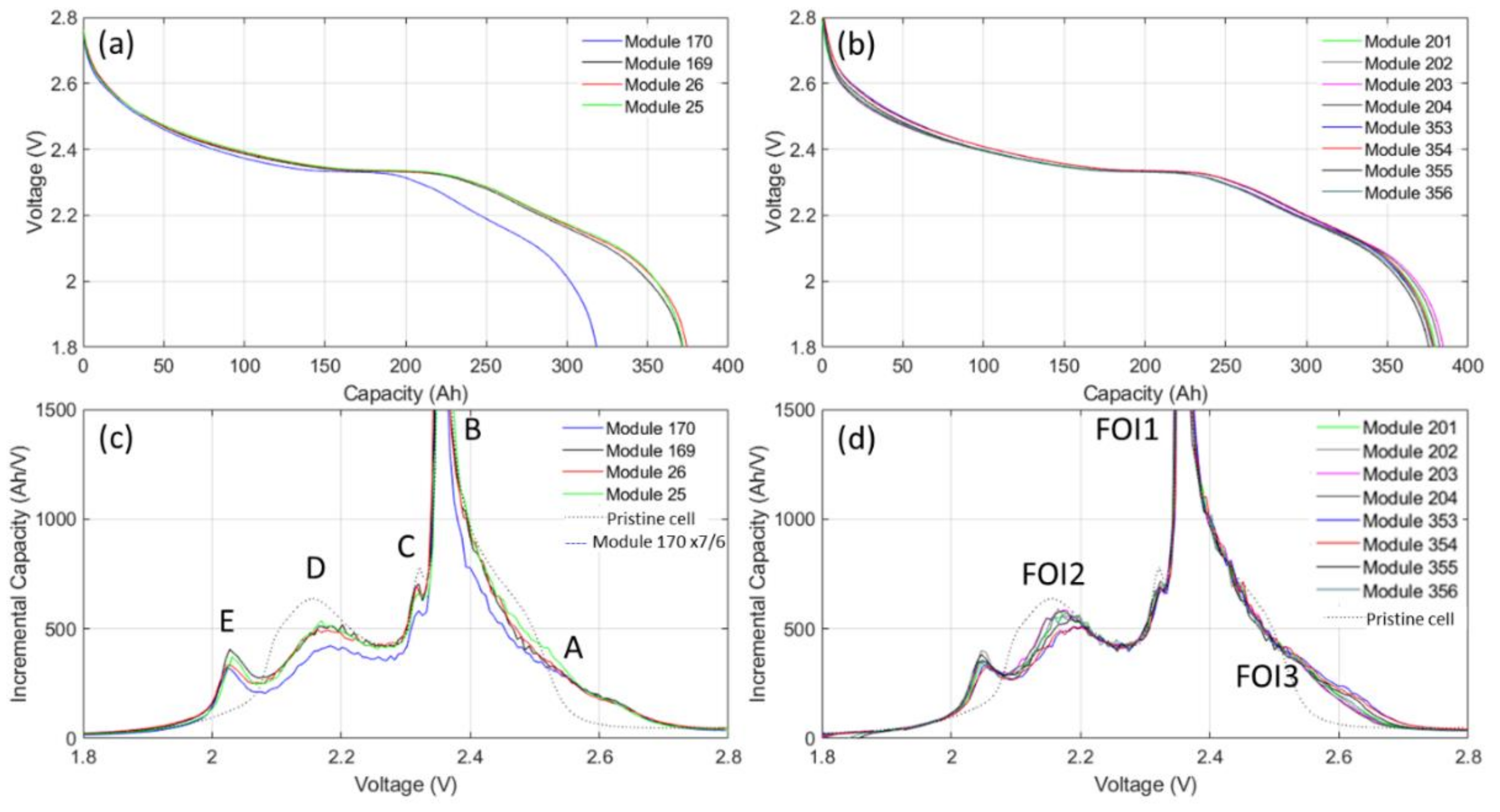
Letters A to F refer to electrochemical peaks on Figure 8.
-
Q refers to capacity, V to voltage, and I to current.

Appendix A

Figure A1 presents the IC curves (dQ/dV = f(V)) for the 384 modules gathered from the MRT test at days 0, 302, 585, 713, 861, 1050, and 1939. The voltage curves were smoothed before derivation. The modules electrochemical behavior is homogeneous in the early days then some imbalance starts to be visible from day 585. Because of the growing imbalance, the lowest voltage peak and the high voltage shoulder starts to be inaccessible for some cells which affected the overall BESS capacity retention. This explain why the capacity loss of the BESS seems to be higher than the one of the modules. At day 1939, the voltage response of the modules shows no sign of accelerated aging.
Figure A1. IC signatures for the charges during the energy test. Different colors correspond to the BESS 384 modules.
Electronics 10 01593 g0a1

References

  1. Yang, Y.; Bremner, S.; Menictas, C.; Kay, M. Battery energy storage system size determination in renewable energy systems: A review. Renew. Sustain. Energy Rev. 2018, 91, 109–125. [Google Scholar] [CrossRef]
  2. Mohamad, F.; Teh, J. Impacts of Energy Storage System on Power System Reliability: A Systematic Review. Energies 2018, 11, 1749. [Google Scholar] [CrossRef] [Green Version]
  3. Stecca, M.; Ramirez Elizondo, L.; Batista Soeiro, T.; Bauer, P.; Palensky, P. A Comprehensive Review of the Integration of Battery Energy Storage Systems into Distribution Networks. IEEE Open J. Ind. Electron. Soc. 2020, 1. [Google Scholar] [CrossRef]
  4. Datta, U.; Kalam, A.; Shi, J. A review of key functionalities of battery energy storage system in renewable energy integrated power systems. Energy Storage 2021. [Google Scholar] [CrossRef]
  5. Elshurafa, A.M. The value of storage in electricity generation: A qualitative and quantitative review. J. Energy Storage 2020, 32. [Google Scholar] [CrossRef]
  6. Lee, T.; Glick, M.B.; Lee, J.-H. Island energy transition: Assessing Hawaii’s multi-level, policy-driven approach. Renew. Sustain. Energy Rev. 2020, 118, 109500. [Google Scholar] [CrossRef]
  7. Subburaj, A.S.; Pushpakaran, B.N.; Bayne, S.B. Overview of grid connected renewable energy based battery projects in USA. Renew. Sustain. Energy Rev. 2015, 45, 219–234. [Google Scholar] [CrossRef]
  8. Department of Enegy. DOE Global Energy Storage Database. Available online: http://www.energystorageexchange.org/projects (accessed on 13 June 2021).
  9. Khasawneh, H.J.; Mondal, A.; Illindala, M.S.; Schenkman, B.; Borneo, D. Evaluation and Sizing of Energy Storage Systems for Microgrids. In Proceedings of the 2015 IEEE/IAS 51st Industrial & Commercial Power Systems Technical Conference (I&CPS), Clagary, AB, Canada, 6–8 May 2015. [Google Scholar]
  10. Shen, J.; Dusmez, S. Optimization of Sizing and Battery Cycle Life in Battery/Ultracapacitor Hybrid Energy Storage Systems for Electric Vehicle Applications. IEEE Trans. Ind. Inform. 2014, 30, 2112–2121. [Google Scholar] [CrossRef]
  11. Lu, C.; Xu, H.; Pan, X.; Song, J. Optimal Sizing and Control of Battery Energy Storage System for Peak Load Shaving. Energies 2014, 7, 8396–8410. [Google Scholar] [CrossRef] [Green Version]
  12. Liu, M.; Li, W.; Wang, C.; Polis, M.P.; Wang, Y.L.; Li, J. Reliability Evaluation of Large Scale Battery Energy Storage Systems. IEEE Trans. Smart Grid 2016, 1–11. [Google Scholar] [CrossRef]
  13. Zakeri, B.; Syri, S. Electrical energy storage systems: A comparative life cycle cost analysis. Renew. Sustain. Energy Rev. 2015, 42, 569–596. [Google Scholar] [CrossRef]
  14. Marini, A.; Latify, M.A.; Ghazizadeh, M.S.; Salemnia, A. Long-term chronological load modeling in power system studies with energy storage systems. Appl. Energy 2015, 156, 436–448. [Google Scholar] [CrossRef]
  15. Parlikar, A.; Hesse, H.; Jossen, A. Topology and Efficiency Analysis of Utility-Scale Battery Energy Storage Systems. In Proceedings of the 13th International Renewable Energy Storage Conference (IRES 2019), Dusseldorf, Germany, 12–14 March 2019. [Google Scholar]
  16. Reniers, J.M.; Mulder, G.; Howey, D.A. Unlocking extra value from grid batteries using advanced models. J. Power Sources 2021, 487. [Google Scholar] [CrossRef]
  17. Ren, D.; Lu, L.; Shen, P.; Feng, X.; Han, X.; Ouyang, M. Battery remaining discharge energy estimation based on prediction of future operating conditions. J. Energy Storage 2019, 25. [Google Scholar] [CrossRef]
  18. Gabbar, H.A.; Othman, A.M.; Abdussami, M.R. Review of Battery Management Systems (BMS) Development and Industrial Standards. Technologies 2021, 9, 28. [Google Scholar] [CrossRef]
  19. Lelie, M.; Braun, T.; Knips, M.; Nordmann, H.; Ringbeck, F.; Zappen, H.; Sauer, D. Battery Management System Hardware Concepts: An Overview. Appl. Sci. 2018, 8, 534. [Google Scholar] [CrossRef] [Green Version]
  20. Consiglio, L.; Di Lembo, G.; Noce, C.; Eckert, P.; Rasic, A.; Schuette, A. Performances of the first electric storage system of Enel Distribuzione. In Proceedings of the International Conference and Exhibition on Electricity Distribution (CIRED), Stockholm, Sweden, 10–13 June 2013; IEEE: Stockholm, Sweden, 2013; pp. 1–4. [Google Scholar]
  21. Koller, M.; Borsche, T.; Ulbig, A.; Andersson, G. Review of grid applications with the Zurich 1MW battery energy storage system. Electr. Power Syst. Res. 2015, 120, 128–135. [Google Scholar] [CrossRef]
  22. Bila, M.; Opathella, C.; Venkatesh, B. Grid connected performance of a household lithium-ion battery energy storage system. J. Energy Storage 2016, 6, 178–185. [Google Scholar] [CrossRef]
  23. Dubarry, M.; Devie, A.; Stein, K.; Tun, M.; Matsuura, M.; Rocheleau, R. Battery Energy Storage System battery durability and reliability under electric utility grid operations: Analysis of 3 years of real usage. J. Power Sources 2017, 338, 65–73. [Google Scholar] [CrossRef]
  24. Münderlein, J.; Steinhoff, M.; Zurmühlen, S.; Sauer, D.U. Analysis and evaluation of operations strategies based on a large scale 5 MW and 5 MWh battery storage system. J. Energy Storage 2019, 24, 100778. [Google Scholar] [CrossRef]
  25. Jannati, M.; Foroutan, E. Analysis of power allocation strategies in the smoothing of wind farm power fluctuations considering lifetime extension of BESS units. J. Clean. Prod. 2020, 266. [Google Scholar] [CrossRef]
  26. Abedi Varnosfaderani, M.; Strickland, D.; Ruse, M.; Brana Castillo, E. Sweat Testing Cycles of Batteries for Different Electrical Power Applications. IEEE Access 2019, 7, 132333–132342. [Google Scholar] [CrossRef]
  27. IRENA. Case Studies: Battery Storage; International Renewable Energy Agency: Abu Dhabi, United Arab Emirates, 2015; pp. 1–20. [Google Scholar]
  28. IRENA. Battery Storage for Renewables: Market Status and Technology Outlook; International Renewable Energy Agency: Abu Dhabi, United Arab Emirates, 2015; pp. 1–60. [Google Scholar]
  29. Karouia, F.; Ha, D.-L.; Delaplagne, T.; Bouaaziz, M.F.; Eudier, V.; Levy, M. Diagnosis and prognosis of complex energy storage systems: Tools development and feedback on four installed systems. Energy Procedia 2018, 155, 61–76. [Google Scholar] [CrossRef]
  30. Kubiak, P.; Cen, Z.; López, C.M.; Belharouak, I. Calendar aging of a 250 kW/500 kWh Li-ion battery deployed for the grid storage application. J. Power Sources 2017, 372, 16–23. [Google Scholar] [CrossRef]
  31. Dubarry, M.; Devie, A. Battery durability and reliability under electric utility grid operations: Representative usage aging and calendar aging. J. Energy Storage 2018, 18, 185–195. [Google Scholar] [CrossRef]
  32. Baure, G.; Devie, A.; Dubarry, M. Battery Durability and Reliability under Electric Utility Grid Operations: Path Dependence of Battery Degradation. J. Electrochem. Soc. 2019, 166, A1991–A2001. [Google Scholar] [CrossRef]
  33. Baure, G.; Dubarry, M. Battery durability and reliability under electric utility grid operations: 20-year forecast under different grid applications. J. Energy Storage 2020, 29. [Google Scholar] [CrossRef]
  34. Benato, R.; Dambone Sessa, S.; Musio, M.; Palone, F.; Polito, R. Italian Experience on Electrical Storage Ageing for Primary Frequency Regulation. Energies 2018, 11, 2087. [Google Scholar] [CrossRef] [Green Version]
  35. Li, Y.; Omar, N.; Nanini-Maury, E.; Van den Bossche, P.; Van Mierlo, J. Performance and reliability assessment of NMC lithium ion batteries for stationary application. In Proceedings of the IEEE Vehicle Power and Propulsion Conference, VPPC 2016, Hangzhou, China, 17–20 October 2016. [Google Scholar]
  36. Podias, A.; Pfrang, A.; Di Persio, F.; Kriston, A.; Bobba, S.; Mathieux, F.; Messagie, M.; Boon-Brett, L. Sustainability Assessment of Second Use Applications of Automotive Batteries: Ageing of Li-Ion Battery Cells in Automotive and Grid-Scale Applications. World Electr. Veh. J. 2018, 9, 24. [Google Scholar] [CrossRef] [Green Version]
  37. Elliott, M.; Swan, L.G.; Dubarry, M.; Baure, G. Degradation of electric vehicle lithium-ion batteries in electricity grid services. J. Energy Storage 2020, 32. [Google Scholar] [CrossRef]
  38. White, C.; Thompson, B.; Swan, L.G. Comparative performance study of electric vehicle batteries repurposed for electricity grid energy arbitrage. Appl. Energy 2021, 288. [Google Scholar] [CrossRef]
  39. Zhang, Q.; Li, X.; Zhou, C.; Zou, Y.; Du, Z.; Sun, M.; Ouyang, Y.; Yang, D.; Liao, Q. State-of-health estimation of batteries in an energy storage system based on the actual operating parameters. J. Power Sources 2021, 506. [Google Scholar] [CrossRef]
  40. Stein, K.; Tun, M.; Musser, K.; Rocheleau, R. Evaluation of a 1 MW, 250 kW-hr Battery Energy Storage System for Grid Services for the Island of Hawaii. Energies 2018, 11, 3367. [Google Scholar] [CrossRef] [Green Version]
  41. Stein, K.; Tun, M.; Matsuura, M.; Rocheleau, R. Characterization of a Fast Battery Energy Storage System for Primary Frequency Response. Energies 2018, 11, 3358. [Google Scholar] [CrossRef] [Green Version]
  42. Reihani, E.; Sepasi, S.; Roose, L.R.; Matsuura, M. Energy management at the distribution grid using a Battery Energy Storage System (BESS). Int. J. Electr. Power Energy Syst. 2016, 77, 337–344. [Google Scholar] [CrossRef]
  43. Dubarry, M.; Baure, G.; Anseán, D. Perspective on State-of-Health Determination in Lithium-Ion Batteries. J. Electrochem. Energy Convers. Storage 2020, 17, 1–25. [Google Scholar] [CrossRef]
  44. Barai, A.; Uddin, K.; Dubarry, M.; Somerville, L.; McGordon, A.; Jennings, P.; Bloom, I. A comparison of methodologies for the non-invasive characterisation of commercial Li-ion cells. Progr. Energy Combust. Sci. 2019, 72, 1–31. [Google Scholar] [CrossRef]
  45. Dubarry, M.; Baure, G. Perspective on Commercial Li-ion Battery Testing, Best Practices for Simple and Effective Protocols. Electronics 2020, 9, 152. [Google Scholar] [CrossRef] [Green Version]
  46. HNEI Alawa Central. Available online: https://www.soest.hawaii.edu/HNEI/alawa/ (accessed on 1 July 2021).
  47. Dubarry, M.; Truchot, C.; Liaw, B.Y. Synthesize battery degradation modes via a diagnostic and prognostic model. J. Power Sources 2012, 219, 204–216. [Google Scholar] [CrossRef]
  48. Kassem, M.; Delacourt, C. Postmortem analysis of calendar-aged graphite/LiFePO4 cells. J. Power Sources 2013, 235, 159–171. [Google Scholar] [CrossRef]
  49. Schmidt, J.P.; Tran, H.Y.; Richter, J.; Ivers-Tiffee, E.; Wohlfahrt-Mehrens, M. Analysis and prediction of the open circuit potential of lithium-ion cells. J. Power Sources 2013, 239, 696–704. [Google Scholar] [CrossRef]
  50. Birkl, C.R.; Roberts, M.R.; McTurk, E.; Bruce, P.G.; Howey, D.A. Degradation diagnostics for lithium ion cells. J. Power Sources 2017, 341, 373–386. [Google Scholar] [CrossRef]
  51. Qian, K.; Huang, B.; Ran, A.; He, Y.-B.; Li, B.; Kang, F. State-of-health (SOH) evaluation on lithium-ion battery by simulating the voltage relaxation curves. Electrochim. Acta 2019, 303, 183–191. [Google Scholar] [CrossRef]
  52. Pei, L.; Wang, T.; Lu, R.; Zhu, C. Development of a voltage relaxation model for rapid open-circuit voltage prediction in lithium-ion batteries. J. Power Sources 2014, 253, 412–418. [Google Scholar] [CrossRef]
  53. Lewerenz, M.; Fuchs, G.; Becker, L.; Sauer, D.U. Irreversible calendar aging and quantification of the reversible capacity loss caused by anode overhang. J. Energy Storage 2018, 18, 149–159. [Google Scholar] [CrossRef]
  54. Devie, A.; Baure, G.; Dubarry, M. Intrinsic Variability in the Degradation of a Batch of Commercial 18650 Lithium-Ion Cells. Energies 2018, 11, 1031. [Google Scholar] [CrossRef] [Green Version]
  55. Dubarry, M.; Pastor-Fernández, C.; Baure, G.; Yu, T.F.; Widanage, W.D.; Marco, J. Battery energy storage system modeling: Investigation of intrinsic cell-to-cell variations. J. Energy Storage 2019, 23, 19–28. [Google Scholar] [CrossRef]
Figure 1. Outside and inside view of the BESS.
Electronics 10 01593 g001
Figure 2. 2013–2019 Battery Energy Storage System activity showcasing discharging time (blue), charging time (red), idling time (green) and offline time (white). The M and H letters highlight the running of reference testing following the manufacturer and HNEI’s protocols, respectively. The black curve represents the daily equivalent full cycle total.
Electronics 10 01593 g002
Figure 3. Example of the manufacturer tests: power, energy, and SOH.
Electronics 10 01593 g003
Figure 4. Power vs. time curves for the four iterations of the HNEI performance test.
Electronics 10 01593 g004
Figure 5. BESS (a) power, (b) efficiency, (c) energy, and (d) capacity evolution with time.
Electronics 10 01593 g005
Figure 6. (a) Voltage vs. capacity curves for the MRT Energy tests. And (b) associated SOC vs. capacity curves. (c) SOC vs. capacity curves for the HRT tests. Arrows on (a) indicates overall evolution with aging.
Electronics 10 01593 g006
Figure 7. Example of relaxation vs. time curves for the manufacturer test (①–③) and HNEI test (❶–❸). Note that example ② is the relaxation after a charging cycle.
Electronics 10 01593 g007
Figure 8. Maximum daily temperature evolution with associated minimum module temperature.
Electronics 10 01593 g008
Figure 9. (a,b) C/25 discharges and (c,d) corresponding C/25 charge and discharge IC signature of replaced modules after day 1000 (a,c) and 2500 (b,d).
Electronics 10 01593 g009
Figure 10. (a) Comparison of the 10 and 1000 points OCV curves with the different spread of measured RCVs. (b) SOC error associated with using a 10-point OCV instead of a 1000-point OCV as well as with measurement errors of 1, 5, 10 and 20 mV.
Electronics 10 01593 g010
Figure 11. (a) MRT capacities calculated from ΔSOC 1–2 vs. ΔSOC 2.3, (b) HRT capacities calculated from ΔSOC 1–2 vs. ΔSOC 2–3, and (c) capacities HRT calculated from ΔSOC 2–3 vs. MRT calculated from ΔSOC 1–2. All calculations were performed using the initial OCV vs. SOC curve.
Electronics 10 01593 g011
Figure 12. Capacity loss vs. time. Colors corresponds to different modules.
Electronics 10 01593 g012
Figure 13. (a) Average temperature in each module for the 1st 1000 days as a function of module position in the trailer. (b) Average module temperature vs. capacity loss and (c) Time above 35 °C, 45 °C and 50 °C as a function of capacity loss.
Electronics 10 01593 g013
Figure 14. (a) comparison of the measured capacity and the estimated ones from the BESS MRT and HRT test and from the laboratory test OCV curves. (b) comparison of the measured capacity and the estimated ones from the BESS MRT and HRT tests using each module true OCV curves.
Electronics 10 01593 g014
Figure 15. Forecast of capacity loss based on degradation modes extrapolation with ±3% of the estimation performed around day 1000 on 3 modules believed to be representative of the BESS.
Electronics 10 01593 g015
Publisher’s Note: MDPI stays neutral with regard to jurisdictional claims in published maps and institutional affiliations.

