Article

Enhancing Local Decisions in Agent-Based Cartesian Genetic Programming by CMA-ES †

by
Jörg Bremer
1,*,‡ and
Sebastian Lehnhoff
2,‡
1
Department of Computing Science, University of Oldenburg, 26129 Oldenburg, Germany
2
Energy Informatics Group, University of Oldenburg, 26129 Oldenburg, Germany
*
Author to whom correspondence should be addressed.
This paper is an extended version of our paper published in Advances in Practical Applications of Agents, Multi-Agent Systems, and Complex Systems Simulation. The PAAMS Collection 20th International Conference, PAAMS 2022, L’Aquila, Italy, 13–15 July 2022, Proceedings.
These authors contributed equally to this work.
Systems 2023, 11(4), 177; https://doi.org/10.3390/systems11040177
Submission received: 20 February 2023 / Revised: 7 March 2023 / Accepted: 14 March 2023 / Published: 28 March 2023

Abstract

:
Cartesian genetic programming is a popular version of classical genetic programming, and it has now demonstrated a very good performance in solving various use cases. Originally, programs evolved by using a centralized optimization approach. Recently, an algorithmic level decomposition of program evolution has been introduced that can be solved by a multi-agent system in a fully distributed manner. A heuristic for distributed combinatorial problem-solving was adapted to evolve these programs. The applicability of the approach and the effectiveness of the used multi-agent protocol as well as of the evolved genetic programs for the case of full enumeration in local agent decisions has already been successfully demonstrated. Symbolic regression, n-parity, and classification problems were used for this purpose. As is typical of decentralized systems, agents have to solve local sub-problems for decision-making and for determining the best local contribution to solving program evolution. So far, only a full enumeration of the solution candidates has been used, which is not sufficient for larger problem sizes. We extend this approach by using CMA-ES as an algorithm for local decisions. The superior performance of CMA-ES is demonstrated using Koza’s computational effort statistic when compared with the original approach. In addition, the distributed modality of the local optimization is scrutinized by a fitness landscape analysis.

1. Introduction

In [1], a variant of genetic programming (GP) has been proposed that uses a lattice layout of the nodes instead of a tree and is thus called Cartesian genetic programming (CGP). Since then it has become quite popular; it has been broadly adopted [2] and applied to many different use cases and applications [3,4,5].
Programs in CGP are encoded by an integer-based representation of a directed graph. In this way, the alleles encode the addresses of the other nodes, which serve as data sources for their own functions, or they encode functions by their addresses in a look-up table. The data addresses always refer to the outputs previously calculated by other function nodes that are further ahead in the execution row. Later versions have also experimented with float-based representations [6]. In order to organize the graph in an optimized way (with respect to solving a given problem), so far, only centralized algorithms are used.
On the other hand, systems with self-organizing capabilities, such as multi-agent-based systems, are widely seen as a promising method for coordination and distributed optimization in cyber-physical systems (CPS) with a large number of distributed entities, such as sensing or operational equipment [7,8], and especially for horizontally distributed control tasks [9]. Solving a genetic programming problem can also be seen as such a system [10].
Although up to now most cyber-physical systems are primarily on a semi-autonomous level, future CPS will show a degree of autonomy that makes them hard to control (cf. [11,12]). The autonomy in CPS emerges, for example, from integrated concepts, such as self-organization principles, that are used for coordination inside the system as well as for reaching autonomy. Autonomy may also be achieved by the integration of artificial intelligence (AI). Looking at the example of the European Union, such AI-enabled algorithms are stipulated in [13]. Contemporary cyber-physical systems already comprise a huge number of physical operation and sensing equipment that has to be orchestrated for secure and reliable operation. The electric energy grid, modern transportation systems, and environmental management systems [14] are prominent examples of such large-scale CPS. Multi-agent systems and self-organization principles have now been used for many different applications. Examples can be found in [15,16,17].
A growing degree of autonomy is desirable to achieve in future CPS [18,19] because the size of the systems, and thus the complexity, steadily grows. Thus, the sizes of the optimization problems and coordination tasks grow as well. Due to some limitations in predictability, adaptive control is desirable and often translated into self-organization approaches. Thus, self-organization seems most promising for the design of adaptive systems [20].
A targeted design of a specific emergent behavior is difficult to achieve, especially when using just general-purpose programming languages [21]. Consequently, the authors in [22] proposed learning, in self-organized systems, how to solve new problems in a decentralized way. For the purpose of swarm-based optimization, the feasibility has successfully been demonstrated [10]. So far, the evolution of learned problem-solving programs was achieved by using a centralized algorithm. On the other hand, that use case constitutes the first reason to distribute the evolution of CGP programs: to enable a swarm to achieve program evolution by itself in a likewise decentralized manner.
For the evolution of Cartesian genetic programs, a ( 1 + λ ) -evolution strategy is often used. As a single operator for variation, the mutation is harnessed. A mutation may operate on all or only a subset of the active genes [23,24]. Although initially thought of to be of low or even no use [1], crossover can help a lot if multiple chromosomes have independent fitness assessments [25]. An in-depth analysis of some reasons can be found in [10], in which the authors scrutinize the fitness landscape as an example of learning some meaningful behavior inside a swarm. This is not the case in our application, so we will also not make any use of operators, such as crossover, and restrict ourselves to the mutation. Recently, some distributed use cases have been contemplated that showed that CGP evolution can be very time-consuming when solved by a centralized algorithm [22].
In the case of standard GP, distributed versions have already been in place for a while [26]. Although distributed GP is closely related to CGP due to their representations, distributed CGP has been so far missing. So, another reason to distribute CGP is the acceleration by parallelization and distribution of the evolution process and thus of the computational burden.
Optimization in multi-agent systems has now been researched in various directions and brought up a multitude of synchronization concepts and [27,28,29] decentralized optimization protocols [30,31]. A good overview can be found in [32]. In [33], an algorithmic level decomposition [34] of CGP evolution has been proposed. This was achieved by using an agent-based, distributed approach to solving [35]. In [36] the fully decentralized, agent-based approach combinatorial optimization heuristics for distributed agents (COHDA) has been proposed as a solution to problems that can be decomposed on an algorithmic level. The general concept is closely related to cooperative coevolution [37]. The key concept of COHDA is an asynchronous iterative approximate best-response behavior. Each agent is responsible for one dimension of the algorithmic problem decomposition. The intermediate solutions of other agents (represented by published decisions) are regarded as temporarily fixed. Thus, each agent only searches along a low-dimensional cross-section of the search space and thus has to solve merely a simplified sub-problem. Nevertheless, for evaluation of the solution, the full objective function is used after the aggregation of all agents’ contributions. In this way, the approach achieves an asynchronous coordinate descent with the additional ability to escape local minima by parallel searching different regions of the search space and because former decisions can be revised if newer information becomes available. This approach is especially suitable for large-scale problems [38].
To adapt COHDA to CGP, the chromosome that encodes the graph representation is split up into sub-chromosomes for each node ([33]). Assigning the best alleles to a chromosome that encodes a computation node is then regarded as the low-dimensional optimization problem of a single agent. Thus, to each node, exactly one agent is assigned. The multi-agent system jointly evolves the program with agents that can be executed independently and fully distributed.
Evolving the problem requires frequent decisions on the (probably) best assignment of the functions and the respective wiring of the inputs made by individual agents. So far, the overall approach had been tested with agents fully enumerating through the set of all possible solutions. This was feasible as the test problems were small enough, and the aim was to evaluate the overall approach without any randomness inside an agent’s decision function. Here, we extend this approach by using a heuristic for deciding the best local solutions. As this heuristic needs to be called upon many times during the agent negotiations, we chose to use the covariant matrix adaption evolution strategy (CMA-ES), which is well known for the property of using just a low budget of objective evaluations. Thus, the contributions of this paper are the adaption of CMA-ES as a solver for the local optimization of an agent’s decision routine; an analysis of the individual and time variable complexity of the local optimization problems, and additional results demonstrating the superiority of the CMA-ES approach.
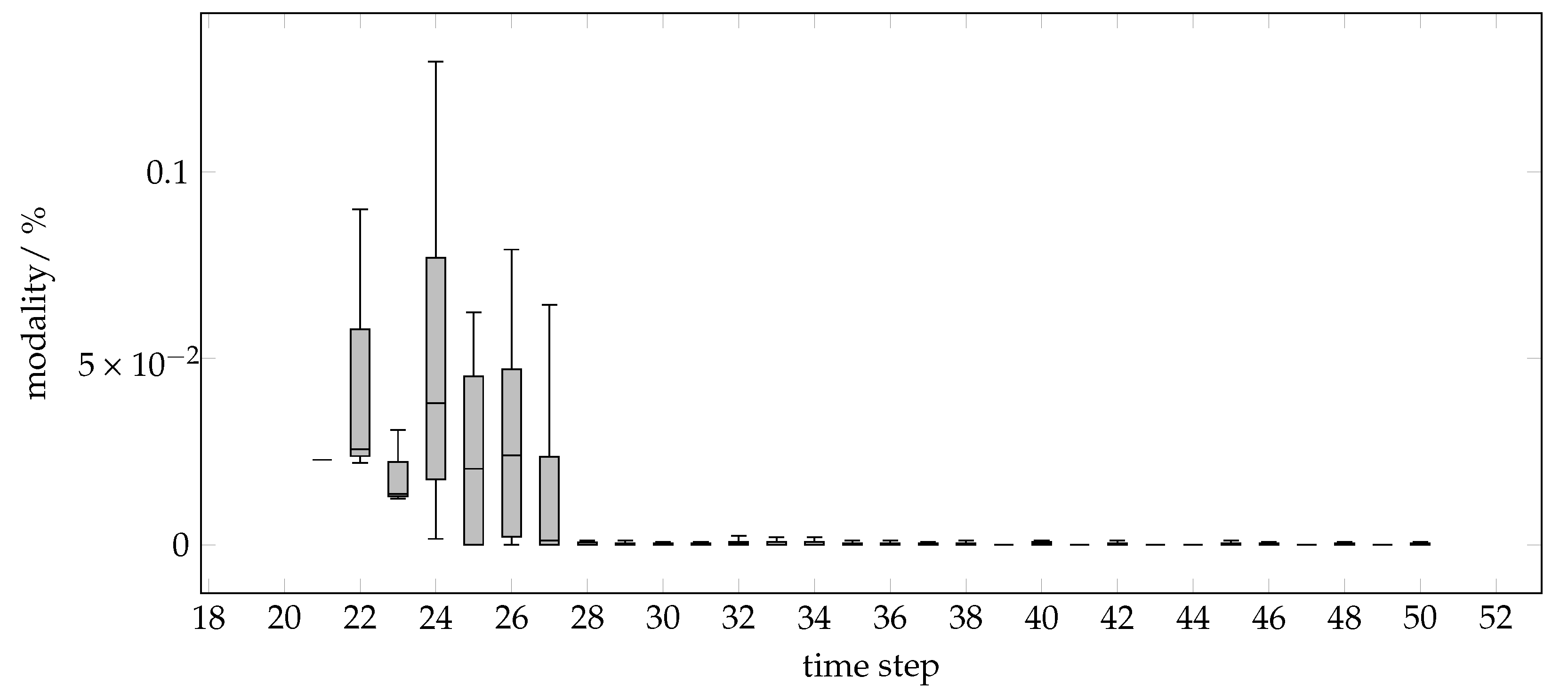
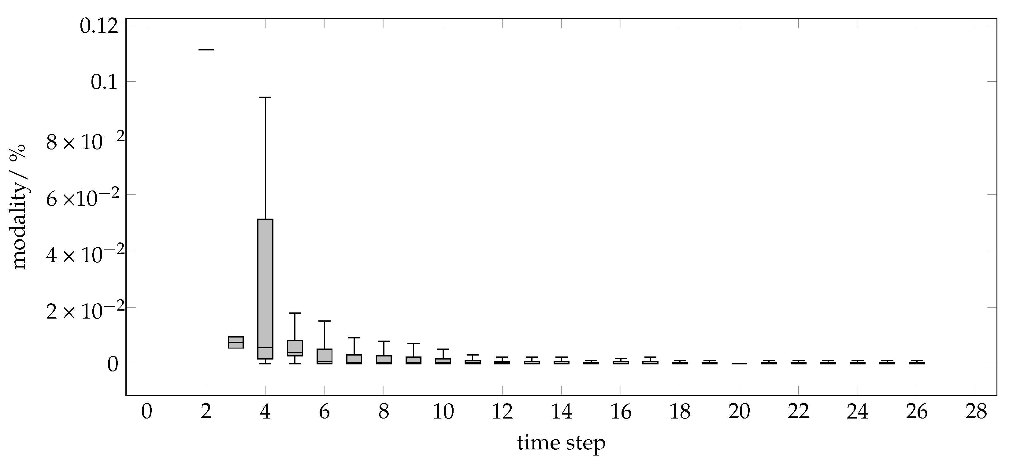
The rest of the paper is organized as follows. We start with a recap of both technologies that are combined into the distributed CGP. We describe the adaption of COHDA to CGP and how CMA-ES is adapted to suit the local optimization problem of an agent’s decision. The applicability and the effectiveness of the enumeration approach are demonstrated using problems from symbolic regression, n-parity problems, and classification problems. Finally, we demonstrate the superiority of the CMA-ES approach for larger problems. We justify the choice by analyzing the trace of the modality of the agent’s local optimization problems with a fitness landscape analysis. We conclude with a prospective view of further use cases and possible extensions.

2. Distributing Cartesian Genetic Programming

In CGP, computer programs are encoded as graph representations [39]. In general, CGP is an enhancement of a method that was originally developed for the use case of evolving digital circuits [40,41]. CGP already demonstrated its capabilities in synthesizing complex functions. Several different use cases from different fields have so far been scrutinized, for example, for image processing [42] or neural network training [4]. Moreover, some additions to CGP have been developed. Examples comprise recurrent CGP [23] (as in recurrent neural networks) or self-modifying CGP [43]. The authors in [33] used standard CGP. As the extension presented here improves the original approach in an internal sub-process, we also used standard CGP.
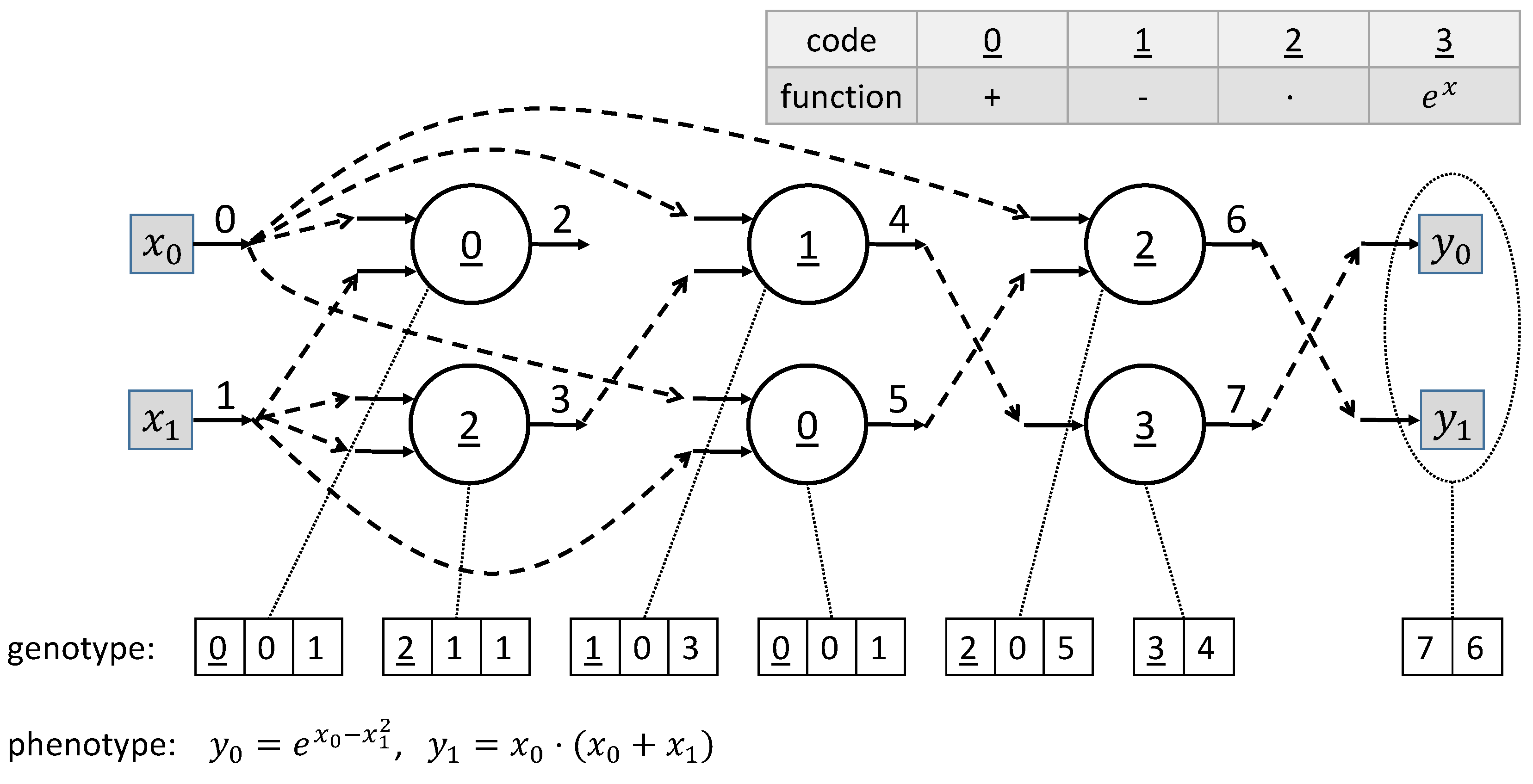
A chromosome in CGP comprises function-encoding genes and connection- and output-encoding genes. Together, they encode a computational graph (actually, a grid) that represents the executable program. The example in Figure 1 shows a graph with six computational nodes, two inputs, and also two outputs. The allele that encodes a function represents the index in an associated look-up table (from 0 ̲ to 3 ̲ in the example) with a list of all functions.
Each computation node is encoded by a gene sequence consisting of the function look-up index and the connected input (input into the system or output of another computation node). These are the parameters that are fed into the function. Hence, the total length of each function node gene sequence is n + 1 with n being the arity of the function plus one allele for the function index. The graph in standard CGP is an acyclic one. Parameters that are fed into a computation node may only be collected from nodes that have already been executed or from the inputs into the system. Thus, standard CGP works with a predefined execution order. Outputs can be connected to any computation node (representing the computation result of the output) or directly to any system input. Not all outputs of computational nodes are used as input for other functions. There might be no connections. Usually, many such unused computational nodes occur in evolved CGP [40] programs. These nodes are inactive, do not contribute to the encoded program’s output, and are not executed during the interpretation of the program. Thus, they do not cause any delay in computation.
Phenotypes are of variable length. In contrast, the size of the chromosome is static. As functions may have different arities, some genes may remain unused as input connections. Using an intermediate output of an inner node is also not mandatory. In this way, the fact that evolution is mainly responsible for rewiring makes CGP special.
COHDA has been introduced as a distributed multi-agent solution to distributed energy management problems [44]. Since then, it has been used for many different use cases. Examples include coalition structure formation [45], global optimization [38], trajectory optimization for unmanned air vehicles [46], or surplus distribution based on game theory [47].
In [33], COHDA has been used for distributing the evolution of Cartesian genetic programs. When COHDA is executed, each participating agent reacts to updated information from other agents. This is completed by adapting the own previous decision on a possible (local) solution candidate. In the original use case, COHDA agents represented a decentralized energy unit in distributed energy management. In this way, agents had to select an energy generation scheme for their own controlled energy unit. The selection had to be carried out such that it enables a group of energy-generation units to jointly fulfill an energy product (e.g.,  from some energy market) as well as they can. So, each agent had to decide on the local energy-generation profile only for a single generator. All decisions were always based on (intermediate) selected production schemes of other agents.
We start by we explaining the agent protocol that is the base algorithm for CGP program evolution.
In [36], COHDA was introduced to solve a problem known as predictive scheduling [48]. This is a problem from the smart grid domain and serves as an example here. COHDA works with an asynchronous iterative approximate best-response behavior, which means that all agents coordinate themselves by updating knowledge and exchanging information about each other. The agents make local decisions solely based on this information. The general protocol works in three repeatedly executed steps.
However, in the beginning, the agents are drawn together first by an artificial communication topology. As a first step, a small-world topology [49] has proven useful and is the most used topology. For this reason, we also use a small-world topology. Starting with an arbitrarily chosen agent and then passing it a message containing just the global objective, each agent repeatedly goes through three stages: perception, decision, and action (cf.  [50]).
  • Perception phase: In this first phase, the agent prepares for local decision-making. Each time the agent receives a message from one of the neighboring agents (which precedes the directed communication topology), the data that are contained in the message are included into their own knowledge base. The data that come with the message consist of the updated local decision of the agent that sent the message and the transient information on the decisions of other agents that led to the previous agent’s decision. After updating the local knowledge with the received information, usually, a local decision is made based on this information. In order to better escape local minima, agents may postpone a decision until more information has been collected [51].
  • Decision phase: Here, the agent has to conduct a local optimization to yield the best decision for its own local action that puts the coalition forward as best as possible. To complete this, each agent solves a low-dimensional part of the problem. The term “dimension”, in this context, can also refer to a sub-manifold containing low-dimensional local solutions as a fraction of a much higher-dimensional global search space. In the smart grid use case, for example, a local contribution to the global solution (the energy generation profile for a large group of independently working energy resources) consists of a many-dimensional real-valued vector describing the amount of generated energy per time interval for one single device. In the CGP case, a local solution would consist of a local chromosome encoding the functions and inputs of a single node. Other agents have made local decisions before, and, based on the gathered information about the (intermediate) local decisions of these agents, a solution candidate for the local (constrained) search space is sought. To this decision phase, we added CMA-ES for better local optimization.
  • Action phase: In the last stage, the agent compares the fitness of the best-found solution with the previous solution. For comparison, the global objective function is used. When the new solution has a better fitness (or a lower error, depending on the specific problem setting), the agent finally broadcasts a message containing its new local solution contribution together with everything it has learned from the other agents and their current local solution contributions (the decision base) to its immediate neighbors in the communication topology. Receiving agents then execute these three phases from scratch, leading probably to revised local solution contributions and thus to further improved overall solutions.
If an agent is not able to find a local solution contribution that improves the overall solution, no message is sent. If no agent can find any improvement, the process has reached at least the local optimum and eventually ceases because no more messages are sent.
After the system has produced a series of intermediate solutions, the heuristic eventually terminates in a state where all agents know an identical solution. This one is taken as the final solution of the heuristic. Properties such as guaranteed convergence and local optimality have been formally proven [44]. Moreover, after a short setup time, COHDA possesses the anytime property. Thus, the agent protocol may be stopped at any time with a valid (sub-optimal) solution, if necessary.
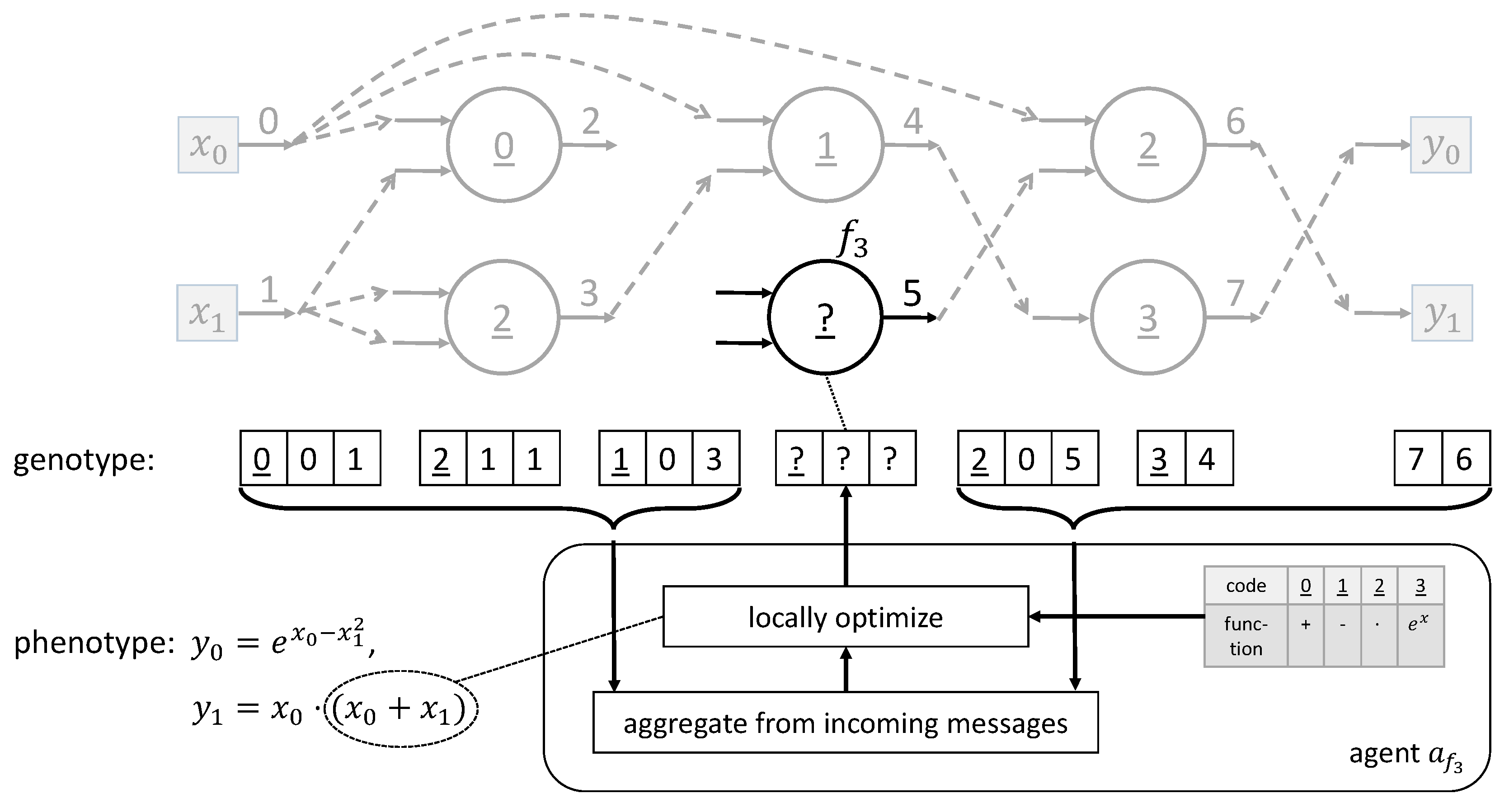
The agent approach can be adapted to CGP as follows. Each agent is responsible for a single node in the program graph. In general, there are two types of agents, the function node agents a f i responsible for the function node f i and the output agents a y j responsible for the output y j . The task of both agent types is rather similar but can be distinguished by the local search space. Each function node agent is responsible for exactly one node and thus internally just manages the code (look-up table address) of the function and the respective input addresses as a variable number of integers depending on the arity of the function. This list of integers is just one sub-chromosome of a complete solution. At the same time, every agent has some knowledge about the intermediate assignment of alleles to chromosomes of other agents. These are immutable for this agent. Together (their own gene set and the knowledge of others’ gene sets), the genotype of a complete solution, and, subsequently, a phenotype solution can be constructed by an agent.
If an agent that is responsible for a function node receives a message, it updates its own knowledge about the other agents. Each agent knows the most recent chromosomes from other agents. If newer information is received with the message, the outdated gene information is updated. In the case that such far unknown information arrives, additional genes are integrated into the agent’s own belief. After the data update, the agent has to make a decision about its own chromosome. This decision is a local optimization process previously solved by enumerating all of the solution candidates [33].
The known genes of the other agents are temporarily treated as fixed for the duration of the agent’s current decision-making. Each agent may make modifications only to its own chromosome. Nevertheless, the genes of the other agents may afterward again be altered by the respective agents as a reaction to previously made alterations. If an agent makes a new local decision, it solves for the global problem of finding a good genotype but may only mutate its own local chromosome. Figure 2 shows this situation as an example of the agent a f 3 that is responsible for the function node f 3 .
The optimization for finding the best local decision could, in general, be completed by any algorithm; e.g., by an evolution strategy. For the test cases in [33], the full enumeration of all solution candidates was sufficiently fast enough because each agent had just a rather limited set of choices. Nevertheless, for larger scenarios, the use of problem-specific heuristics has already been recommended in [33]. Constraints can easily be checked as the number of functions and the arity of each function are known to the agent. Currently, we set the number of rows in the graph to one (as in [33]). This convenient single-row representation has been shown to be no less effective [52] and has already been frequently used, e.g., in [53]. The levels-back parameter is set to the number of agents to allow input from all preceding nodes. Each agent knows its own index and may thus decide which other nodes (or program input) to choose as input for its own node.
As soon as the best local allele assignment has been found, the agent compares the solution quality with the quality of the previously found solution. If the new solution is better, messages are sent to neighboring agents. During our experiments, we found that it is advantageous to always send messages to the output agents in order to enable a more frequent update of the best output. The basic difference between the function and the output node agents is the local gene. The output agents just manage a single gene consisting of a single-integer allele that encodes the node that is connected to the respective output.
When no more agents can progress, no messages are sent, and the whole negotiation process finally ceases. Initially, COHDA was supposed to approach an often unknown optimum as closely as possible. For the CGP use case, on the other hand, it is also fine to drop out of the process if one agent, for the first time, finds a solution that fully satisfies a quality condition (i.e., the program does what it is supposed to do). Thus, we added an additional termination criterion. If an agent discovers a solution that constitutes a success, it sends a termination signal instead of a decision message and reports the found solution.

3. Evaluation

3.1. General Approach

For evaluation of the overall approach, The authors in [33] investigated three use cases: regression problems, the n-parity problem, and classification problems. We start with a recap of the results.

3.1.1. Regression

For comparison with the results achieved by the original CGP from [54], a symbolic regression of the following sixth order polynomial was used: x 6 2 x 4 + x 2 . The objective here is to evolve a program that produces the same output for the arbitrary input x. The function set that was used consisted of the four basic arithmetic operations: { + , , · , / } . For evaluation, 50 input values x were randomly chosen from the interval [ 1 , 1 ] , and x was the only input to the program. In the original approach, [54] gave also the constant 1.0 as additional input to the program. Previously, ephemeral constants had been used as well to support with solving the problem with GP [55]. Already in [33], it was observed that this additional help is not necessary, and so, we also refrained from using such auxiliary constructs.
For comparison, the following statistical measures as introduced by John Koza [56] were used. The cumulative probability of success for a budget of i objective evaluations is given by
P ( M , i ) = n success ( i ) n total ,
where n success denotes the number of successful runs with i objective function calls each, and n total denotes the total number of runs. M denotes the number of individuals. In our use case, M—although possibly interpretable as the number of agents—is of no use as the agent system works asynchronously and not in terms of generations with a constant number of evaluations per iteration. Instead, i was set to the total budget of the maximum number of objective function calls allowed by all of the agents together, and, thus, M was set to M : = 1 . This approach is consistent with the generalization in [57].
From the success rate, the mean number of independent runs required to achieve a minimum rate of success when the budget is fixed to a maximum of i evaluations per run can be derived. Let z denote the wanted success rate. Then,
R ( z ) = log ( 1 z ) log ( 1 P ( M , i ) )
gives the number of necessary runs. The computational effort I ( M , i , z ) = M · i · R ( z ) gives the number of individual function evaluations that must be performed to solve a problem to a proportion of z [57]. As i is a matter of parametrization, Koza defines the minimum computational effort as
I min ( M , z ) = min i M · R ( z ) .
Table 1 shows the comparison of results yielded from distributed CGP with the original results from [54]. The distributed approach shows competitiveness compared with the original results achieved with a genetic algorithm with a population size of 10, a uniform crossover (100% rate), and a 2% mutation. In [54], the number of maximum generations was set to 8000. This is not meaningful in asynchronous agent systems. In [33], the total number of evaluations was restricted to 80,000 (for 10 agents in total) instead. The confidence level was set to z = 0.99 .
Table 2 shows some results for several other symbolic regression problems.
Figure 3 explores the relation of the number of agents (and thus mainly the functional nodes) to the mean number of evaluations and to the length of the encoded phenotype solution (the number of active nodes). The experiment was conducted for the simple regression problem x 6 with 100 runs for each different number of agents. Although the mean number of active nodes (calculated only for successful runs) stays rather constant in Figure 3b, an unnecessarily high number of agents leads obviously to some outliers with a bloated phenotype. The mean number of evaluations also grows. Future improvements should address these issues, maybe by starting with a rather low number of agents and adding more agents only in the case that no further improvement to a solution is detected.

3.1.2. N-Parity

Evolving Boolean functions is a standard use case in evaluating genetic programming algorithms [58,59,60]. A special case is the even-n-parity problem [56]. The goal is to find a function that counts the number of ones of the given n bits using only Boolean expressions, returning TRUE if the number is even. In this way, a correct classification of arbitrary bit strings of a length n with an even number of ones is sought [61]. The input to the CGP program are the bits b 0 , , b n . The used function set for program evolution consists of the four Boolean functions { A N D , O R , N A N D , a n d N O R } . The Boolean even-n-parity function is seen as the most difficult Boolean function to evolve [56,62]. With standard GP, results for problem sizes up to n = 5 can be obtained [62]. For solving larger instances, techniques such as automatically defined functions [63] or extended function sets are needed [59]. Some results for the CGP programs evolved by COHDA are listed in Table 3. The number of agents and the total budget (for all agents together) are a result of sampling for the minimal computational effort (Equation (3)). Sampling has been carried out by grid search.
So far, distributed CGP had been trained for up to n = 5 . For smaller instances of the problem, different numbers of agents (the computation nodes) were tested as well. Obviously, having larger chromosomes (the number of agents in our case), as stated in [64], is not always advantageous—at least in the distributed case.

3.1.3. Classification

Finally, a real-world problem from the energy domain was used. The distributed approach was tested on a classification problem known as flexibility modeling [65] and adapted. The goal is to correctly classify the energy-generation profiles x R d with x i , denoting the generated amount of energy during the ith time interval for a given, specific energy resource. A generation profile x can either be feasible (meaning it can be operated by the energy resource without violating any technical constraint) or not. This problem is often modeled as a one-class classification problem [66].
Solutions using support vector machines (SVM) or support vector data description (SVDD) as a classifier can, for example, be found in [67,68]. The approach was compared with SVDD [69]. The classifiers are trained using a set of feasible generation profiles that is generated using an appropriate simulation model of the energy resource. The authors in [33] used the model of a co-generation plant (CHP). This model comprises a micro CHP with 4.7 kW of rated electrical power (12.6 kW thermal power) bundled with a thermal buffer store. Constraints restrict the power band, buffer charging, gradients, min. on and off times, and satisfaction of thermal demand. Thermal demand is a subject to simulate the losses of a detached house according to given weather profiles. For each agent, the CHP model is individually (randomly) configured with a state of charge, weather condition, temperature range, allowed operation gradients, and similar variables [47].
The goal was to evolve a program that obtains d values that represent the amount of energy x = ( x 1 , , x d ) as inputs and outputs of y < 0 , if the profile is infeasible to operate for the energy resource, or y 0 , in the case that the profile is feasible and can thus be operated by the CHP. For evaluation, a training set of 1000 generation profiles (50% feasible) that was generated by the simulation model was used. The function set was: { + , , · , / , AND , OR , NOT , XOR , = , < , > , IF   THEN   ELSE , 0 , 1 , 2 } , with 0, 1, and 2 denoting constants (nullary functions).
For evaluation and for comparing the performance of the the classifiers, we used the classification accuracy. Evaluation during CGP evolution was completed using 1000 training instances to calculate the confusion matrix and, finally, the achieved accuracy. The SVDD classifier was trained with 1000 feasible instances. After the classifier program has been evolved, we compared the CGP classifier with the SVDD classifier using 100 times a test set of 1000 newly generated, thus far unseen generation profile instances from identically parameterized simulation models (the same sets for both classifiers, respectively). Table 4 shows the results for the different dimensions d of the generation profile.
Although all CGP results are slightly worse than those of SVDD, the achieved accuracy is still estimable. The training accuracy denotes the best fitness that has been achieved during several test runs of program evolution. The best-found programs were then been applied to the different unseen test sets generated for the newly instantiated CHP models. This generalization ability is compared between CGP and SVDD by their respective mean accuracies. Another interesting observation can be seen in the following example phenotype for eight-dimensional generation profiles as input:
y = + ( ( x 1 , x 3 ) , IF ( x 7 , ( / ( 2.0 , ( AND ( x 0 , ( / ( x 0 , x 7 ) , x 7 ) ) , ( x 1 , x 3 ) ) ) , + ( / ( x 6 , x 7 ) , / ( x 7 , x 6 ) ) ) , x 0 ) ) .
Obviously, not all inputs are always of interest for classification as some are constantly omitted. These were always the same ones in different evolved programs. This fact is also reflected by the just marginally growing number of agents compared to the faster-growing dimensionality of the problem. Such identification of the smaller intrinsic dimension is an extra for the CGP program not provided by classifiers such as SVDD.

3.2. CMA-ES for Optimizing Local Agent Decisions

The covariance matrix adaption evolution strategy [70,71] is well known as an evolution strategy for solving multi-modal black-box problems by using lessons that have been learned from previously seen successful evolution steps for the improvement of future operations. A new population of solution candidates is sampled from a multivariate normal distribution N ( 0 , C ) with the covariance matrix C . This covariance matrix is adapted at the end of each iteration such that it maximizes the generation of improving steps according to previously seen distributions for good steps. The method learns a second-order model of the objective function and exploits it for structure information and for reducing the calls of objective evaluations. Such behavior renders this algorithm especially useful for our purpose as it is used as an inner part (optimizing the local decision of an agent) of a bi-level approach. In this way, CMA-ES is used for calculating the objective of an outer optimization (the agent negotiations). Thus, using as few objective evaluations as possible is advantageous for our use case.
An a priori parametrization with structure knowledge of the problem by the user is not necessary as if the method is adapting itself without supervision. A good introduction to CMA-ES can be found, for example, in [72].
CMA-ES is used for solving the internal optimization problem that arises when an agent has to decide on the best allele combination for the local sub-chromosome that encodes the function controlled by that agent. Thus, the dimension of the problem that has to be solved by CMA-ES is determined by the number of genes in the chromosome, which is rather small compared to the overall number of genes of the global problem that is used for evaluation. Thus, CMA-ES is expected to still work rather quickly and not to suffer from performance degradation due to the huge matrix computations caused by high-dimensional problem instances. In the following, we follow [73,74] with our explanations.
We consider the aforementioned agent negotiation with a stage in which each agent has to search the individual allele configuration for a single node. Thus, the individual feasible set of indices for function encoding and wiring of other outputs to this input for the best option (according to the given objectives) must be found. This search constitutes a local optimization problem. As this smaller sub-problem is a local one, as seen from the agent’s perspective, there is no need to harness a distributed solving strategy.
As this local optimization is part of the exterior agent negotiation process, and because it is therefore called many times, a heuristic that uses only a small number of objective evaluations is advantageous. CMA-ES is well known for this characteristic [72]. The constraints of this optimization problem are rather simple box constraints and, thus, easy to handle.
In each iteration g of CMA-ES, a multivariate distribution is sampled in order to generate a new offspring solution population in the σ -vicinity of good parent solutions with the mean m:
x k ( g + 1 ) m ( g ) + σ ( g ) N ( 0 , C ( g ) ) , k = 1 , , λ .
This sampling is suitable for continuous problems. To be able to use CMA-ES for our discrete problem, we allowed continuous alleles and scaled them back to discrete values prior to their assignment to genes in the sub-chromosome. Additionally, we restricted the range to [ 0 , 1 [ :
x k ( g + 1 ) = x k ( g + 1 ) mod 1 , x k ( g + 1 ) 1 ( x k ( g + 1 ) mod 1 ) + 1 , x k ( g + 1 ) < 0 .
C ( g ) R n × n constitutes the covariance matrix of the search distribution at a generation (iteration) g with an overall standard deviation σ ( g ) that can also be interpreted in terms of an adaptive (multivariate) step size. The step size is adapted individually for each dimension to support and favor the direction in which fast improvement can be expected according to the formerly seen results. The mean of the multivariate distribution is denoted by m ( g ) ; λ 2 denotes the population size.
The new mean m ( g + 1 ) for generating a sample of the next generation in CMA-ES is calculated as the weighted average
m ( g + 1 ) = i = 1 μ w i x i : λ ( g + 1 ) , w i = 1 , w i > 0 ,
of the best (in terms of the objective function evaluation) individuals form the current sample x i ( g ) , , x λ ( g ) .
In order to make the above relaxed continuous genotype solution candidates discrete again, we introduce a decoder mapping to the respective phenotype (example of agent a f i ):
γ = x k , i ( g + 1 ) · | F | i = 0 x k , i ( g + 1 ) · index ( a f i ) i > 0 , 0 I < 1 + max arity ( F )
where | F | denotes the number of functions in the function set F, index ( a f i ) denotes the number of agents that are ahead of agent a f i (only from these may the input be taken), and max arity ( F ) denotes the maximum arity of all functions in the set. In this way, the solution candidate is scaled back to a valid discrete genotype.
In our case, the genotype consists of a sub-chromosome with the zeroth gene encoding the function and genes 1 to max arity ( F ) + 1 encoding the wiring with the previous (in the calculation line). Functions with an arity lower than the maximum arity do not use all wirings. This approach is in line with [75].
Ranking is now carried out by
f ( γ ( x 1 : λ ( g ) ) , κ ) , , f ( γ ( x λ : λ ( g ) ) , κ ) , λ μ ,
to define x i : λ ( g ) as the ith-ranked best individual. Please note that for evaluation, the global objective is used. The evaluation of the global objective takes the individual sub-chromosomes of all agents and combines them. Thus, κ in Equation (9) denotes the current working memory of the agent. κ contains the temporarily fixed alleles of the other agents (so far known from the perception phase).
Finally, the covariance matrix is updated as usual and is also based on the decoder-based ranking Equation (9):
C μ ( g + 1 ) = i = 1 μ w i x i : λ ( g + 1 ) m ( g ) x i : λ ( g + 1 ) m ( g ) .
CMA-ES has a set of parameters that can be tweaked to some degree for a problem-specific adaption. Nevertheless, the default values that are applicable for a wide range of problems are usually available. For our experiments, we used the following default settings for the CMA-ES part. The (external) strategy parameters are λ , μ , w i = 1 μ , controlling selection and recombination; c σ and d σ controlling the step size; and c c and μ c o v controlling the covariance matrix adaption. We have chosen to set these values after [72]:
λ = 4 + 3 ln n , μ = λ 2 ,
w i = ln ( λ 2 + 0.5 ) ln i μ j = 1 λ 2 + 0.5 ) ln i , i = 1 , , μ
C c = 4 n + 4 , μ c o v = μ e f f ,
C c o v = 1 μ c o v 2 ( n + 2 ) 2 + 1 1 μ c o v min 1 , 2 μ c o v 1 ( n + 2 ) 2 + μ c o v .
An in-depth discussion of these parameters is also given in [76]. These settings are specific to the dimension N of the objective function. In our case, N = 1 + max arity ( F ) is related to the maximum arity of all functions in the function set plus one gene for encoding the function itself. Thus, the dimensionallity stays rather small. Hence, CMA-ES will not suffer from large matrix calculations for updating the covariance matrix as in high-dimensional problems.

3.3. Results

For the evaluation of the CMA-ES approach, we used the classification use case described above, as this is the most practically relevant use case from [33]. In order to make the problem more severe, we added five NOP to the function set, causing no harm to the result but making the search space exponentially larger. In addition, we used more agents to further increase the search space (due to more wiring choices). This is also quite realistic for the use case of an agent swarm that is supposed to learn how to solve new, unseen problems. An agent may offer abilities and functions that are of no use for solving the problem but increase the search space.
As there is no known minimum in this optimization problem, we chose to stop the process as soon as the objective value of 0.18 has been found. This value has been empirically found. We observed that, once a CGP program with an objective value of less than or equal to 0.18 has been found, the program shows a sufficiently good performance in classification. The absolute number of objective evaluations of all agents was counted to calculate Koza’s minimum effort statistics.
The results showed that full enumeration—except for very small problem instances—had to be stopped at some point (we chose 5 million evaluations) without a valid result. Table 5 shows the result for a small four-dimensional classification problem.
This example already shows the vast improvement of CMA-ES over full enumeration. The minimum computational effort that the agents (in total) needed with CMA-ES is more than 300 times smaller than with full enumeration. For larger examples, the full enumeration approach was not at all able to obtain a sufficiently good result with a reasonable budget for the objective evaluations. For this reason, we omitted full enumeration in the remaining results. Table 6 and Table 7 finally show some results for larger classification problems of CMA-ES only.

3.4. Analysis

Finally, we analyzed the individual complexity that the agents face during different episodes of the negotiation. This complexity is not constant. It depends on the previous choices of all other agents. If it is an agent’s turn to make a decision—i.e., to optimize its own function choice, including the wiring of the parameters to the other agent’s functions—the fitness landscape is defined as follows
F = ( S , f , d ) ,
with the search space S, which always stays the same (the set of all combinations of the functions with the allowed parameter wirings) and the neighborhood definition d. For our research, we used the following neighborhood:
x i k + 1 = x i k + 1 if r 1 3 x i k if 1 3 < r 2 3 x i k 1 otherwise , 1 i d .
Here, x k + 1 denotes a neighboring solution that is generated from a solution candidate x k . The random variable r is uniformly randomly sampled from the interval [ 0 , 1 ] .
In this way, each allele is increased by one, decreased by one or stays the same with a likelihood of 1/3 each. The element that changes in the landscape definition F is the objective function f. The objective f is still defined as described above for the classification use case. The classification accuracy (which is used for f) is calculated using the performance of a solution candidate on different so-far unseen classification instances. However, this performance highly depends on the decisions of all other agents. Thus, the fitness landscape varies with each call of the decision method of an agent.
The analysis then was performed as follows. Prior to each decision method call, the modality (as a measure of ruggedness) of the local problem of each agent was calculated. To complete this, we followed the method of [77]. First, we generated a series of fitness values by using a random path of the solution candidates on the fitness landscape. To generate the random path, the neighborhood relation d from Equation (16) was used. For each solution candidate along the generated path, the fitness can be calculated using the objective function with the fixed parts of the other agents. We can then tokenize the series of all subsequent fitness values to a sequence of tokens encoding uphill, downhill, or flat episodes. The relation of the length of the shortest possible token string (containing up, down, and flat tokens) to the length of the original path or series of fitness values then gives a measure for the modality ρ [ 0 , 1 ] . ρ = 0 denotes a completely flat fitness landscape; ρ = 1 , on the other hand, denotes the maximum number of local optima that fit into a path of the given length.
This modality is calculated for each local decision of each agent. Figure 4 shows an example result for a first, simple instance of the classification problem. Here, we looked at a four-dimensional classification problem and used 20 agents for evolving a program that does the classification of CHP schedule feasibility. Time-steps (as a unit for time), in this case, are an artificial measure. The multi-agent systems work asynchronously, but, we can maintain an artificial clock tick that could be interpreted as a unit of time (second, millisecond, …) but, in fact, has no practical meaning here except for ordering the events.
The experiment has been repeated four times, as depicted in Figure 4a–d. We see that the modality varies over time and becomes lower toward the end of the evolution process. The latter fact is not immediately clear. Although toward the end more and more agents fix their local result because they are unable to find any further improvement, it is not clear why this should make the search for the remaining agents easier.
Nevertheless, this seems to be a general pattern. Figure 5, Figure 6 and Figure 7 show some more examples of 96-dimensional classification problem instances. These figures show the same general pattern. Moreover, it seems that if the number of agents is increased, the phase of high modality in local optimization moves to earlier stages. The number of agents varies from 50 (used for the result in Figure 5) to 200 (which is already way too many; see Figure 7).
We can conclude two things:
1
The choice of CMA-ES as an algorithm that adapts without supervision to different problem instances with different characteristics was good because the modality of the local optimization problems that the agents have to solve comprises a wide range of modalities.
2
It seems worthwhile to conduct a larger and more thorough fitness landscape analysis in order to develop situation-aware and adaptive local decision support for the agents.
Thus, future work will address a fitness landscape-aware selection of different local optimization techniques for the agents.

4. Conclusions

We presented the adaption of a distributed optimization heuristic protocol for Cartesian genetic programming and an extension using CMA-ES for improving local agent decisions. By decomposing the evolution on an algorithmic level, it becomes possible to distribute the nodes and regard the evolution process as a parallel, asynchronous execution of an individual coordinate’s descent.
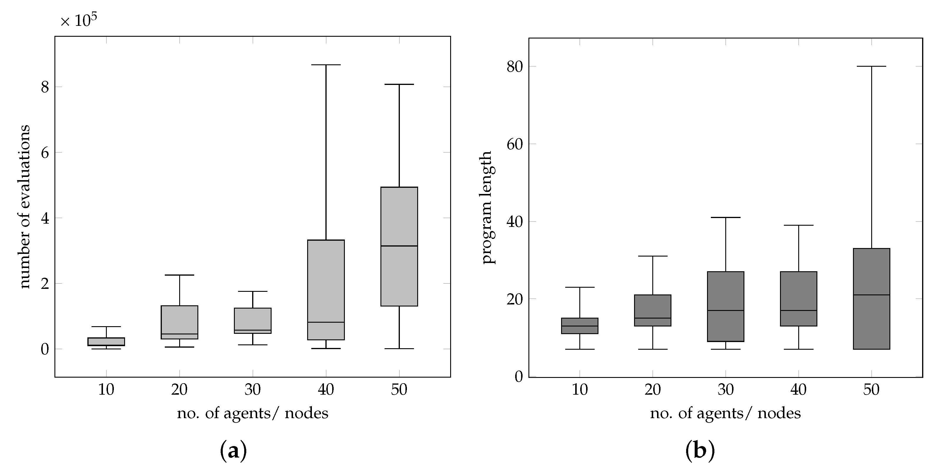
The results show that the distributed approach is competitive with regard to the evolved programs. This holds true for the solution quality as well as for the computational effort and for smaller tasks even with the full enumeration approach. A speed-up by parallel execution becomes possible and has been increased significantly here. With the extension via CMA-ES for agent-internal optimization during decision-making, the computational effort has dropped significantly, even for larger problem instances. Another advantage is the ability to distribute the computational burden. Moreover, the distributed evolution of programs enables seamless integration into distributed applications, in addition to using the example of the smart grid.
Agent-based Cartesian genetic programming constitutes a universal means to execute cooperative planning among individually acting entities. Future work will now lean toward distributed use cases. Another advantage is that different nodes may have different function sets in case they represent real-world nodes with different capabilities.
So far, we considered only the original standard CGP. Extensions such as recurrent CGP can be integrated right away now. These extensions affect basic interpretation (some also affect the execution of the phenotype) and can thus be evolved by the same distributed approach. Only an adaption of the possible choices of other agents’ output as input for its own node is necessary. In the same way, different levels-back parameterizations can be easily handled.
Further improvements are expected when agents are equipped with intelligent rules for choosing from different decision methods; i.e., optimization methods (CMA-ES, full enumeration, others) should be chosen ad hoc from a set of different methods according to the current individual’s situation.
However, even with this initial setting that has been scrutinized in this contribution for making a swarm of individually acting agents learn problem-solving via distributed CGP, the results are already very promising. Agents capable of combining individual skills to solve so-far unseen problems without any central algorithm are a major building block for large-scale future autonomous cyber-physical systems.

Author Contributions

Conceptualization, J.B. and S.L.; methodology, J.B.; software, J.B. and S.L.; validation, J.B. and S.L.; formal analysis, J.B.; investigation, J.B. and S.L.; resources, S.L.; data curation, J.B. and S.L.; writing—original draft preparation, J.B.; writing—review and editing, S.L.; visualization, J.B. All authors have read and agreed to the published version of the manuscript.

Funding

This research received no external funding.

Informed Consent Statement

Not applicable.

Data Availability Statement

An implementation of the used COHDA algorithm can be found at https://gitlab.com/mango-agents/ (accessed on 19 February 2023).

Conflicts of Interest

The authors declare no conflict of interest.

References

  1. Miller, J.F. An empirical study of the efficiency of learning boolean functions using a cartesian genetic programming approach. In Proceedings of the Genetic and Evolutionary Computation Conference, Orlando, FL, USA, 13–17 July 1999; Volume 2, pp. 1135–1142. [Google Scholar]
  2. Miller, J.F. Cartesian genetic programming: Its status and future. Genet. Program. Evolvable Mach. 2020, 21, 129–168. [Google Scholar] [CrossRef] [Green Version]
  3. Manazir, A.; Raza, K. Recent developments in cartesian genetic programming and its variants. ACM Comput. Surv. (CSUR) 2019, 51, 1–29. [Google Scholar] [CrossRef]
  4. Khan, M.M.; Ahmad, A.M.; Khan, G.M.; Miller, J.F. Fast learning neural networks using cartesian genetic programming. Neurocomputing 2013, 121, 274–289. [Google Scholar] [CrossRef]
  5. Miller, J.F.; Mohid, M. Function Optimization Using Cartesian Genetic Programming. In Proceedings of the 15th Annual Conference Companion on Genetic and Evolutionary Computation, Amsterdam, The Netherlands, 6–10 July 2013; Association for Computing Machinery: New York, NY, USA, 2013. GECCO ’13 Companion. pp. 147–148. [Google Scholar] [CrossRef]
  6. Clegg, J.; Walker, J.A.; Miller, J.F. A new crossover technique for cartesian genetic programming. In Proceedings of the 9th Annual Conference on Genetic and Evolutionary Computation, London, UK, 7–11 July 2007; pp. 1580–1587. [Google Scholar]
  7. Calvaresi, D.; Appoggetti, K.; Lustrissimini, L.; Marinoni, M.; Sernani, P.; Dragoni, A.F.; Schumacher, M. Multi-Agent Systems’ Negotiation Protocols for Cyber-Physical Systems: Results from a Systematic Literature Review. In Proceedings of the ICAART (1), Funchal, Portugal, 16–18 January 2018; pp. 224–235. [Google Scholar]
  8. Zhu, Q.; Bushnell, L.; Başar, T. Resilient distributed control of multi-agent cyber-physical systems. In Control of Cyber-Physical Systems; Springer: Berlin/Heidelberg, Germany, 2013; pp. 301–316. [Google Scholar]
  9. Nieße, A.; Lehnhoff, S.; Tröschel, M.; Uslar, M.; Wissing, C.; Appelrath, H.J.; Sonnenschein, M. Market-based self-organized provision of active power and ancillary services: An agent-based approach for Smart Distribution Grids. In Proceedings of the 2012 Complexity in Engineering (COMPENG), Aachen, Germany, 11–13 June 2012; pp. 1–5. [Google Scholar] [CrossRef]
  10. Bremer, J. Learning to Optimize. In Recent Advances in Computational Optimization: Results of the Workshop on Computational Optimization WCO 2021; Fidanova, S., Ed.; Springer International Publishing: Cham, Switzerland, 2022; pp. 1–19. [Google Scholar] [CrossRef]
  11. Jipp, M.; Ackerman, P.L. The Impact of Higher Levels of Automation on Performance and Situation Awareness. J. Cogn. Eng. Decis. Mak. 2016, 10, 138–166. [Google Scholar] [CrossRef]
  12. Sheridan, T.B.; Parasuraman, R. Human-Automation Interaction. Rev. Hum. Factors Ergon. 2016, 1, 89–129. [Google Scholar] [CrossRef]
  13. European Commission. Draft Ethics Guidelines for Trustworthy AI; Technical Report; European Commission: Brussels, Belgium, 2018. [Google Scholar]
  14. Rapp, B.; Solsbach, A.; Mahmoud, T.; Memari, A.; Bremer, J. IT-for-Green: Next Generation CEMIS for Environmental, Energy and Resource Management. In Proceedings of the EnviroInfo 2011–Innovations in Sharing Environmental Observation and Information, Proceedings of the 25th EnviroInfo Conference ‘Environmental Informatics’, Ispra, Italy, 5–7 October 2011; Pillmann, W., Schade, S., Smits, P., Eds.; Shaker Verlag: Herzogenrath, Germany, 2011; pp. 573–581. [Google Scholar]
  15. Gholami, M.; Pilloni, A.; Pisano, A.; Sanai Dashti, Z.A.; Usai, E. Robust Consensus-Based Secondary Voltage Restoration of Inverter-Based Islanded Microgrids with Delayed Communications. In Proceedings of the 2018 IEEE Conference on Decision and Control (CDC), Miami Beach, FL, USA, 17–19 December 2018; IEEE Press: Manhattan, NY, USA, 2018; pp. 811–816. [Google Scholar] [CrossRef]
  16. Gordon, M.A.; Vargas, F.J.; Peters, A.A.; Maass, A.I. Platoon Stability Conditions Under Inter-vehicle Additive Noisy Communication Channels. IFAC-PapersOnLine 2020, 53, 3150–3155. [Google Scholar] [CrossRef]
  17. Coppola, A.; Lui, D.G.; Petrillo, A.; Santini, S. Cooperative driving of heterogeneous uncertain nonlinear connected and autonomous vehicles via distributed switching robust PID-like control. Inf. Sci. 2023, 625, 277–298. [Google Scholar] [CrossRef]
  18. Platzer, A. The logical path to autonomous cyber-physical systems. In Proceedings of the International Conference on Quantitative Evaluation of Systems, Glasgow, UK, 9–12 September 2019; Springer: Berlin/Heidelberg, Germany, 2019; pp. 25–33. [Google Scholar]
  19. McKee, D.W.; Clement, S.J.; Almutairi, J.; Xu, J. Survey of advances and challenges in intelligent autonomy for distributed cyber-physical systems. CAAI Trans. Intell. Technol. 2018, 3, 75–82. [Google Scholar] [CrossRef]
  20. Collier, J. Fundamental properties of self-organization. Causality Emerg. Self-Organ. 2003, 287–302. [Google Scholar]
  21. Parzyjegla, H.; Schröter, A.; Seib, E.; Holzapfel, S.; Wander, M.; Richling, J.; Wacker, A.; Heiß, H.U.; Mühl, G.; Weis, T. Model-driven development of self-organising control applications. In Organic Computing–A Paradigm Shift for Complex Systems; Springer: Berlin/Heidelberg, Germany, 2011; pp. 131–144. [Google Scholar]
  22. Bremer, J.; Lehnhoff, S. Towards Evolutionary Emergence. Ann. Comput. Sci. Inf. Syst. 2021, 26, 55–60. [Google Scholar]
  23. Turner, A.J.; Miller, J.F. Recurrent Cartesian Genetic Programming. In Proceedings of the Parallel Problem Solving from Nature–PPSN XIII, Ljubljana, Slovenia, 13–17 September 2014; Bartz-Beielstein, T., Branke, J., Filipič, B., Smith, J., Eds.; Springer International Publishing: Cham, Switzerland, 2014; pp. 476–486. [Google Scholar]
  24. Goldman, B.W.; Punch, W.F. Reducing wasted evaluations in cartesian genetic programming. In Proceedings of the European Conference on Genetic Programming, 2013, Vienna, Austria, 3–5 April 2013; Springer: Berlin/Heidelberg, Germany, 2013; pp. 61–72. [Google Scholar]
  25. Walker, J.A.; Völk, K.; Smith, S.L.; Miller, J.F. Parallel evolution using multi-chromosome cartesian genetic programming. Genet. Program. Evolvable Mach. 2009, 10, 417. [Google Scholar] [CrossRef]
  26. Poli, R. Parallel Distributed Genetic Programming; University of Birmingham, Cognitive Science Research Centre: Birmingham, UK, 1996. [Google Scholar]
  27. Liu, Z.; Zhan, X.; Han, T.; Yan, H. Distributed Adaptive Finite-Time Bipartite Containment Control of Linear Multi-Agent Systems. IEEE Trans. Circuits Syst. II Express Briefs 2022, 69, 4354–4358. [Google Scholar] [CrossRef]
  28. Liu, G.; Liang, H.; Pan, Y.; Ahn, C.K. Antagonistic Interaction-Based Bipartite Consensus Control for Heterogeneous Networked Systems. IEEE Trans. Syst. Man Cybern. Syst. 2023, 53, 71–81. [Google Scholar] [CrossRef]
  29. Lui, D.G.; Petrillo, A.; Santini, S. Bipartite Tracking Consensus for High-Order Heterogeneous Uncertain Nonlinear Multi-Agent Systems With Unknown Leader Dynamics via Adaptive Fully-Distributed PID Control. IEEE Trans. Netw. Sci. Eng. 2023, 10, 1131–1142. [Google Scholar] [CrossRef]
  30. Yang, L.; Li, X.; Sun, M.; Sun, C. Hybrid Policy-based Reinforcement Learning of Adaptive Energy Management for the Energy Transmission-constrained Island Group. IEEE Trans. Ind. Inform. 2023, 1–12. [Google Scholar] [CrossRef]
  31. Zhang, N.; Sun, Q.; Yang, L.; Li, Y. Event-Triggered Distributed Hybrid Control Scheme for the Integrated Energy System. IEEE Trans. Ind. Inform. 2022, 18, 835–846. [Google Scholar] [CrossRef]
  32. Cerquides, J.; Farinelli, A.; Meseguer, P.; Ramchurn, S.D. A Tutorial on Optimization for Multi-Agent Systems. Comput. J. 2013, 57, 799–824. [Google Scholar] [CrossRef] [Green Version]
  33. Bremer, J.; Lehnhoff, S. Fully Distributed Cartesian Genetic Programming. In Proceedings of the Advances in Practical Applications of Agents, Multi-Agent Systems, and Complex Systems Simulation, The PAAMS Collection, L’Aquila, Italy, 13–15 July 2022; Dignum, F., Mathieu, P., Corchado, J.M., De La Prieta, F., Eds.; Springer International Publishing: Cham, Switzerland, 2022; pp. 36–49. [Google Scholar]
  34. Talbi, E.G. Metaheuristics: From Design to Implementation; John Wiley & Sons: Hoboken, NJ, USA, 2009; Volume 74. [Google Scholar]
  35. Hinrichs, C.; Vogel, U.; Sonnenschein, M. Approaching Decentralized Demand Side Management via Self-Organizing Agents. In Proceedings of the ATES Workshop, Proceedings of 10th Int. Conf. on Autonomous Agents and Multiagent Systems (AAMAS 2011), Taipei, Taiwan, 2–6 May 2011. [Google Scholar]
  36. Hinrichs, C.; Sonnenschein, M.; Lehnhoff, S. Evaluation of a Self-Organizing Heuristic for Interdependent Distributed Search Spaces. In Proceedings of the International Conference on Agents and Artificial Intelligence (ICAART 2013), Barcelona, Spain, 15–18 February 2013; Filipe, J., Fred, A.L.N., Eds.; SciTePress: Setúbal, Portugal, 2013; Volume 1, pp. 25–34. [Google Scholar] [CrossRef]
  37. Potter, M.A.; Jong, K.A.D. Cooperative coevolution: An architecture for evolving coadapted subcomponents. Evol. Comput. 2000, 8, 1–29. [Google Scholar] [CrossRef]
  38. Bremer, J.; Lehnhoff, S. The Effect of Laziness on Agents for Large Scale Global Optimization. In Proceedings of the Agents and Artificial Intelligence, Prague, Czech Republic, 19–21 February 2019; van den Herik, J., Rocha, A.P., Steels, L., Eds.; Springer International Publishing: Cham, Switzerland, 2019; pp. 317–337. [Google Scholar]
  39. Sotto, L.F.D.P.; Kaufmann, P.; Atkinson, T.; Kalkreuth, R.; Basgalupp, M.P. A Study on Graph Representations for Genetic Programming. In Proceedings of the 2020 Genetic and Evolutionary Computation Conference, Cancún, Mexico, 8–12 July 2020; Association for Computing Machinery: New York, NY, USA, 2020; pp. 931–939. [Google Scholar] [CrossRef]
  40. Miller, J. Cartesian Genetic Programming; Springer: Berlin/Heidelberg, Germany, 2003; Volume 4. [Google Scholar] [CrossRef]
  41. Miller, J.F.; Thomson, P.; Fogarty, T. Designing electronic circuits using evolutionary algorithms. arithmetic circuits: A case study. In Genetic Algorithms and Evolution Strategies in Engineering and Computer Science; John Wiley & Sons: Hoboken, NJ, USA, 1997; pp. 105–131. [Google Scholar]
  42. Harding, S.; Leitner, J.; Schmidhuber, J. Cartesian genetic programming for image processing. In Genetic Programming Theory and Practice X; Springer: Berlin/Heidelberg, Germany, 2013; pp. 31–44. [Google Scholar]
  43. Harding, S.; Banzhaf, W.; Miller, J.F. A survey of self modifying cartesian genetic programming. In Genetic Programming Theory and Practice VIII; Springer: Berlin/Heidelberg, Germany, 2011; pp. 91–107. [Google Scholar]
  44. Hinrichs, C.; Sonnenschein, M. A distributed combinatorial optimisation heuristic for the scheduling of energy resources represented by self-interested agents. Int. J. Bio-Inspired Comput. 2017, 10, 69–78. [Google Scholar] [CrossRef]
  45. Bremer, J.; Lehnhoff, S. Decentralized Coalition Formation with Agent-based Combinatorial Heuristics. ADCAIJ Adv. Distrib. Comput. Artif. Intell. J. 2017, 6, 29–44. [Google Scholar] [CrossRef] [Green Version]
  46. Tong, B.; Liu, Q.; Dai, C.; Jia, Z. A Decentralized Multiple MAV Collision Avoidance Trajectory Planning Method. In Proceedings of the 2020 Chinese Automation Congress (CAC), Shanghai, China, 6–8 November 2020; pp. 1545–1552. [Google Scholar] [CrossRef]
  47. Bremer, J.; Lehnhoff, S. Decentralized Surplus Distribution Estimation with Weighted k-Majority Voting Games. In Highlights of Practical Applications of Cyber-Physical Multi-Agent Systems, Proceedings of the International Workshops of PAAMS 2017, Porto, Portugal, 21–23 June 2017; Bajo, J., Vale, Z., Hallenborg, K., Rocha, A.P., Mathieu, P., Pawlewski, P., Del Val, E., Novais, P., Lopes, F., Duque Méndez, N.D., et al., Eds.; Springer International Publishing: Cham, Switzerland, 2017; pp. 327–339. [Google Scholar] [CrossRef]
  48. Sonnenschein, M.; Lünsdorf, O.; Bremer, J.; Tröschel, M. Decentralized Control of Units in Smart Grids for the Support of Renewable Energy Supply. Environ. Impact Assess. Rev. 2015, 52, 40–52. [Google Scholar] [CrossRef]
  49. Watts, D.; Strogatz, S. Collective dynamics of ’small-world’ networks. Nature 1998, 440–442. [Google Scholar] [CrossRef] [PubMed]
  50. Nieße, A.; Beer, S.; Bremer, J.; Hinrichs, C.; Lünsdorf, O.; Sonnenschein, M. Conjoint Dynamic Aggregation and Scheduling Methods for Dynamic Virtual Power Plants. In Proceedings of the 2014 Federated Conference on Computer Science and Information Systems, Warsaw, Poland, 7–10 September 2014; Ganzha, M., Maciaszek, L.A., Paprzycki, M., Eds.; IEEE: Piscataway, NJ, USA, 2014; Volume 2, pp. 1505–1514. [Google Scholar] [CrossRef] [Green Version]
  51. Bremer, J.; Lehnhoff, S. Lazy Agents for Large Scale Global Optimization. In Proceedings of the ICAART, Praque, Czech Republic, 19–21 February 2019; pp. 72–79. [Google Scholar]
  52. Oranchak, D. Cartesian Genetic Programming for the Java Evolutionary Computing Toolkit (CGP for ECJ). 2010. Available online: http://www.oranchak.com/cgp/doc/ (accessed on 19 February 2023).
  53. Inácio, T.; Miragaia, R.; Reis, G.; Grilo, C.; Fernandéz, F. Cartesian genetic programming applied to pitch estimation of piano notes. In Proceedings of the 2016 IEEE Symposium Series on Computational Intelligence (SSCI), Athens, Greece, 6–9 December 2016; pp. 1–7. [Google Scholar]
  54. Miller, J.F.; Thomson, P. Cartesian Genetic Programming. In Proceedings of the EuroGP, Scotland, UK, 15–16 April 2000; Springer: Berlin/Heidelberg, Germany, 2000; Volume 1802, pp. 121–132. [Google Scholar]
  55. Koza, J.R. Genetic Programming II: Automatic Discovery of Reusable Programs; MIT Press: Cambridge, MA, USA, 1994. [Google Scholar]
  56. Koza, J.R.; Koza, J.R. Genetic Programming: On the Programming of Computers by Means of Natural Selection; MIT Press: Cambridge, MA, USA, 1992; Volume 1. [Google Scholar]
  57. Christensen, S.; Oppacher, F. An Analysis of Koza’s Computational Effort Statistic for Genetic Programming. In Genetic Programming, Proceedings of the 5th European Conference, EuroGP 2002, Kinsale, Ireland, 3–5 April 2002; Springer: Berlin/Heidelberg, Germany, 2002; pp. 182–191. [Google Scholar] [CrossRef]
  58. Gathercole, C.; Ross, P. Tackling the boolean even N parity problem with genetic programming and limited-error fitness. Genet. Program. 1997, 97, 119–127. [Google Scholar]
  59. Poli, R.; Page, J. Solving high-order boolean parity problems with smooth uniform crossover, sub-machine code GP and demes. Genet. Program. Evolvable Mach. 2000, 1, 37–56. [Google Scholar] [CrossRef]
  60. Mambrini, A.; Oliveto, P.S. On the Analysis of Simple Genetic Programming for Evolving Boolean Functions. In Proceedings of the Genetic Programming, 2016, Porto, Portugal, 30 March–1 April 2016; Heywood, M.I., McDermott, J., Castelli, M., Costa, E., Sim, K., Eds.; Springer International Publishing: Cham, Switzerland, 2016; pp. 99–114. [Google Scholar]
  61. Parent, J.; Nowé, A.; Defaweux, A. Addressing the Even-n-parity problem using Compressed Linear Genetic Programming. In Proceedings of the Late Breaking Paper at Genetic and Evolutionary Computation Conference (GECCO’2005), Washington, DC, USA, 25–29 June 2005; pp. 25–29. [Google Scholar]
  62. Muntean, O.; Diosan, L.; Oltean, M. Solving the even-n-parity problems using Best SubTree Genetic Programming. In Proceedings of the Second NASA/ESA Conference on Adaptive Hardware and Systems (AHS 2007), Edinburgh, UK, 5–8 August 2007; pp. 511–518. [Google Scholar]
  63. Koza, J.R.; Andre, D.; Bennett III, F.H.; Keane, M.A. Use of automatically defined functions and architecture-altering operations in automated circuit synthesis with genetic programming. In Proceedings of the First Annual Conference on Genetic Programming, Cambridge, MA, USA, 28–31 July 1996; Stanford University MIT Press: Cambridge, MA, USA, 1996; pp. 132–140. [Google Scholar]
  64. Miller, J.F.; Smith, S.L. Redundancy and computational efficiency in cartesian genetic programming. IEEE Trans. Evol. Comput. 2006, 10, 167–174. [Google Scholar] [CrossRef]
  65. Chakraborty, I.; Nandanoori, S.P.; Kundu, S.; Kalsi, K. Data-Driven Predictive Flexibility Modeling of Distributed Energy Resources. In Artificial Intelligence Techniques for a Scalable Energy Transition: Advanced Methods, Digital Technologies, Decision Support Tools, and Applications; Sayed-Mouchaweh, M., Ed.; Springer International Publishing: Cham, Switzerland, 2020; pp. 311–343. [Google Scholar] [CrossRef]
  66. Bremer, J.; Sonnenschein, M. Model-based integration of constrained search spaces into distributed planning of active power provision. Comput. Sci. Inf. Syst. 2013, 10, 1823–1854. [Google Scholar] [CrossRef]
  67. Pinto, R.; Matos, M.A.; Bessa, R.J.; Gouveia, J.; Gouveia, C. Multi-period modeling of behind-the-meter flexibility. In Proceedings of the 2017 IEEE Manchester PowerTech, Manchester, UK, 18–22 June 2017; pp. 1–6. [Google Scholar] [CrossRef] [Green Version]
  68. Bremer, J.; Rapp, B.; Sonnenschein, M. Encoding distributed search spaces for virtual power plants. In Proceedings of the 2011 IEEE Symposium Series on Computational Intelligence (SSCI), Computational Intelligence Applications in Smart Grid (CIASG), Paris, France, 11–15 April 2011. [Google Scholar] [CrossRef]
  69. Tax, D.M.J.; Duin, R.P.W. Support Vector Data Description. Mach. Learn. 2004, 54, 45–66. [Google Scholar] [CrossRef] [Green Version]
  70. Ostermeier, A.; Gawelczyk, A.; Hansen, N. A Derandomized Approach to Self-Adaptation of Evolution Strategies. Evol. Comput. 1994, 2, 369–380. [Google Scholar] [CrossRef]
  71. Hansen, N. The CMA evolution strategy: A comparing review. In Towards a New Evolutionary Computation. Advances on Estimation of Distribution Algorithms; Lozano, J., Larranaga, P., Inza, I., Bengoetxea, E., Eds.; Springer: Berlin/Heidelberg, Germany, 2006; pp. 75–102. [Google Scholar]
  72. Hansen, N. The CMA Evolution Strategy: A Tutorial. arXiv 2016, arXiv:1604.00772, 00772. [Google Scholar]
  73. Hansen, N.; Auger, A. CMA-ES: Evolution strategies and covariance matrix adaptation. In Proceedings of the 13th Annual Conference Companion on Genetic and Evolutionary Computation, Dublin, Ireland, 12–16 July 2011; pp. 991–1010. [Google Scholar]
  74. Bremer, J.; Lehnhoff, S. Hybrid Multi-ensemble Scheduling. In Applications of Evolutionary Computation, Proceedings of the 20th European Conference, EvoApplications 2017, Amsterdam, The Netherlands, 19–21 April 2017; Squillero, G., Sim, K., Eds.; Springer International Publishing: Cham, Switzerland, 2017; pp. 342–358. [Google Scholar]
  75. Miller, J.; Series, N.C. Resources for cartesian genetic programming. In Cartesian Genetic Programming; Springer: Berlin/Heidelberg, Germany, 2011; pp. 337–339. [Google Scholar]
  76. Hansen, N.; Ostermeier, A. Completely Derandomized Self-Adaptation in Evolution Strategies. Evol. Comput. 2001, 9, 159–195. [Google Scholar] [CrossRef]
  77. Vassilev, V.K.; Fogarty, T.C.; Miller, J.F. Information Characteristics and the Structure of Landscapes. Evol. Comput. 2000, 8, 31–60. [Google Scholar] [CrossRef] [PubMed]
Figure 1. Computational graph and its genotype and phenotype representation in Cartesian genetic programming; modified after [22].
Systems 11 00177 g001
Figure 2. Single, local optimization step (intra-agent decision) during CGP program evolution (cf. [33]).
Systems 11 00177 g002
Figure 3. Relation of the number of agents and the mean number of evaluations (a) as well as the relation of the number of agents and the length of resulting phenotypes in (b)—measured by the number of active nodes. Modified after [33].
Systems 11 00177 g003
Figure 4. Variation of the modality of the different agents during the program evolution process for 4 instances of a 4-dimensional classification problem solved with 20 agents each. (ad) display one instance each with the traces of the individual modality (one line per agent).
Systems 11 00177 g004
Figure 5. Variation of the modality for an example instance of a 96-dimensional classification problem solved by 50 agents.
Systems 11 00177 g005
Figure 6. Variation of the modality for an example instance of a 96-dimensional classification problem solved by 100 agents.
Systems 11 00177 g006
Figure 7. Variation of the modality for an example instance of a 96-dimensional classification problem solved by 200 agents.
Systems 11 00177 g007
Table 1. Comparison of the computational effort for symbolic regression between distributed and standard CGP (cf. [33]).
COHDAGA [54]
success rate (80,000)0.970.61
minimum computational effort75,00090,060
independent runs (budget)3 (25,000)6 (15,000)
Table 2. Results (yielding the minimal computational effort CE) for several symbolic regression problems with 1-dimensional and 2-dimensional input. Modified after [33].
f ( x ) No. of AgentsBudget P ( i ) R ( z ) min. CEMean Effort
x 2 + 2 x + 1 820,0000.93240,0007768.4 ± 9944.6
x 8 + x 5 20200,0000.833600,000136,833.2 ± 129,852.2
x 2 2 x 1 30220,0000.6751,100,000786,270.1 ± 791,943.8
0.2 x 2 + 0.5 20500,0000.5073,500,000538,625.2 ± 436,231.5
2 x 1 2 + x 1 x 2 15180,0000.813540,000110,931.5 ± 127,073.4
Table 3. Results for several instances of the n-parity problem (correctly classifying an even number of 1 in a bit string of length n) for different numbers of agents (cf. [33]).
Size# of NodesNo. of Evaluations
even-210522.77 ± 575.61
even-2201640.52 ± 1900.74
even-2303111.77 ± 3366.56
even-3102309.05 ± 1819.84
even-3207834.47 ± 8174.38
even-43064,772.04 ± 54,501.49
even-540242,264.33 ± 192,328.68
Table 4. Comparison of results for the flexibility modeling classification problem (using a model for co-generation plants). We compare distributively evolved CGP program and SVDD classifier (cf. [33]).
Dim.AgentsEvaluationsTraining AccuracyAccuracy CGPAccuracy SVDD
8308,351,1490.890.8616 ± 0.01100.8770 ± 0.0091
3250205,262,3610.9520.9569 ± 0.00850.9732 ± 0.0048
965068,825,8370.8960.9461 ± 0.01090.9603 ± 0.0059
Table 5. Comparison of full enumeration and CMA-ES for a very small example (4-dimensional classification with 30 agents).
Budget P ( i ) R ( z ) Computational Effort
full enumeration
1,000,0000.3113 1.3 × 10 7
2,000,0000.4210 2.0 × 10 7
4,000,0000.793 1.2 × 10 7
CMA-ES
10,0000.2715150,000
11,0000.53777,000
12,0000.66560,000
13,0000.87339,000
Table 6. Results for CMA-ES only for a 32-dimensional classification problem with 100 agents.
Budget P ( i ) R ( z ) Computational Effort
32,0000.2715480,000
40,0000.645200,000
45,0000.724180,000
50,0000.912100,000
Table 7. Results for CMA-ES only for a 32-dimensional classification problem with 200 agents.
Budget P ( i ) R ( z ) Computational Effort
15,0000.0853795,000
17,0000.3312204,000
19,0000.75476,000
20,0000.92240,000
Disclaimer/Publisher’s Note: The statements, opinions and data contained in all publications are solely those of the individual author(s) and contributor(s) and not of MDPI and/or the editor(s). MDPI and/or the editor(s) disclaim responsibility for any injury to people or property resulting from any ideas, methods, instructions or products referred to in the content.

