

BioTEA: Containerized Methods of Analysis for Microarray-Based Transcriptomics Data
 ,
,  , and
, and 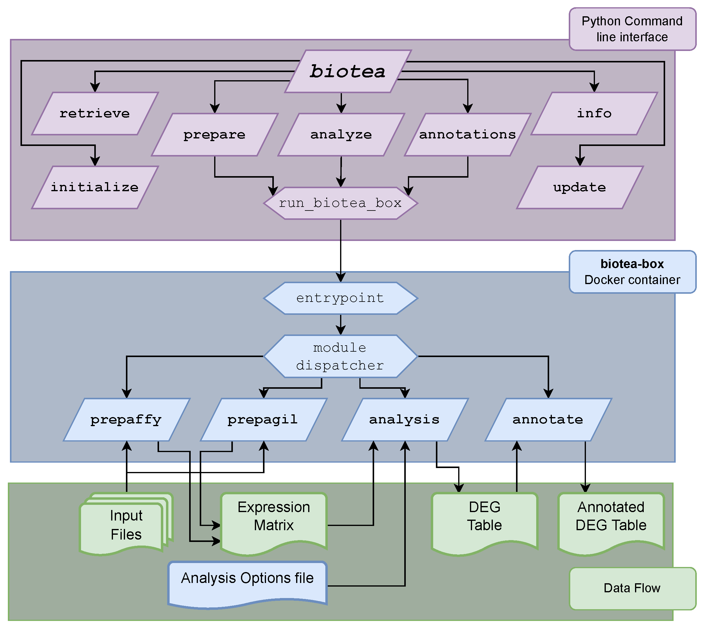
Abstract
:Simple Summary
Abstract
1. Introduction
- Despite the transcriptomics trends, thousands of articles referring to microarray experiments or microarray analyses are still published yearly [16], and this is likely to continue for a while;
- Typical pipelines for microarray analysis are custom scripts made up of multiple files and several R functions from different Bioconductor packages; dealing with this code—and correctly running a new analysis—months or years later can be source of frustration for many researchers, even among bioinformaticians.
2. Materials and Methods
- With biotea retrieve, data are directly downloaded from GEO, notably with sample metadata included that will be useful, although not required, to perform successive analysis steps.
- With biotea prepare, raw expression data (as returned by the microarray scanner setup, or as downloaded according to the previous step) are read, parsed, normalized and quality-controlled. The normalized expression matrix is saved to file, along with Quality Control (QC) plots.
- With biotea initialize, the differential expression analysis is initialized, optionally by parsing metadata about the samples. This allows the user to quickly set a variety of analysis options, such as variables of interest (e.g., treatment status), contrast of interest (e.g., “treated” vs. “control”) and analysis batches for batch effect correction. This step generates an options file that records the various choices made. This allows the user to inspect, edit or share them for reproducibility. Additional information regarding the parameters that can be set for the analysis are included in the Supplementary Methods.
- With biotea analyze, the options file (such as from the previous step) and the expression matrix are read and DEA is performed. This generates several QC plots, along with differential expression tables, as a final result. Conservative filtering is also performed on the data before the analysis, to increase statistical power.
- With biotea annotations, annotations (such as gene symbol or gene name) can be added to expression matrix files or differential expression tables to allow further analyses (such as Gene Ontology (GO) enrichment analysis) and considerations.
2.1. The bioTEA Container
2.2. Microarray Data Preparation
- Find and load all input files. prepaffy searches the target folder for all files ending with the .CEL file extension, while prepagil searches by default all .txt files. However, as .txt is a very common file extension, prepagil search criteria can be customized in the call, also supporting Regular Expressions.
- Merge all inputs into a single expression data object. Both commands do this automatically using oligo and limma packages for Affymetrix and Agilent data, respectively. From this step onward, data are expressed as values.
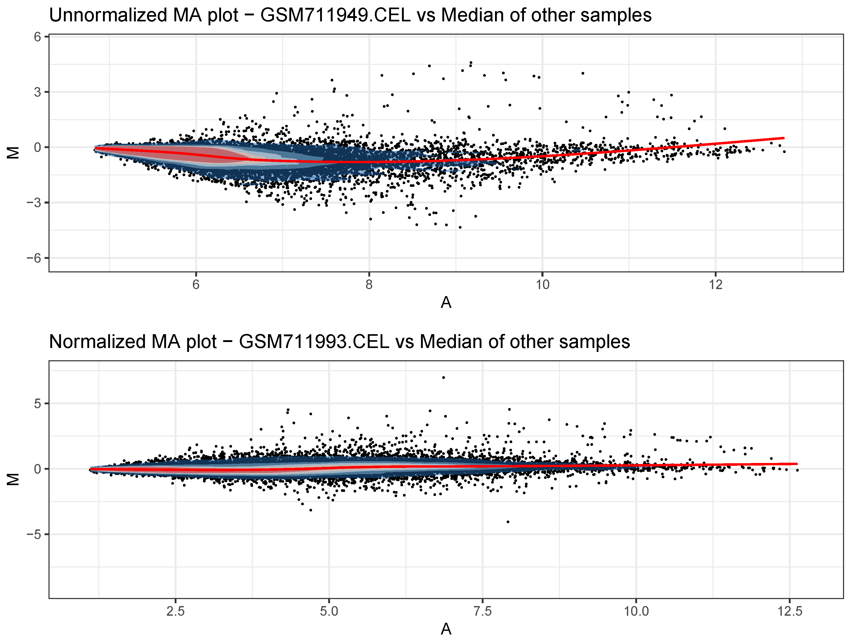
- Generate QC plots before normalization. For each sample, a Bland–Altman plot (MA plot) is saved, along with an overall expression boxplot.
- Normalize the expression data. Both data types are background-subtracted (through the normexp algorithm) and interarray-normalized (through the quantile–quantile procedure). Additionally, for Affymetrix data, the Robust Multichip Average (RMA) procedure as provided by the oligo package is used to collapse individual probes into the probe set to which they belong.
- Generate new QC plots after normalization. New MA plots and an overall expression boxplot are saved to appreciate the effects of normalization.
- If specified, remove control probes from the data set. In particular, negative control probes (i.e., sequences designed to remain unhybridized) represent a sensible estimate for the expected intensity of unexpressed genes as a result of background and nonspecific hybridization signals. Such an estimate is outputted and logged when handling Agilent data, as it can be used as a filter threshold value in the downstream analysis. This step is carried out by bioTEA for Agilent data, and by the oligo package for Affymetrix data.
- Collapse the replicate probes in Agilent arrays. Data are collapsed by taking the mean value of replicate probes found inside each sample.
- Save the final expression matrix as the output file. The expression matrix is saved in .csv format, ready to be analyzed by the other modules of bioTEA, or with customized pipelines.
2.3. Performing Differential Expression Analysis
2.4. Annotating Results
2.5. The bioTEA Command Line Interface
2.6. Source Code Availability and Installation
3. Results
3.1. Data Retrieval
3.2. Preprocessing and Quality Control
3.3. Differential Expression Analysis
4. Discussion
- Functional reproducibility ensured by Docker container technology;
- R/Bioconductor-independent CLI through Python wrapper;
- Automatic data set retrieval and metadata parsing (from GEO);
- Microarray raw data processing capability;
- Microarray multi-platform support (Agilent and Affymetrix);
- Support for RNA-seq data analysis through the voom package [28];
- Automatic annotation for many human arrays (no chip ID needed);
- Low-expression, conservative gene filtering;
- Easy experimental design definition by syntax parsing;
- Two-independent-class or paired design testing;
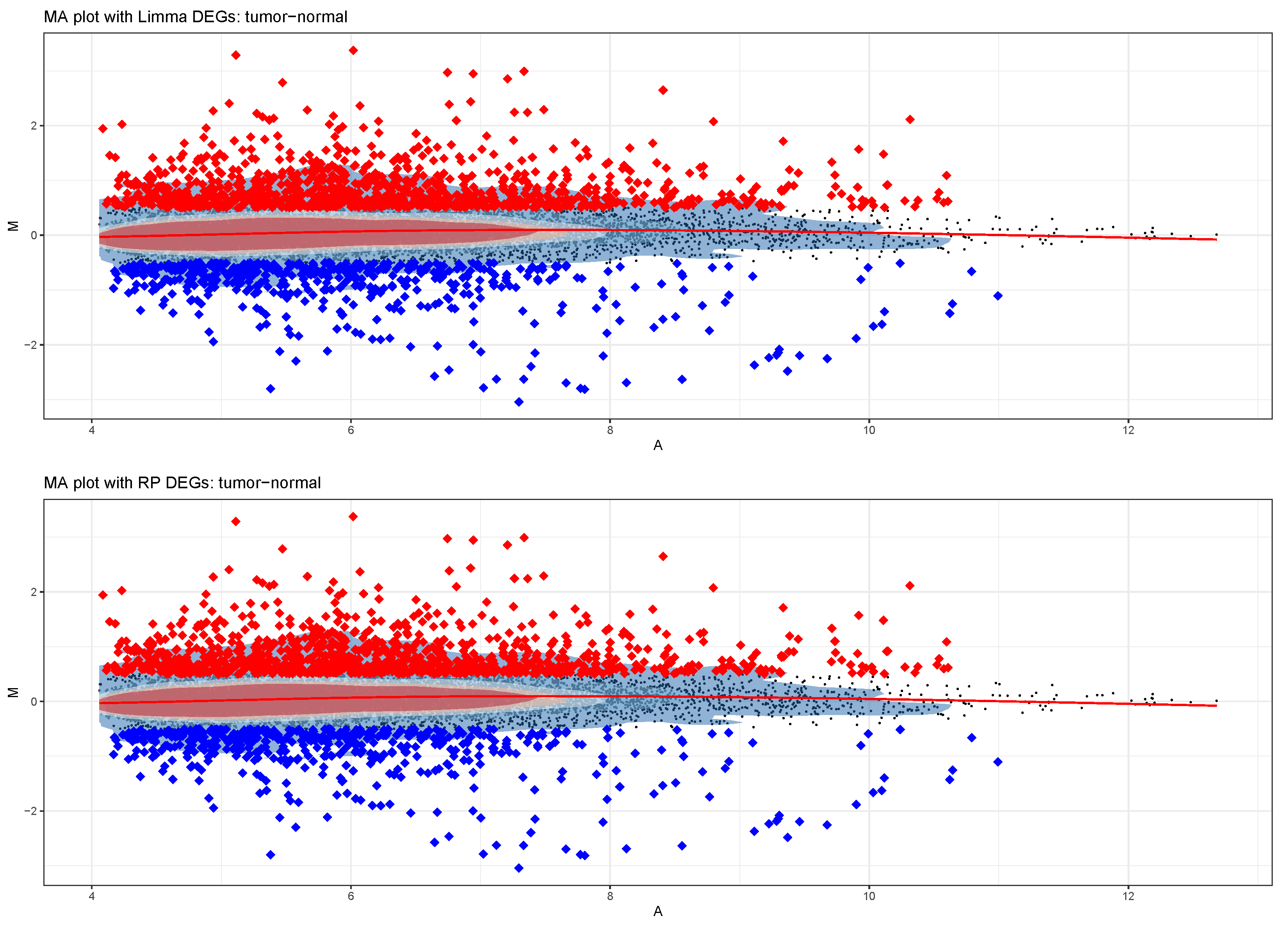
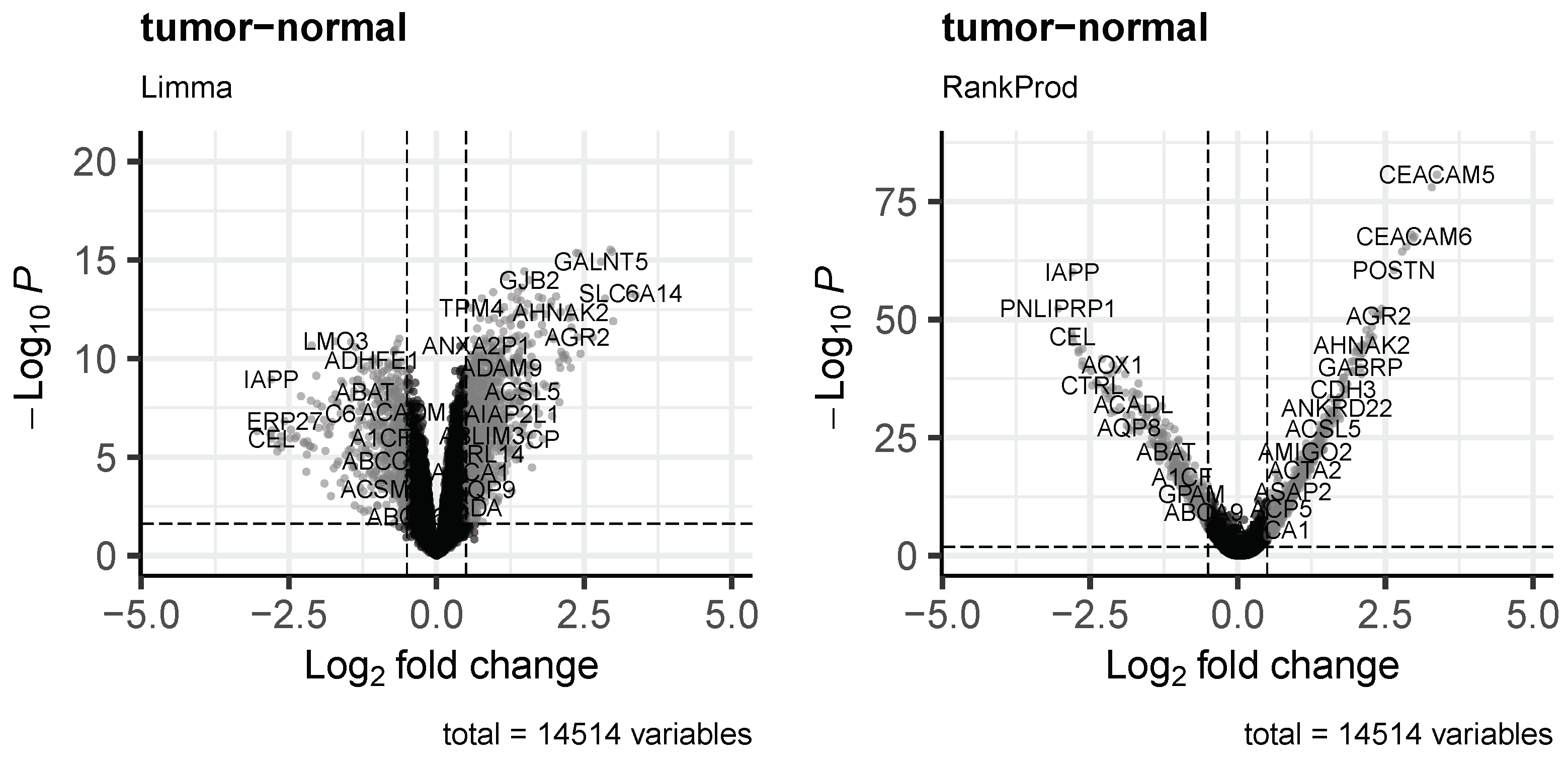
- Double approach to DEA (parametric by limma and non-parametric by RankProduct);
- Batch effect handling;
- Additional explanatory variable support;
- Detailed logging;
- High-quality graphical output;
- Detailed wiki user guide;
- Open-source and easily accessible code;
- Modular code structure suitable for further development and maintainability.
5. Conclusions
Supplementary Materials
Author Contributions
Funding
Data Availability Statement
Conflicts of Interest
Abbreviations
| AE | Array Express |
| CLI | Command Line Interface |
| DEA | Differential Expression Analysis |
| DEG | Differentially Expressed Gene |
| FDR | False Discovery Rate |
| GEO | Gene Expression Omnibus |
| GO | Gene Ontology |
| HUGO | Human Genome Organization |
| MA plot | Bland–Altman plot |
| NGS | Next-Generation Sequencing |
| PCA | Principal Component Analysis |
| PFP | Proportion of False Positives |
| QC | Quality Control |
| RMA | Robust Multichip Average |
Appendix A. Input and Output File Formats
- Expression matrix: a matrix in .csv format, with a header row, a column with entry IDs (arbitrarily named probe_id, but not necessarily representing actual probe IDs) and additional columns, one per input file, with the respective expression data (with arbitrary names). Each row in the matrix represents the expression of a single entry.
- DEG table: a matrix in .csv format, with a series of columns:
- –
- The probe_id column contains the entry IDs of the data (probe IDs or ENSEMBL IDs);
- –
- The LogFC column lists the Fold Change value of that entry, for the contrast of interest;
- –
- The AveExprs column contains the arithmetic mean of the expression values of the entry between all samples;
- –
- The t column reports the moderated t-statistic computed by limma;
- –
- The P.Value column holds the raw p-values computed by limma;
- –
- The adj.P.Val column holds the p-values computed by limma and adjusted with the Benjamini–Hochberg procedure, producing FDR values;
- –
- The B column contains the B-statistic (i.e., the empirical Bayes log-posterior odds of differential expression). Only computed by limma;
- –
- The gene.index column contains gene indexes as computed by RankProduct. Only present in the DEG table computed by RankProduct;
- –
- The RP/Rsum.UP and RP/Rsum.DOWN contain the RankProduct statistics for each entry. Only present in the DEG table computed by RankProduct;
- –
- pfp.UP and pfp.DOWN are only present in the RankProduct output. The PFP of up- and down- regulated genes, respectively;
- –
- P.Value.UP and P.Value.DOWN are only present in the RankProduct output. The p-values for up- and down- regulated genes, respectively;
- –
- The markings column marks as upregulated (1), downregulated () or non-DEG (0) each entry. For limma, this is done by the decidetests function, provided by limma, with an adjusted p-value threshold of . Additionally, genes with a lower Fold Changes than what specified by the user are marked as non differentially expressed. For RankProduct, the markings are similarly applied: genes that show a PFP value of less than are marked as up- or down- regulated (looking at the pfp.UP and pfp.DOWN values, respectively), and genes that show a fold change lower than what specified are marked as non differentially expressed.Therefore, this column can be used to quickly subset the output.
References
- Duggan, D.J.; Bittner, M.; Chen, Y.; Meltzer, P.; Trent, J.M. Expression Profiling Using cDNA Microarrays. Nat. Genet. 1999, 21, 10–14. [Google Scholar] [CrossRef] [PubMed]
- Schena, M.; Shalon, D.; Davis, R.W.; Brown, P.O. Quantitative Monitoring of Gene Expression Patterns with a Complementary DNA Microarray. Science 1995, 270, 467–470. [Google Scholar] [CrossRef] [PubMed]
- Shalon, D.; Smith, S.J.; Brown, P.O. A DNA Microarray System for Analyzing Complex DNA Samples Using Two-Color Fluorescent Probe Hybridization. Genome Res. 1996, 6, 639–645. [Google Scholar] [CrossRef] [PubMed]
- Larkin, J.E.; Frank, B.C.; Gavras, H.; Sultana, R.; Quackenbush, J. Independence and Reproducibility across Microarray Platforms. Nat. Methods 2005, 2, 337–344. [Google Scholar] [CrossRef] [PubMed]
- Tarca, A.L.; Romero, R.; Draghici, S. Analysis of Microarray Experiments of Gene Expression Profiling. Am. J. Obstet. Gynecol. 2006, 195, 373–388. [Google Scholar] [CrossRef]
- Mayo, M.S.; Gajewski, B.J.; Morris, J.S. Some Statistical Issues in Microarray Gene Expression Data. Radiat. Res. 2006, 165, 745–748. [Google Scholar] [CrossRef]
- Verducci, J.S.; Melfi, V.F.; Lin, S.; Wang, Z.; Roy, S.; Sen, C.K. Microarray Analysis of Gene Expression: Considerations in Data Mining and Statistical Treatment. Physiol. Genom. 2006, 25, 355–363. [Google Scholar] [CrossRef]
- Slonim, D.K.; Yanai, I. Getting Started in Gene Expression Microarray Analysis. PLoS Comput. Biol. 2009, 5, e1000543. [Google Scholar] [CrossRef]
- Chen, J.J. Key Aspects of Analyzing Microarray Gene-Expression Data. Pharmacogenomics 2007, 8, 473–482. [Google Scholar] [CrossRef]
- Gentleman, R.C.; Carey, V.J.; Bates, D.M.; Bolstad, B.; Dettling, M.; Dudoit, S.; Ellis, B.; Gautier, L.; Ge, Y.; Gentry, J.; et al. Bioconductor: Open Software Development for Computational Biology and Bioinformatics. Genome Biol. 2004, 5, R80. [Google Scholar] [CrossRef] [Green Version]
- Home-GEO-NCBI. Available online: https://www.ncbi.nlm.nih.gov/geo/ (accessed on 25 July 2022).
- Edgar, R.; Domrachev, M.; Lash, A.E. Gene Expression Omnibus: NCBI Gene Expression and Hybridization Array Data Repository. Nucleic Acids Res. 2002, 30, 207–210. [Google Scholar] [CrossRef] [PubMed]
- Browse < ArrayExpress < EMBL-EBI. Available online: https://www.ebi.ac.uk/arrayexpress/browse.html (accessed on 25 July 2022).
- Brazma, A.; Parkinson, H.; Sarkans, U.; Shojatalab, M.; Vilo, J.; Abeygunawardena, N.; Holloway, E.; Kapushesky, M.; Kemmeren, P.; Lara, G.G.; et al. ArrayExpress–a Public Repository for Microarray Gene Expression Data at the EBI. Nucleic Acids Res. 2003, 31, 68–71. [Google Scholar] [CrossRef] [PubMed]
- Wang, Z.; Gerstein, M.; Snyder, M. RNA-Seq: A Revolutionary Tool for Transcriptomics. Nat. Rev. Genet. 2009, 10, 57–63. [Google Scholar] [CrossRef] [PubMed]
- Lowe, R.; Shirley, N.; Bleackley, M.; Dolan, S.; Shafee, T. Transcriptomics Technologies. PLoS Comput. Biol. 2017, 13, e1005457. [Google Scholar] [CrossRef]
- Sabaie, H.; Mazaheri Moghaddam, M.; Mazaheri Moghaddam, M.; Amirinejad, N.; Asadi, M.R.; Daneshmandpour, Y.; Hussen, B.M.; Taheri, M.; Rezazadeh, M. Long Non-Coding RNA-associated Competing Endogenous RNA Axes in the Olfactory Epithelium in Schizophrenia: A Bioinformatics Analysis. Sci. Rep. 2021, 11, 24497. [Google Scholar] [CrossRef]
- Leal-Calvo, T.; Moraes, M.O. Reanalysis and Integration of Public Microarray Datasets Reveals Novel Host Genes Modulated in Leprosy. Mol. Genet. Genom. MGG 2020, 295, 1355–1368. [Google Scholar] [CrossRef]
- Baker, M. 1500 Scientists Lift the Lid on Reproducibility. Nature 2016, 533, 452–454. [Google Scholar] [CrossRef]
- Begley, C.G.; Ellis, L.M. Drug Development: Raise Standards for Preclinical Cancer Research. Nature 2012, 483, 531–533. [Google Scholar] [CrossRef]
- Samsa, G.; Samsa, L. A Guide to Reproducibility in Preclinical Research. Acad. Med. J. Assoc. Am. Med Coll. 2019, 94, 47–52. [Google Scholar] [CrossRef]
- Sandve, G.K.; Nekrutenko, A.; Taylor, J.; Hovig, E. Ten Simple Rules for Reproducible Computational Research. PLoS Comput. Biol. 2013, 9, e1003285. [Google Scholar] [CrossRef] [Green Version]
- Ritchie, M.E.; Phipson, B.; Wu, D.; Hu, Y.; Law, C.W.; Shi, W.; Smyth, G.K. Limma Powers Differential Expression Analyses for RNA-sequencing and Microarray Studies. Nucleic Acids Res. 2015, 43, e47. [Google Scholar] [CrossRef] [PubMed]
- Hong, F.; Breitling, R.; McEntee, C.W.; Wittner, B.S.; Nemhauser, J.L.; Chory, J. RankProd: A Bioconductor Package for Detecting Differentially Expressed Genes in Meta-Analysis. Bioinformatics 2006, 22, 2825–2827. [Google Scholar] [CrossRef] [PubMed]
- Del Carratore, F.; Jankevics, A.; Eisinga, R.; Heskes, T.; Hong, F.; Breitling, R. RankProd 2.0: A Refactored Bioconductor Package for Detecting Differentially Expressed Features in Molecular Profiling Datasets. Bioinformatics 2017, 33, 2774–2775. [Google Scholar] [CrossRef] [PubMed]
- Nygaard, V.; Rødland, E.A.; Hovig, E. Methods That Remove Batch Effects While Retaining Group Differences May Lead to Exaggerated Confidence in Downstream Analyses. Biostatistics 2016, 17, 29–39. [Google Scholar] [CrossRef] [PubMed]
- Putri, G.H.; Anders, S.; Pyl, P.T.; Pimanda, J.E.; Zanini, F. Analysing High-Throughput Sequencing Data in Python with HTSeq 2.0. Bioinformatics 2022, btac166. [Google Scholar] [CrossRef]
- Law, C.W.; Chen, Y.; Shi, W.; Smyth, G.K. Voom: Precision Weights Unlock Linear Model Analysis Tools for RNA-seq Read Counts. Genome Biol. 2014, 15, R29. [Google Scholar] [CrossRef]
- bioTEA · PyPI. Available online: https://pypi.org/project/bioTEA/ (accessed on 25 July 2022).
- BioTEA. CMA-Lab. 2022. Available online: https://github.com/CMA-Lab/bioTEA (accessed on 25 July 2022).
- Cmalabscience/Biotea-Box Tags | Docker Hub. Available online: https://hub.docker.com/r/cmalabscience/biotea-box/tags (accessed on 25 July 2022).
- Preston-Werner, T. Semantic Versioning 2.0.0. Available online: https://semver.org/ (accessed on 25 July 2022).
- Zhang, G.; Schetter, A.; He, P.; Funamizu, N.; Gaedcke, J.; Ghadimi, B.M.; Ried, T.; Hassan, R.; Yfantis, H.G.; Lee, D.H.; et al. DPEP1 Inhibits Tumor Cell Invasiveness, Enhances Chemosensitivity and Predicts Clinical Outcome in Pancreatic Ductal Adenocarcinoma. PLoS ONE 2012, 7, e31507. [Google Scholar] [CrossRef]
- Zhang, G.; He, P.; Tan, H.; Budhu, A.; Gaedcke, J.; Ghadimi, B.M.; Ried, T.; Yfantis, H.G.; Lee, D.H.; Maitra, A.; et al. Integration of Metabolomics and Transcriptomics Revealed a Fatty Acid Network Exerting Growth Inhibitory Effects in Human Pancreatic Cancer. Clin. Cancer Res. Off. J. Am. Assoc. Cancer Res. 2013, 19, 4983–4993. [Google Scholar] [CrossRef]
- Barrett, T.; Wilhite, S.E.; Ledoux, P.; Evangelista, C.; Kim, I.F.; Tomashevsky, M.; Marshall, K.A.; Phillippy, K.H.; Sherman, P.M.; Holko, M.; et al. NCBI GEO: Archive for functional genomics data sets–update. Nucleic Acids Res. 2013, 41, D991–D995. [Google Scholar] [CrossRef]
- Amaral, M.L.; Erikson, G.A.; Shokhirev, M.N. BART: Bioinformatics array research tool. BMC Bioinform. 2018, 19, 296. [Google Scholar] [CrossRef] [Green Version]
- Howe, E.A.; Sinha, R.; Schlauch, D.; Quackenbush, J. RNA-Seq analysis in MeV. Bioinformatics 2011, 27, 3209–3210. [Google Scholar] [CrossRef] [PubMed] [Green Version]


Publisher’s Note: MDPI stays neutral with regard to jurisdictional claims in published maps and institutional affiliations. |
© 2022 by the authors. Licensee MDPI, Basel, Switzerland. This article is an open access article distributed under the terms and conditions of the Creative Commons Attribution (CC BY) license (https://creativecommons.org/licenses/by/4.0/).
Share and Cite
Visentin, L.; Scarpellino, G.; Chinigò, G.; Munaron, L.; Ruffinatti, F.A. BioTEA: Containerized Methods of Analysis for Microarray-Based Transcriptomics Data. Biology 2022, 11, 1346. https://doi.org/10.3390/biology11091346
Visentin L, Scarpellino G, Chinigò G, Munaron L, Ruffinatti FA. BioTEA: Containerized Methods of Analysis for Microarray-Based Transcriptomics Data. Biology. 2022; 11(9):1346. https://doi.org/10.3390/biology11091346
Chicago/Turabian StyleVisentin, Luca, Giorgia Scarpellino, Giorgia Chinigò, Luca Munaron, and Federico Alessandro Ruffinatti. 2022. "BioTEA: Containerized Methods of Analysis for Microarray-Based Transcriptomics Data" Biology 11, no. 9: 1346. https://doi.org/10.3390/biology11091346