1. Introduction
Human gait can be considered a quasiperiodic phenomenon. Despite the apparent stability of walking at a constant speed, gait exhibits an inherent local variability that can be observed at the level of basic parameters such as the stride-to-stride interval time, or simply referred to as the stride interval (SI). The global stability during gait is typically assessed by quantifying the whole-body center-of-mass (COM) motion. Local variability can be modulated to maintain global stability [
1].
It is well known that gait variability is a hallmark of healthy individuals and has properties that are far more complex than stochastic variability. Since the seminal works of Haussdorff et al. [
2,
3], it has been shown that the variability, more exactly the predictability, of SI over a long period of time—typically several hundred gait cycles—is autocorrelated, just as it is in chaotic systems. These autocorrelations can be assessed by computing the Hurst exponent or H [
4,
5], which typically ranges from 0.7 to 0.9 in young healthy adults [
6]. Note that H = 0.5 implies random variability. Although the physiological mechanism that generates SI autocorrelations is still controversial, neurodegenerative diseases significantly alter SI variability [
7], and the use of indices other than H can help distinguish between different pathologies [
8,
9]. Other disturbances during walking, such as the execution of a cognitive task [
10] or following a rhythmic auditory cue [
11], also alter SI variability.
Realistic values for H can be obtained by resorting to simple mechanical models of the inverted pendulum type, in which one or two parameters are randomly updated at the beginning of each step [
12,
13]. Although mechanical approaches are used to model gait variability, it is worth noting that developments in Mechanics, such as action-angle variables in the Hamiltonian formalism, have proven to be remarkably successful in finding conserved quantities for complex and even chaotic systems [
14,
15], i.e., quantities with invariant value over time. Identifying such a conserved quantity for human gait would be to find dynamical constraints “hiding” behind SI variability that could provide new insights into how dynamical systems, in which behaviors evolve over time, maintain their current state or stability while allowing for variability/predictability. Whereas energy is not necessarily conserved over time with stochastic variation in system parameters, adiabatic invariants are good candidates for (almost) conserved quantities. An adiabatic invariant,
I, is a quantity that remains approximately constant during the evolution of a dynamical system even under slow external changes, i.e., an adiabatic transformation [
14]. One way to define an adiabatic invariant, I, relevant to the analysis of rhythmic human motion for a given degree of freedom
for which the kinetic energy has the standard form
[
16], with
m a mass scale, is through
where
,
f is a given cycle frequency (the inverse of its duration) and
is the averaged kinetic energy on the cycle under consideration. In the model (Equation (
1)),
and
f are assumed to change significantly over time, but their ratio, which is proportional to
I, should remain invariant. Here,
during each gait cycle will be computed from the whole-body COM vertical displacement. The term “adiabatic invariant” will therefore refer to the quantity (
1) computed from the vertical displacement of the COM. It is an important restriction, since in principle, adiabatic invariants may be found in the other directions and for other degrees of freedom while walking. Another important remark is the following. The term “invariant” will be used to denote a function of the dynamical variables whose value does not change over time during the evolution of a dynamical system, while the word “constant” will be used for a parameter whose value is not modified by the experimental condition. A textbook example is that of a simple pendulum without friction: Total energy is invariant but not constant, since it depends on the amplitude.
Biological systems are the most noteworthy nonconservative systems that derive forces from internal energy reservoirs [
17]. In previous work, the adiabatic invariant has been successfully applied to human movement [
17]. In biological systems, it is also important to note that adiabatic invariants can be considered only as an approximation and are not rigorously but rather approximately invariant.
Previous work has shown that the relations (
1) holds for rhythmic arm movements [
17,
18] and for walking [
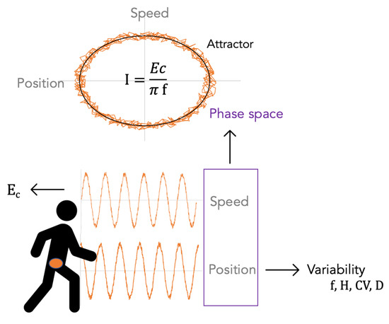
19]. In the latter work, participants walked for 3 min, and SI variability was not examined. More, limit cycle attractors in phase space
, i.e., the average gait cycle of a participant, were not drawn while they can also be used as a visual representation of gait pattern. Human motion, and particularly walking, is indeed highly stereotyped, though noisy, and gait patterns are highly consistent for an individual over time [
20]. The attractors may also distinguish between walking and running, as the transition from walking to running can be viewed as a change from one stable attractor to another [
21]. Therefore, these attractors could help distinguish between participants and conditions. The area enclosed by the phase-space trajectory of system over one cycle is the adiabatic invariant
I.
From the perspective of understanding the role played by the neuro-musculoskeletal system in constraining coordination and reducing the degrees of freedom [
22], adiabatic invariants of motion are relevant quantities, since two or more variables are linked by a single invariant. Therefore, the primary objective of this study is to investigate whether the adiabatic invariant model (
1) holds in a population of healthy young adults walking at spontaneous speed on a motorized treadmill during a sufficient number (typically more than 500) of cycles to also assess SI variability, predictability, and complexity. The secondary objective is to understand how a constraint applied on the system, in our case, a rhythmic auditory cue (metronome) indicating preferred step frequency, impact global stability (assessed using the adiabatic invariant
I) and SI variables. Our hypotheses were that Equation (
1) holds during walking on a treadmill, regardless of the metronome constraint, and that the latter constraint exhibits significant variability and predictability indices, as shown in [
11].
2. Materials and Methods
2.1. Protocol
The protocol was performed in a session of approximately 60 min. It was validated by the Academic Ethical Committee Brussels Alliance for Research and Higher Education (protocol B200-2021-123). Participants were healthy students recruited in the Department of Physiotherapy of the Haute Ecole Louvain en Hainaut (Montignies-sur-Sambre, Belgium). After being informed of the study, each participant signed an informed consent. The same experimenters (F.P. and G.H.) were responsible for the measurements.
First, participants’ age and biometric data (mass and height) were collected. Participants were asked to wear a tight outfit. Participants’ pelvic movements were recorded using a Vicon opto-electronic system (Vicon Motion Systems Ltd, Oxford Metrics, Oxford, UK) composed of 8 cameras (Vero v.2.2) with a sampling frequency of 120 Hz. Four 14 mm diameter reflective markers were placed on the pelvis of the participants following the Plug-In-Gait model (Oxford Metrics, Oxford, UK): Left Anterior Superior Iliac Spine (LASI), Right Anterior Superior Iliac Spine (RASI), Left Posterior Superior Iliac Spine (LPSI), and Left Posterior Superior Iliac Spine (RPSI).
Then, participants took place on the belt of an instrumented motorized treadmill (N-Mill, Motekforce Link, The Netherlands). The vertical ground reaction force and center of pressure of each foot was recorded at a sampling rate of 500 Hz using the manufacturer’s software (CueFors 2, Motekforce Link, The Netherlands). Spontaneous walking speed was determined and recorded during a 3-minute habituation period. After a 1-minute rest, the participant walked at a spontaneous speed on the treadmill for 10 min (control condition, CTRL). The average step frequency, f, was automatically computed by the CueFors 2 software. The positions of the 4 markers, , were recorded with the Vicon system via the Vicon Nexus software (v.2.7.1, Oxford Metrics, Oxford, UK). After a short break of 3 min, the participant walked on the treadmill at a spontaneous speed for 10 min with instructions to synchronize his or her steps with the clicks of a metronome whose tempo corresponded to the number of steps per minute calculated in the CTRL condition (metronome condition, METRO). This allowed the participants to adjust their gait tempo on a step basis whilst ensuring they adopted their own comfortable pace. The duration of the successive gait cycles and the positions of the 4 markers were recorded in the METRO condition.
To estimate the whole-body COM vertical trajectory,
, the mean vertical position of all pelvic markers (RASI, LASI, LPSI, and RPSI) was taken at each time step. Furthermore, to reduce measurement artefacts,
was filtered using a low-pass fourth-order Butterworth filter adjusted to each time series so that it kept 99.99% of the signal’s power. In order to alleviate the low sampling rate of the measurement system, a cubic spline interpolation was conducted on the data, multiplying the frequency by 10 to 1200 Hz. The speed and acceleration were then obtained through a finite difference scheme. The data was processed using R software (v. 4.1.0) [
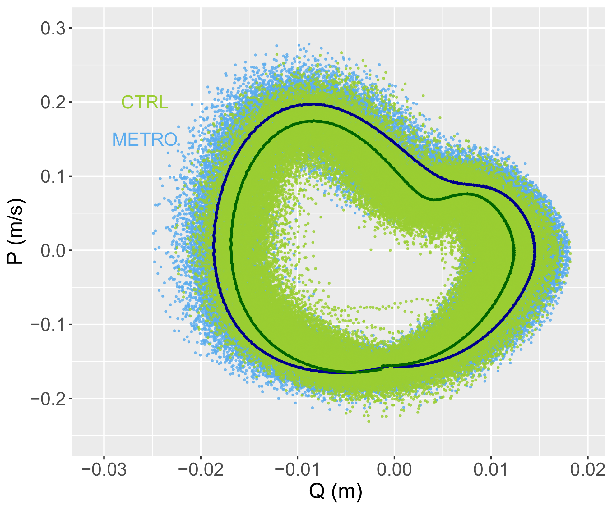
23]. Typical phase-space trajectories are shown in
Figure 1.
2.2. Adiabatic Invariant I (Global Stability)
We assume that the vertical motion of the whole-body COM during walking is governed by the Hamiltonian
, with
and
a stochastic noise. This model is based on a forced harmonic oscillator with a frequency that fluctuates randomly around a mean
. The noise accounts for physiological noise (i.e., the impossibility for the human locomotor system to be steadily in the same state) and should be low in healthy individuals. The momentum
P is defined as
, as in standard Hamiltonian mechanics. This general class of Hamiltonians fits the form considered in the
Appendix A, where the computational details are given. As developed in this
Appendix A, the action variable (
1) is an adiabatic invariant of the system: its value does not change over time except for small random fluctuations around the mean. In summary, the linear relationship (
1) is to be expected in the analysis of the vertical motion of COM in healthy walking individuals.
A step is defined by the collection of data points between two maxima in
. A gait cycle consists of two consecutive steps. For each gait cycle identified, denoted
, the frequencies
and the average kinetic energy
were computed. Recall that
i typically ranges from 1 to 500. For a given participant in a given condition, we computed
,
, and
, where
denotes the arithmetic mean of an arbitrary set of values
. Equation (
1) is valid for all values of
, and we assume that
I is constant according to adiabatic invariant theory [
14]. Taking into account Equation (
1) together with
leads to
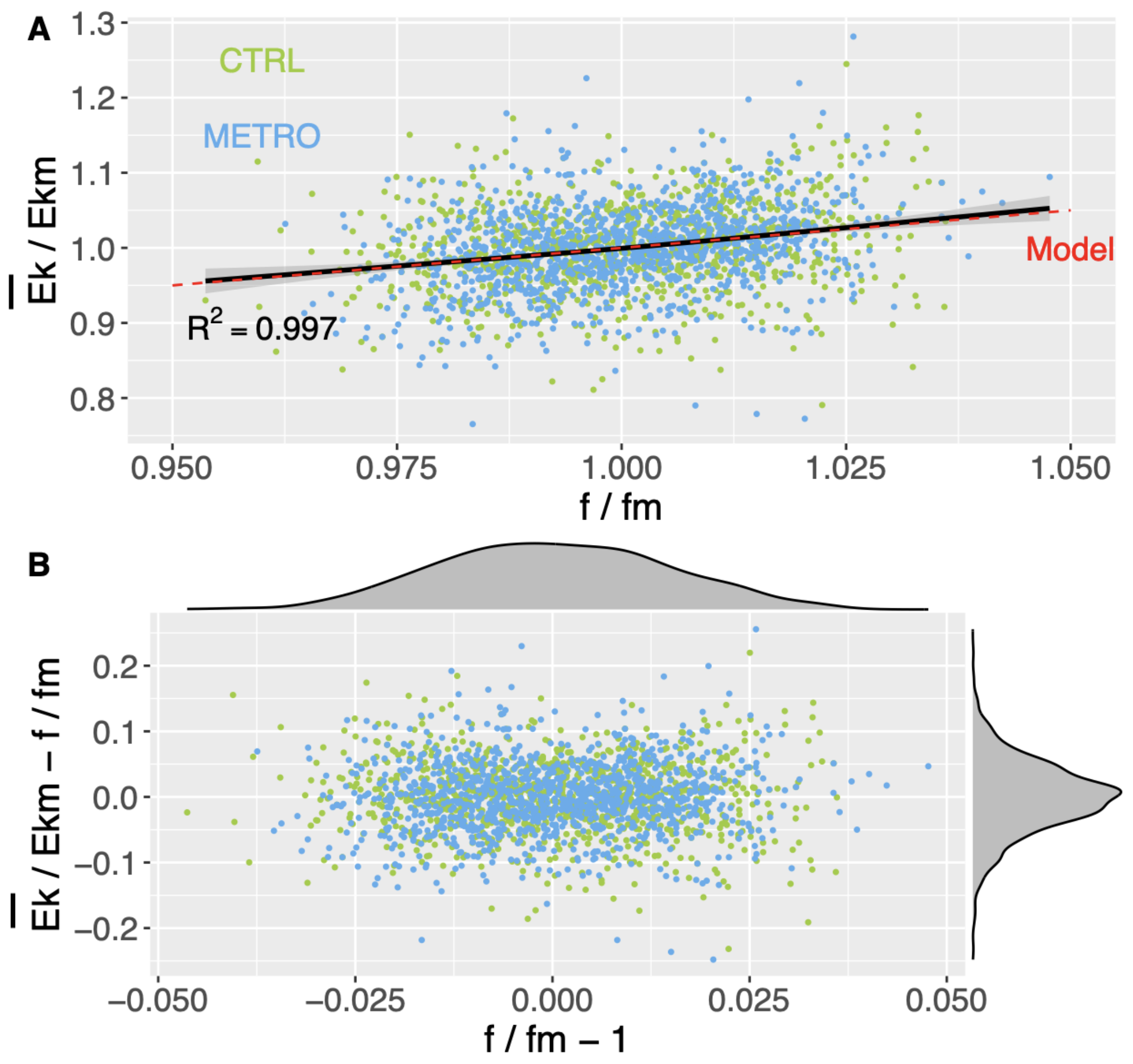
Therefore, a prediction of our model is that versus should behave as a straight line with slope 1 and a zero intercept.
After each gait cycle was identified, an average cycle was computed. To do this, each cycle was normalized to a unit duration and a spline of 1200 equally spaced points was computed for each cycle. Then, 1200 bins—one for each frame—were created and filled with the data from the splines of all cycles of a given participant in a given condition. The mean and standard deviation were computed for each bin.
2.3. SI Variability, Predictability, and Complexity
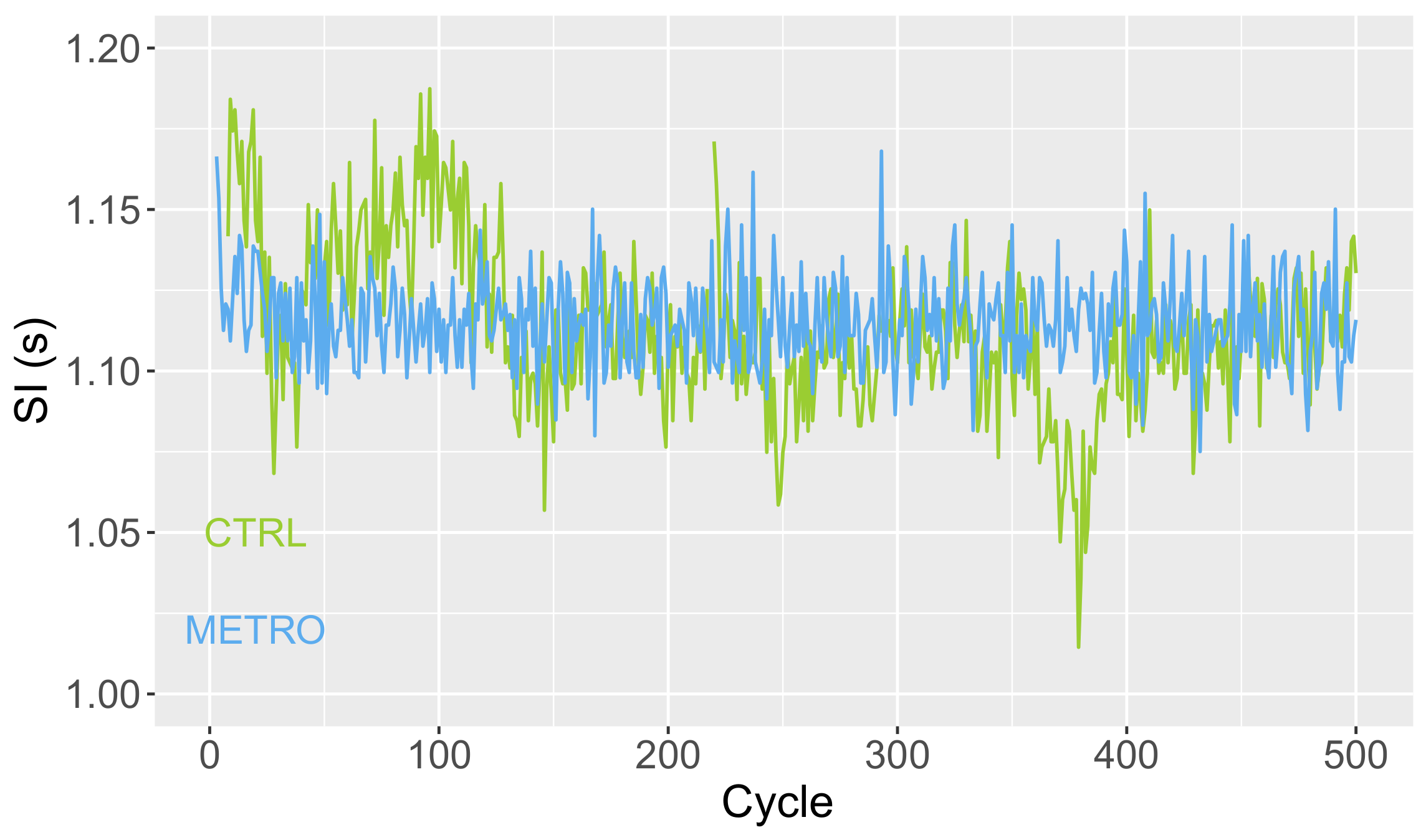
Time series
with durations
of successive gait cycles were computed from heel strikes of the right foot identified by CueFors 2 software. At the end of the session, two time series were generated for each subject in the CTRL and METRO conditions. Typical plots are shown in
Figure 2.
First, the average SI was computed, as well as the coefficient of variation, CV =
, estimating the magnitude of SI fluctuations. The Hurst exponent, H, was then computed by resorting to Detrended Fluctuation Analysis following the guidelines in [
6]; more technical details about the algorithm we used can be found in [
24]. By definition,
H is mainly a measure of the time series’ predictability [
4,
5]. Therefore, it is relevant to complement it with other variability indices [
8,
9,
25], of which we have chosen the Minkowski fractal dimension, D, [
24], and the sample entropy, S, both as measures of complexity [
1]. Computational details for D can be found in [
24], while S was computed using the method described in [
26]. All SI data analysis was performed with R (v. 4.1.0).
Figure 2 gives a first hint of SI variability, predictability, and complexity. Fluctuations around the mean value have a smaller magnitude in the METRO condition (smaller CV), but a simpler temporal structure. Indeed, the latter fluctuations show increasing or decreasing trends during several tenths of cycles in CTRL conditions, resulting in a larger predictability (larger H). The lower predictability in the METRO condition also results in a larger sample entropy, meaning that the fluctuations are closer to a random process in the METRO condition. Indeed, S is maximal for a random process.
As discussed in
Appendix A, CV provides an estimate of
, the magnitude of the time-dependent noise modeling the quasiperiodic nature of human motion. As our approach is only valid for
well smaller than 1, the measured values of CV must be well smaller than 1 too, for our approach to be consistent.
2.4. Statistical Analysis
Data assessing SI variability, predictability, and complexity were tested for normality (Shapiro–Wilk) and equality of variance test. A paired t-test was performed and used to examine the effects of condition (CTRL or METRO) on SI, CV, H, D, and S. The significance level was set at . In the case of a failed normality test, a Wilcoxon signed rank test was performed. The adiabatic invariant I was compared in the CTRL and METRO conditions using the same methodology. All these statistical procedures were performed with SigmaPlot software version 11.0 (Systat Software, San Jose, CA, USA).
An ANCOVA with zero intercept and significance level
was performed to compare the linear trends of
versus
in conditions CTRL and METRO, i.e., according to model
where
k is the experimentally observed slope. A linear regression with zero intercept of
versus
was also performed independently of the condition, and the 95% confidence interval of the slope was computed. ANCOVA was performed with R software (v. 4.1.0).
Dynamic Time Warping (DTW), an algorithm developed to measure “distances” between similarly patterned time series, was then run to compare the distance between CTRL and METRO conditions for each participant whole-body COM vertical position (Q) and speed (P) as a function of time. The distances were computed for Q and compared to that computed for P using a paired t-test. The `dtw’ package in R was used, and the time series were z-normalized before comparison between the time series.
4. Discussion
The objectives of this study were twofold: (1) to investigate whether the adiabatic invariant model (Equation (
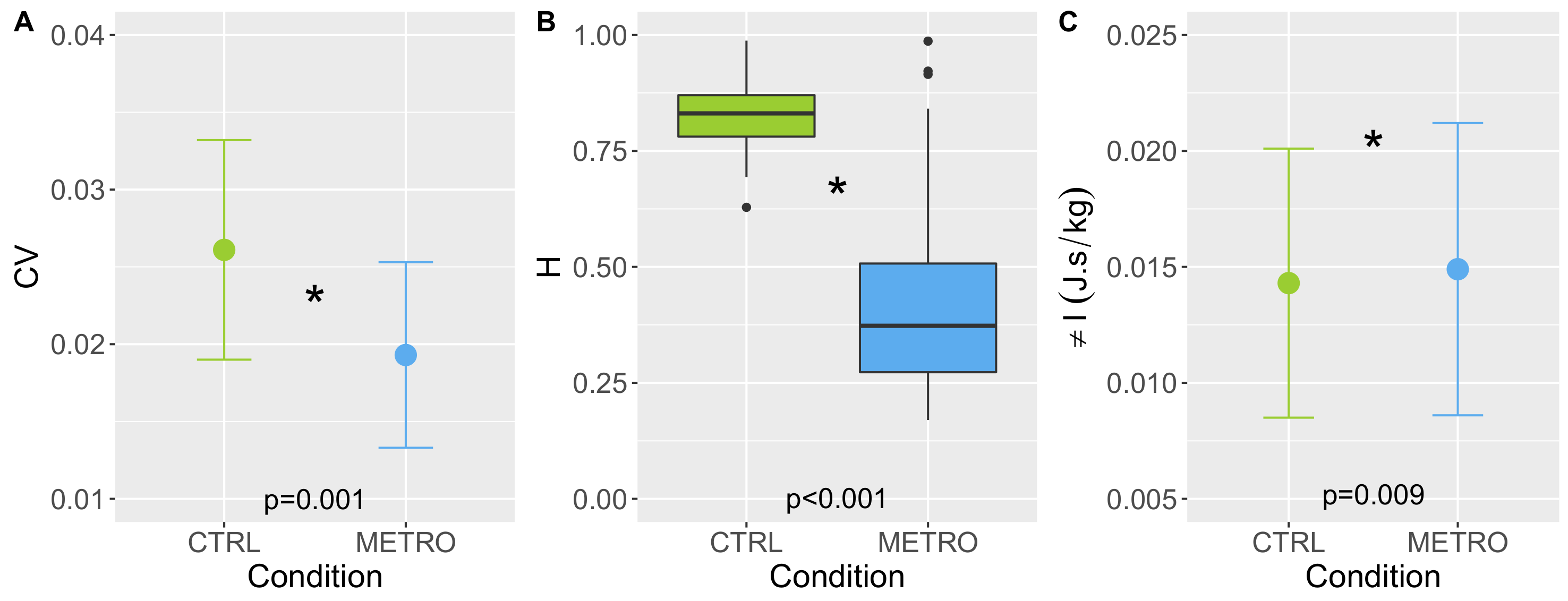
1)) holds in a population of healthy young adults walking at spontaneous speed on a motorized treadmill, and (2) to understand how a constraint applies on the system with a metronome impact global stability and SI variables. The major findings were that: (1) the invariant model was verified, and (2) SI variabilty (CV) and predictability (H) significantly decreased in the METRO condition, and global stability (
I) significantly increased in the METRO condition.
The originality of this work is that it simultaneously measured the global stability, and local variability, predictability, and complexity of motorized-treadmill walking in two conditions. In the first, CTRL, participants walked at spontaneous speed. In the second, METRO, participants adjusted heel strikes to a tone emitted by a metronome whose frequency matched each participant’s preferred frequency. The latter condition is known to induce significant changes in step-to-step variation [
11], and this was also the case in our study. We first comment on the SI variability, predictability, and complexity results. The values we found are typical of the long-range variability observed in healthy young adults; see, e.g., [
9,
24] for CV, H, and D, and [
25] for S. A salient feature of our results is the decrease in H from correlated (H = 0.848) to anti-correlated (H = 0.373) values. This phenomenon was previously observed in [
11]. The metronome that clicks at the spontaneous frequency of a participant “destroys” the normal SI autocorrelation pattern [
11]. This can be interpreted by the additional constraint that the metronome imposes. Here, the participant is not free to adapt his/her variability, as would be the case with an optimal motor strategy, but must inhibit any change in SI variability to remain synchronous with the metronome. This blocking mechanism leads to anti-correlation, and also to a much smaller CV in the METRO condition. Note that CV is much smaller than 1 in both conditions, and so it is consistent with our mechanical approach, where the magnitude of the time-dependent noise is assumed to be small. S is almost significantly higher in the METRO condition. This could be related to the fact that the q3 value of H in METRO condition is equal to 0.56: a non-negligible fraction of our participants has H around 0.5, and random variability has maximum entropy.
Our major observation is that the model (
3) holds in both the CTRL and METRO conditions. Although the participants change their SI variability and predictability, the dynamical stability constraint induced by the adiabatic invariance is verified:
of the whole-body COM and
f of a given cycle are linearly correlated. Note that the model (
3) does not forbid changing the value of
I in the different conditions. By the way, the adiabatic invariant
I is significantly higher in the condition METRO. On the one hand,
. On the other hand,
f does not change significantly in the METRO condition because
T does not change. Thus, the increase in
I is associated with a higher
per gait cycle. Regarding phase-space dynamics, the DTW distance for
P is not significantly different from that for
Q. This result does not allow us to infer that the change in
I is mostly due to a change of behavior in one of the variables
P or
Q. Instead, it shows that the change in
I is due to a simultaneous change of both
P and
Q behaviors.
Strategies for human locomotion based on adiabatic invariance have already been developed and computed from the total (translational and rotational) body’s kinetic energy per stride [
19]. In this study, a multi-segmental model was used, in which the body segments were treated as an ensemble of systems in motion, each characterized within a stride by the summed changes in kinetic energies from and about their respective centers-of-mass. In this model, walking is viewed as a sequence of joint rotations, and is referred to as a “segmental” approach [
27]. Here, we extend the results of this previous work, as we were able to show the validity of the theory of adiabatic invariance in walking using a single-point kinematic model represented by the vertical component of the whole-body COM. The latter is known to provide summarized information about all body segments during walking. In contrast to the previous model, walking is considered as achieving a forward motion of the whole-body system [
27]. Even more interesting is that the vertical displacement of the whole-body COM is related to the metabolic cost [
28]. Therefore, we hypothesize that
I is related to the metabolic cost of walking, and that participants are able to follow the metronome constraint at the expense of a larger oxygen consumption (
). This picture is coherent with [
29], in which it is shown that an altered SI variability correlates with higher
. However, the changes in variability in the latter study were due to different walking speeds, which are not comparable with our protocol. It has also been shown that the nervous system uses predictions of the optimal gait to optimize the energetic cost of each new step [
30]. This has also been demonstrated in other activities such as pedalling [
31]. We think that keeping a constant value for
I during walk with a given set of external conditions is one of the constraints involved in the prediction of the nervous system. The presence of such a constraint may actually improve the efficiency of prediction by excluding irrelevant motor strategies and reducing the degrees of freedom of the neuro-musculoskeletal system [
22].
From a methodological viewpoint, we choose to compute
of the whole-body COM only in the vertical direction (sagittal plane motion), and not in the anteroposterior and mediolateral directions (horizontal and transverse plane motion). This choice could be justified by the methodology implemented for SI variables assessment requiring numerous gait cycles. Walking on a motorized treadmill is not similar to walking on the ground, and station-keeping on the belt is impossible and surely less important than not falling [
32]. Displacement of the whole-body COM in the horizontal and transverse planes is mainly related to foot placement dynamics on the belt that may be affected to the motion strategy adopted by the participants; for example, if they want to avoid the belt’s edge [
32]. Therefore, the displacement of the COM in horizontal and transverse planes was excluded from our analyses, since the motion in this plane is not representative of a spontaneous motion from a walk on the ground. Moreover, a drift correction method should have been considered before calculating the adiabatic invariants, which is out of the scope of our paper. As a consequence, only one adiabatic invariant has been computed, while from the separability hypothesis, three adiabatic invariants should be possibly computed from the COM motion during walk, one per direction. Further studies are now necessary to explore this statement.
The present study has some limitations that should be addressed. First, we considered the CTRL condition as a reference to compare the effects of the metronome. However, walking on a motorized treadmill results in an anti-correlated pattern in the stride speed fluctuations [
11]. Therefore, the best reference condition is walking on the ground, but recording the kinematics of the pelvis during a large number of cycles is not possible without moving to half-turns in the calibrated volume, which would lead to a disturbance of the locomotor rhythm. Second,
was not measured during walking. However, a direct relationship between total body kinetic energy and
was previously observed at various constant walking speeds [
19]. The measurement of
would have allowed us to test our hypothesis formulated above regarding the relationship between
I and the metabolic cost of walking. Third, we use a reduced kinematic pelvic model with four markers to estimate the whole-body COM position instead of a whole-body kinematic model. However, we believe that our pelvic model is more robust than the single sacral marker method, which is a too rough approximation of COM, given that the latter can move with respect to the sacrum [
27]. The pelvic model is also theoretically controlled for pelvic tilt motion [
33], and assumes that the pelvis position could be an approximation of the whole-body COM position [
32]. More, the pelvic model is favored by clinicians during routine gait analysis to reduce the experimental and postprocessing times. Therefore, we hope that the reduced kinematic pelvic model used here will be an incentive to test the existence of global stability of the whole-body COM in pathological populations.
In summary, we have shown for the first time that an adiabatic invariant,
I (see Equation (
1)), is a robust dynamical stability constraint on SI variability and predictability. In other words, the vertical speeds and positions of one individual’s COM during successive walking cycles are not arbitrary, but such that
I is invariant. The value of the adiabatic invariant does not change during walking, as expected from a mechanical model, although external perturbations (here, rhythmic auditory cues from a metronome + physiological noise) may change the latter value, arguably because a larger
I is related to a larger energy expenditure in response to external perturbation. To what extent this constraint still holds in patients with motor disorders—e.g., Parkinson’s disease—and unveiling its relationship with physiological mechanisms are open problems that we hope to address in future work.


 ,
, 


