1. Introduction
Chronic kidney disease (CKD) is a common and worldwide health problem and one of the most important causes of morbidity and mortality due to diverse concurring diseases, including type 2 diabetes mellitus, hypertension, nephritis, and lupus, among others [
1]. Kidney fibrosis is CKD’s main and end-stage manifestation; it refers to both tubulointerstitial fibrosis and glomerulosclerosis [
2]. The histopathology of kidney fibrosis includes the exacerbated deposition of the extracellular matrix (ECM), immune cell infiltration, glomerular regression, tubular expansion with epithelial cell loss, accumulation, activation, and generation of myofibroblasts via partial epithelial-to-mesenchymal transition [
2,
3,
4]. Tubular epithelial cells are the main kidney structure damaged in tubulointerstitial fibrosis in CKD [
3,
4].
In order to know how fibrosis leads to damage to the kidney structure, various experimental animal models are used because they emulate the damage, molecules, and biological processes that occur in the human body, especially in the kidney. All these models use a significant number of histological samples for morphometric analysis. Quantifying fibrosis is essential for knowing the degree of injury in the kidney and measuring the percentage of ECM in a trichrome-stained sample. Since kidney fibrosis is an area of extensive research for evaluating new antifibrogenic therapies, scientists need efficient and easy-to-use methods for quantifying fibrosis in those experimental models. Many pathologists use a semiquantitative method, such as a score, according to the affected area and pattern of the injury in order to classify them into stages. The limitation of this method is its subjectivity since it depends on the visual interpretation of an expert pathologist, and it is not sensitive enough when there are small changes between samples.
Quantitative methods include taking photomicrographs of trichrome-stained samples and analyzing them with specialized image software. This approach is much easier, faster, and reproducible, is sensitive enough, and does not require a pathologist to be able to use it. Some programs such as Image-Pro, QuPath, and ImageJ can be time-consuming due to the analysis being made one image at a time or via the creation of macros that are not customizable or changed once created depending on the set of images analyzed. To overcome this problem, automated software can analyze hundreds of images in a fraction of the time and effort compared to similar programs for image analysis. One of these is CellProfiler™, a free, open-source, and modular program.
CellProfiler™ is a program designed for and by biologists to measure cells and analyze data obtained from biological samples [
5,
6]. Some of its best features are modularity, ease of use, and the ability to automatically process hundreds or even millions of images using pipelines that can be exported to databases and used by everyone [
7]. The software (Stable version 3.1.9) can be installed on Windows
® and Mac
® computers and is available at
www.cellprofiler.org (accessed on 7 July 2022). Pipelines are small programs created in the graphical user interface (GUI) of CellProfiler™ that are easy to create, save, and share [
6]. They sequentially use modules for specialized image analysis with processing such as object form identification, color balance and extraction, object measurement, area quantification, and data exporting. This study aimed to provide a tool for the simultaneous and automatic analysis of multiple photomicrographs of kidneys from different murine models of CKD stained with Masson’s trichrome stain for the rapid quantification of fibrosis. The pipeline made and described here can be downloaded from the official program website (in About/Published Pipelines) or from the
Supplementary Material and be used freely.
2. Materials and Methods
2.1. Animal Model of Kidney Fibrosis
The experiments with animals were conducted in compliance with the guidelines of animal use and handling of the Universidad de Guadalajara. Male C57BL/6 mice with an average weight of 20–25 g were housed in cages with food and water ad libitum in a controlled ambient temperature and humidity with a 12-h light cycle.
Adenine, purchased from Sigma Aldrich (St. Louis, MO, USA), was orally administered daily using 75% glycerin as a vehicle at a dose of 50 mg/kg and 100 mg/kg for 28 days. The Control group was administered the vehicle only. This model induces tubulointerstitial fibrosis through the accumulation of adenine crystals in the kidney, generating inflammation and the expression of profibrogenic genes [
8,
9].
2.2. Histopathology Analysis
Samples of both kidneys were taken after 28 days of fibrosis induction, fixed in 10% paraformaldehyde, and embedded in paraffin. Kidney tissue samples were sectioned at 5 μm thickness and stained with Masson´s Trichrome for ECM deposition visualization. Four samples from the right and left kidneys were taken from each animal of every group.
2.3. Image Digitalization and Analysis
Twenty non-overlapping random fields photomicrographs per sample were taken using an optical microscope with 200X magnification connected to a PC with the Future WinJoe v.1.6 image acquisition software (Future Optics Sci. & Tech. Co., Hangzhou, China). The format obtained with the image acquisition software was JPG and this format was used for all the loaded images in the pipeline. CellProfiler™ accepts a wide range of image formats such as JPG/JPEG, BMP, IMG, PNG, and TIF/TIFF, among many others. It is recommended to use some lossless image format as TIF/TIFF when acquiring the images, but the results do not change if some format or other is used when analyzing them with this pipeline, at least when all images have the same format. The resolution used for capturing the images with the image acquisition software was 96 ppi, with dimensions of 1024 × 768 pixels (1.3 megapixels resolution).
2.4. Pipeline Creation
CellProfiler™ v.3.1.9 (Broad Institute, Cambridge, MA, USA) was used to create the pipeline described below. The program uses pipelines that contain sequential steps for image analysis. Every step consists of a module with different options and values adapted to fit an experiment. The entire process of making the pipeline for analyzing kidney fibrosis samples is described step by step below.
2.5. Statistical Analysis
Data analysis was performed using the GraphPad v.5.0 software for Windows (GraphPad Software Inc., San Diego, CA, USA). The Student’s t-test was used for data comparison between two unpaired groups. Data are presented as the mean ± SD. A p-value < 0.05 was considered statistically significant.
3. Results
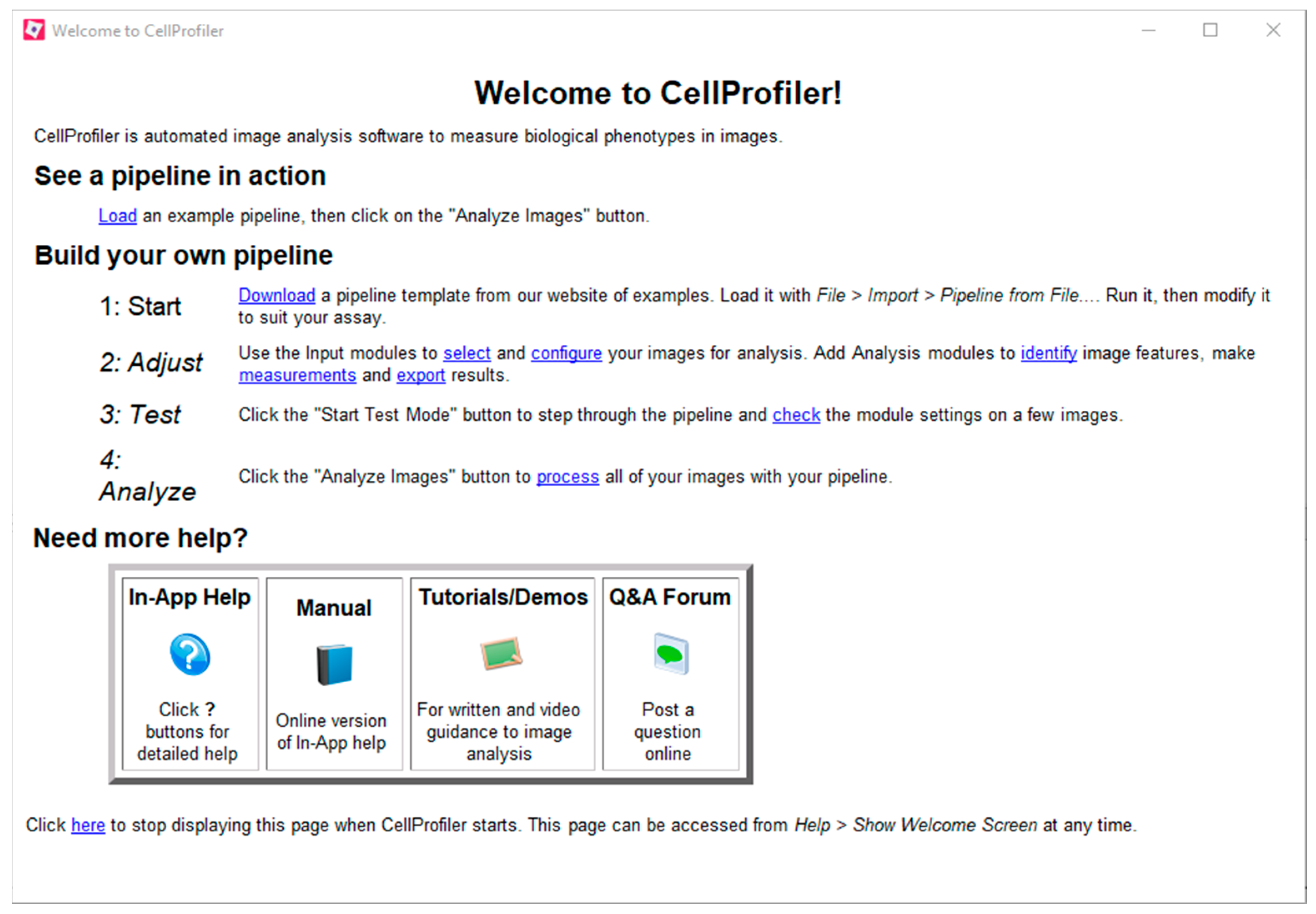
When the program opens, the Welcome Screen appears; here, a new pipeline can be created (
Figure 1). To load the pipeline, select “Open” and then the name of the file
(KidneyFibrosisComplete v2.0.cpproj, File S1). At the bottom of the program window, there are buttons to add (+), remove (−), or rearrange (
^, ˇ) a module of the pipeline. Additionally, the mode “Test” allows for the user to start the test mode by stepping through the pipeline modules one at a time by user input to check if the module settings are right, testing one or few images. The “Analyze images” mode processes all the loaded images automatically when everything is right.
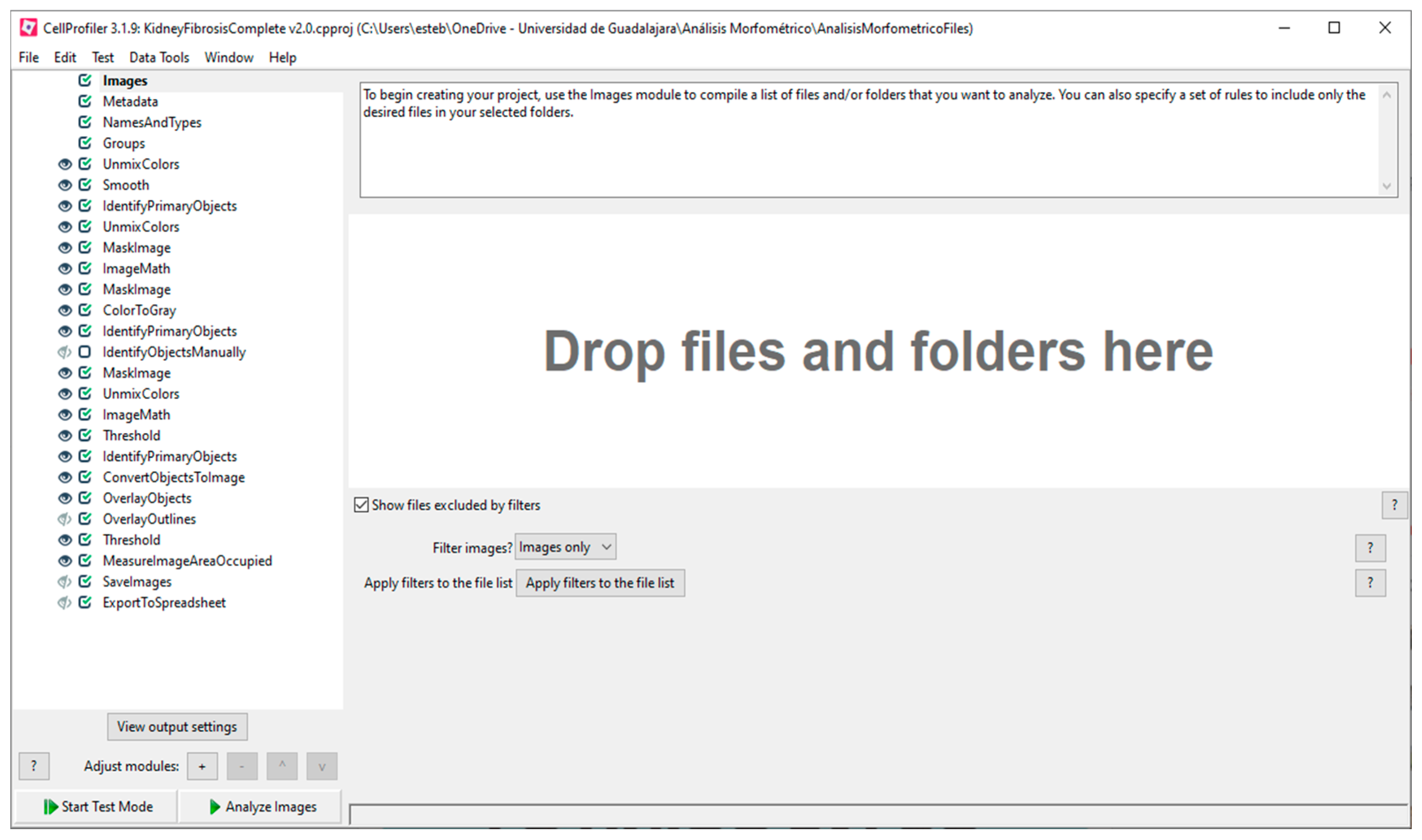
The loaded pipeline for the analysis of kidney fibrosis shows all the required modules, including the first four modules by default:
Images,
Metadata,
NamesAndTypes, and
Groups (
Figure 2). With the
Images module, a list of images can be compiled to be analyzed, including options to apply filters. The images are loaded via dragging and dropping them in the area labeled “Drop files and folders here”. If the loaded images have metadata, that information can be extracted and included in the experiment with the
Metadata module. The
NamesAndTypes module allows assigning a name to the loaded images to be used by the program such as the image type (color, grayscale, or binary mask). The
Groups module is optionally used to separate images into different groups and subsets that will be processed independently of the others based on their metadata (different image format, source, type, or screening batch date).
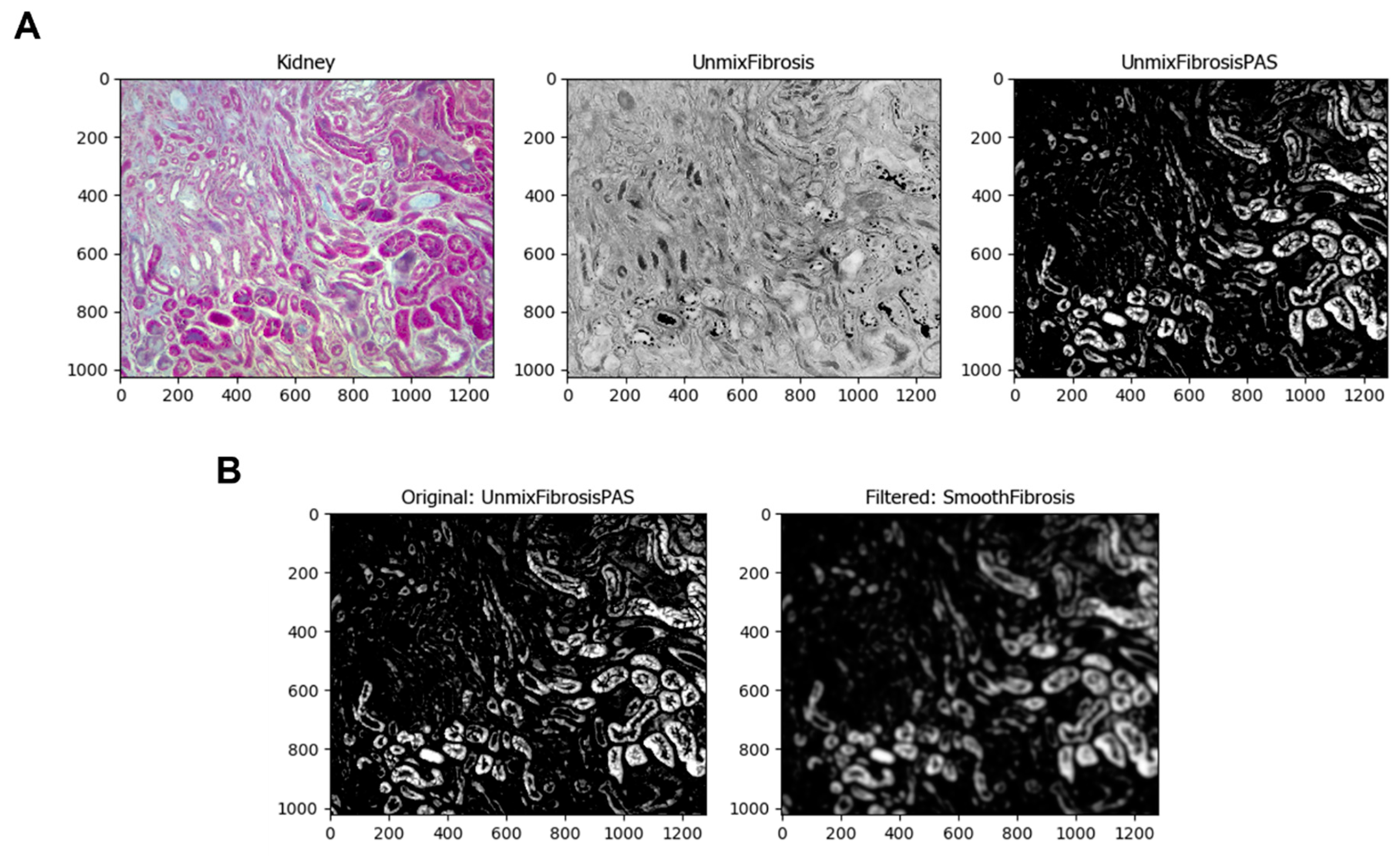
The next module is
UnmixColors, where the program can separate the colors of a specific stain using its absorbance values. This pipeline uses Hematoxylin and PAS (periodic acid Schiff) as primary and PAS as secondary (
Figure 3A). The
Smooth module smooths the images with a particular filter, in this case, the Gaussian Filter. The image processing of this module blurs the objects, delineating the lighter ones to be identified. These objects are the normal renal tubules stained by Hematoxylin, one of Masson’s dyes. The image that this module took was
UnmixFibrosisPAS, the resulting image of the
UnmixColors module (
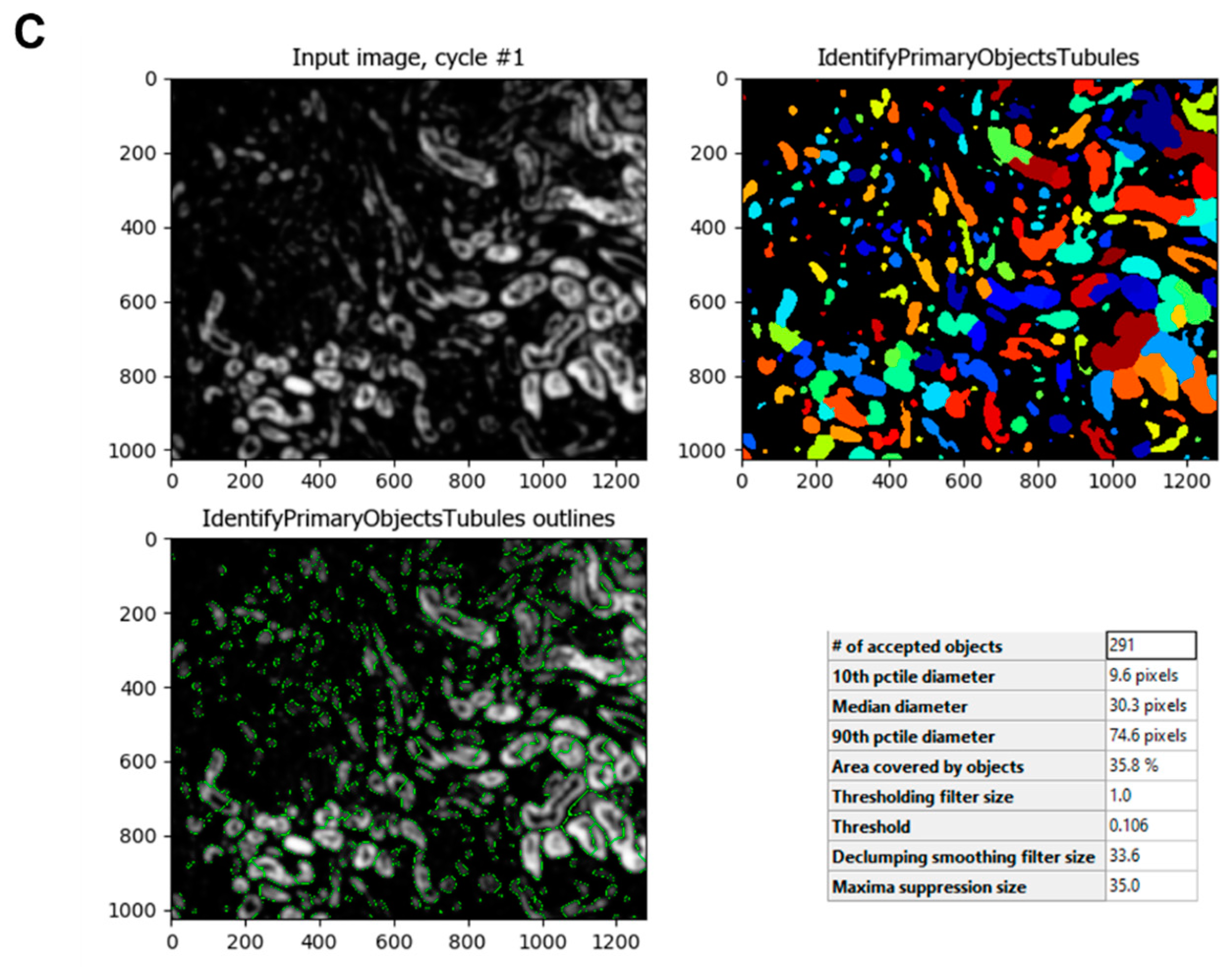
Figure 3B). To identify the normal tubules in the image, the
IdentifyPrimaryObjects module is used. Within this module, there are several settings where the typical diameter, threshold method and scale, and the method the module uses to distinguish objects can be entered. Depending on the image, these settings must be changed. The resulting process image shows the identification of the objects in green circles and the area of those in different colors. A table with various values is also displayed in the pop-up window (
Figure 3C).
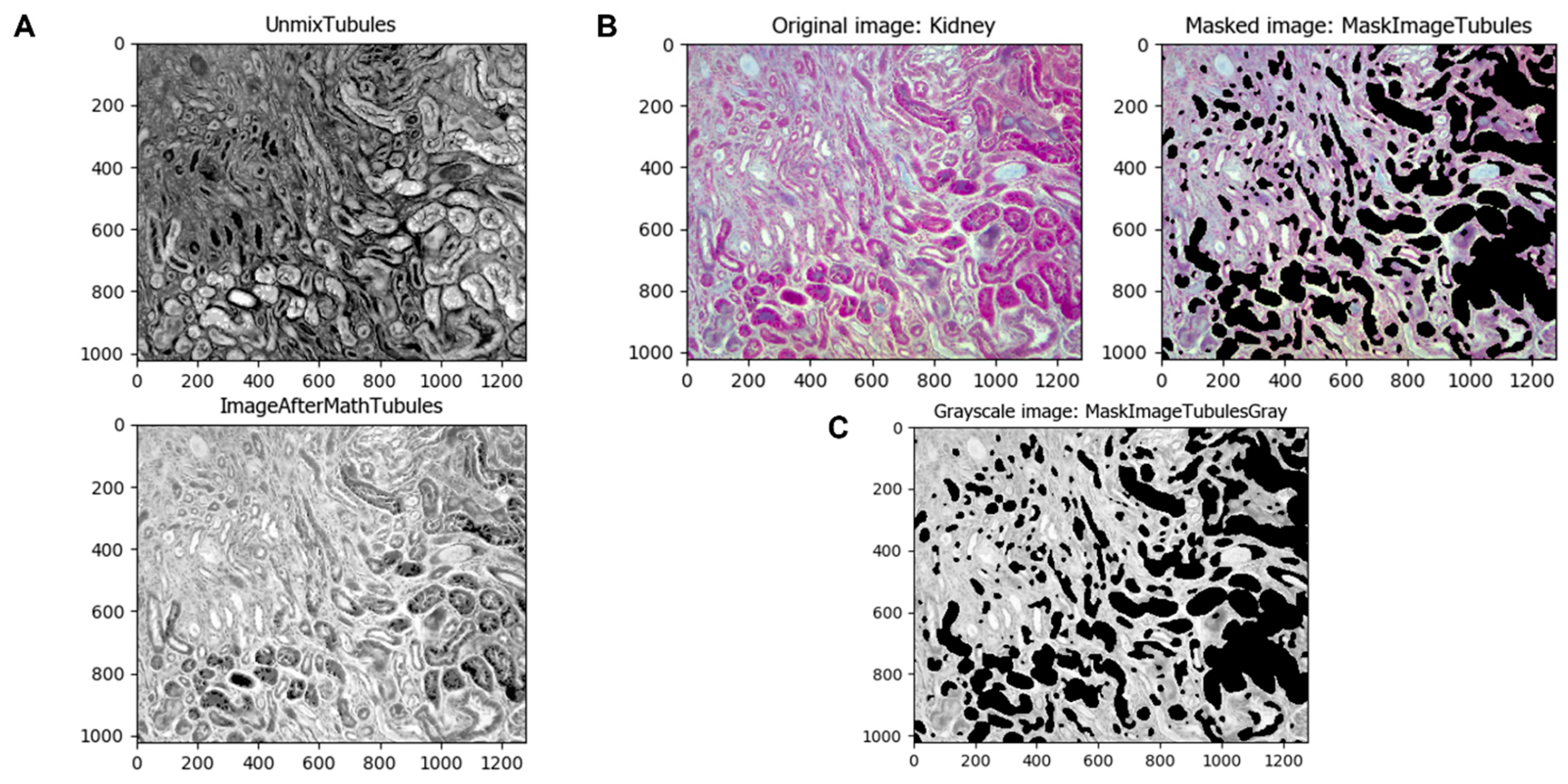
To intensify the normal kidney tubules and later separate them from the rest of the image, it is first inverted using the
ImageMath module (
Figure 4A). This module can apply other math operations to images such as add, subtract, multiply, divide, etc. The image obtained is masked with the original one using the
MaskImage module to obtain a tubule-less image and convert it to grayscale with the
ColorToGray module (
Figure 4B,C).
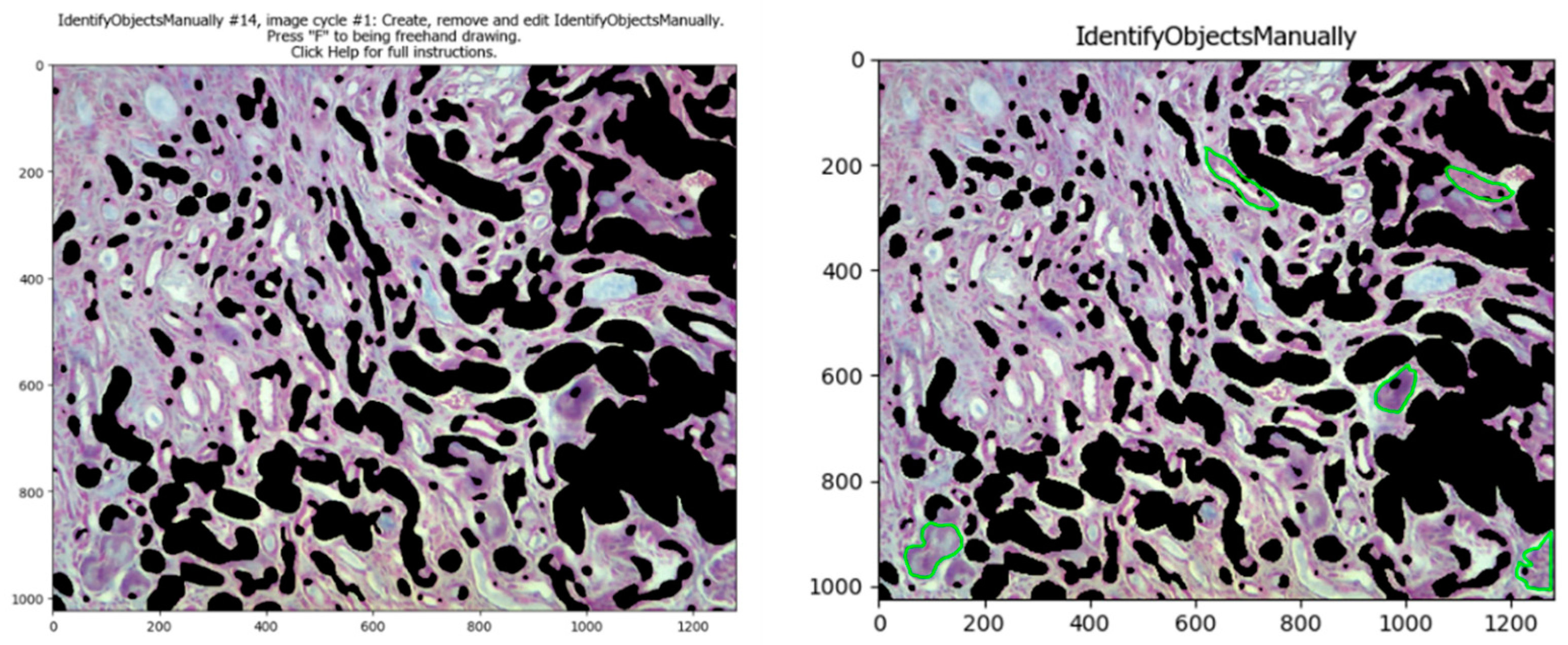
Some objects such as high stained areas or some glomeruli are difficult to select automatically and do not need to be taken into consideration for an analysis of tubulointerstitial fibrosis. If this is the case, the pipeline has the
IdentifyObjectsManually module; when it is enabled (clicking the check mark), the program lets the user select them by freehand drawing those areas. This module requires manual input, but only when it is strictly necessary; in those cases when this module is necessary to enable, is recommended to only analyze that image, and later analyze the others automatically with this module disabled (clicking the check mark again). Later, that image can be masked with the previous image with the
MaskImage module (
Figure 5).
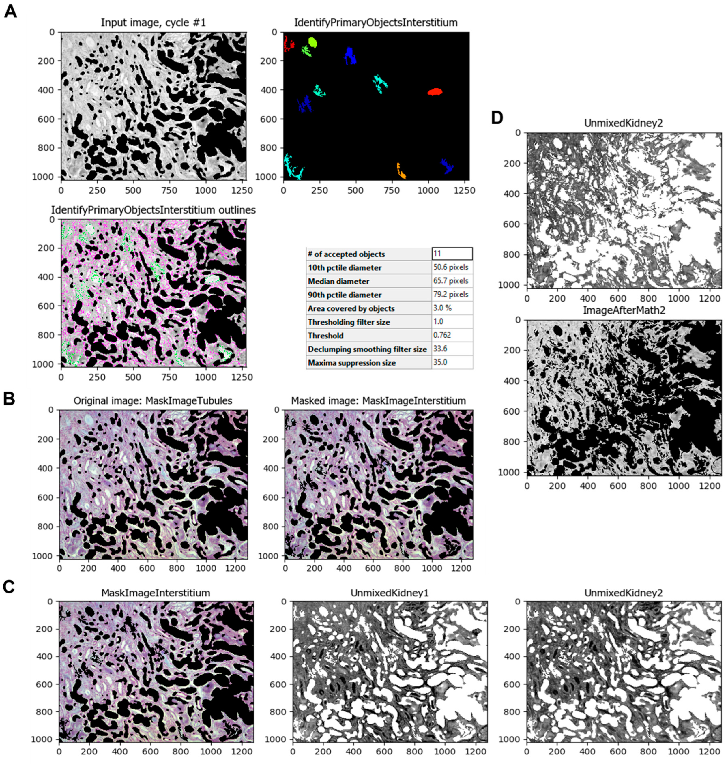
The same process is applied to the renal interstitium since the experimental model in this study produces tubulointerstitial fibrosis. Using the
IdentifyPrimaryObjects module, the program can select those areas of the normal renal interstitium and additional non-fibrotic areas as the intratubular space for better results (
Figure 6A). Once the program identifies those objects, the module
MaskImage (
Figure 6B) is applied as in the identification of the renal tubules. The module
UnmixColors is then used to separate the stains used in the samples, such as Methyl Blue (for collagen) and Ponceau-fuchsin (Masson’s Trichrome red counterstain) (
Figure 6C). Using the
ImageMath module, the resulting image is inverted (
Figure 6D).
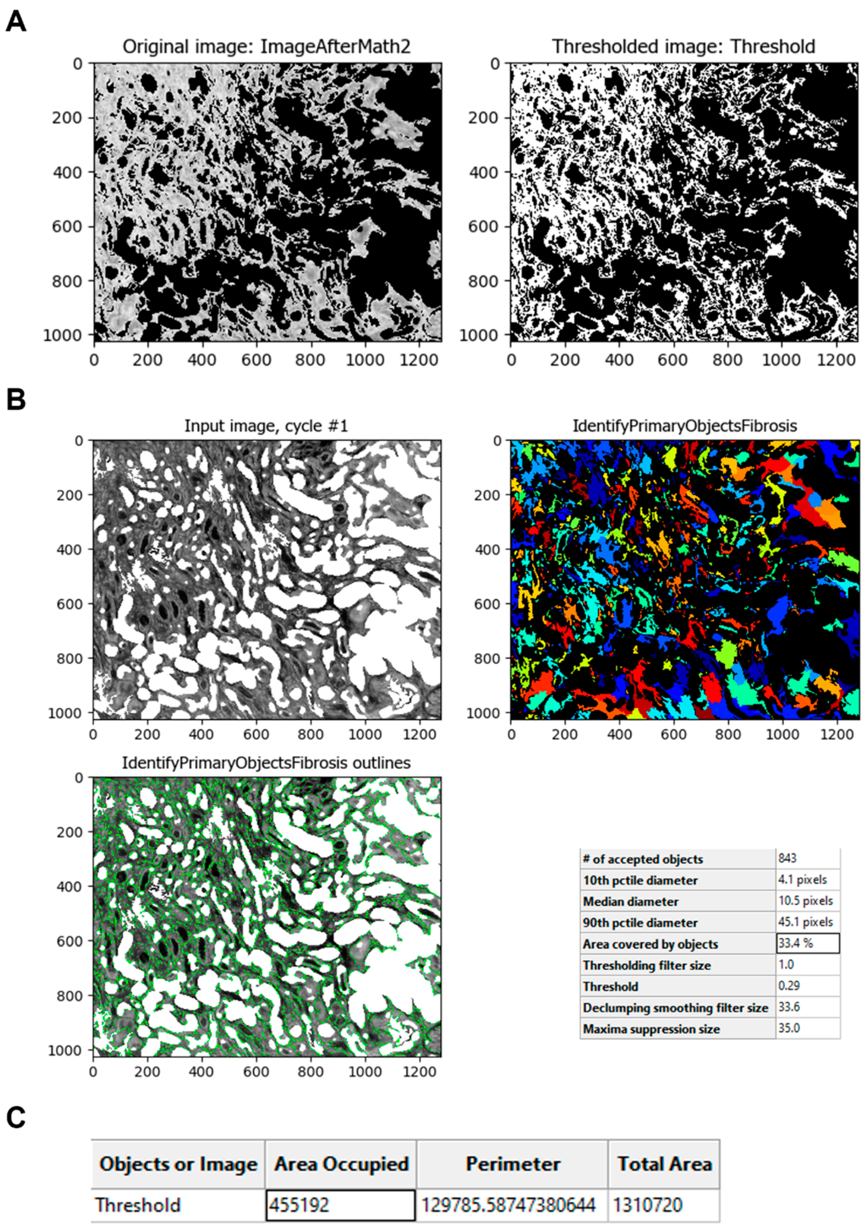
The
Threshold module is then used to obtain an image that can be processed to identify the fibrotic areas (
Figure 7A). This module calculates the threshold value of the unmasked pixels of the image. The value obtained is used to classify pixels above and below; the pixels above are treated as foreground, and the pixels below are treated as background. This value can be calculated automatically or can be adjusted by a correction factor to apply another method or strategy option to adapt more precisely across all images. The resulting process creates a binary image that shows the fibrotic area in white (1) and the background in black (0). With the resulting image, the fibrotic areas can be identified using the
IdentifyPrimaryObjects module (
Figure 7B). Once the image is thresholded, the program can measure the fibrotic area using the
MeasureImageAreaOccupied module (
Figure 7C).
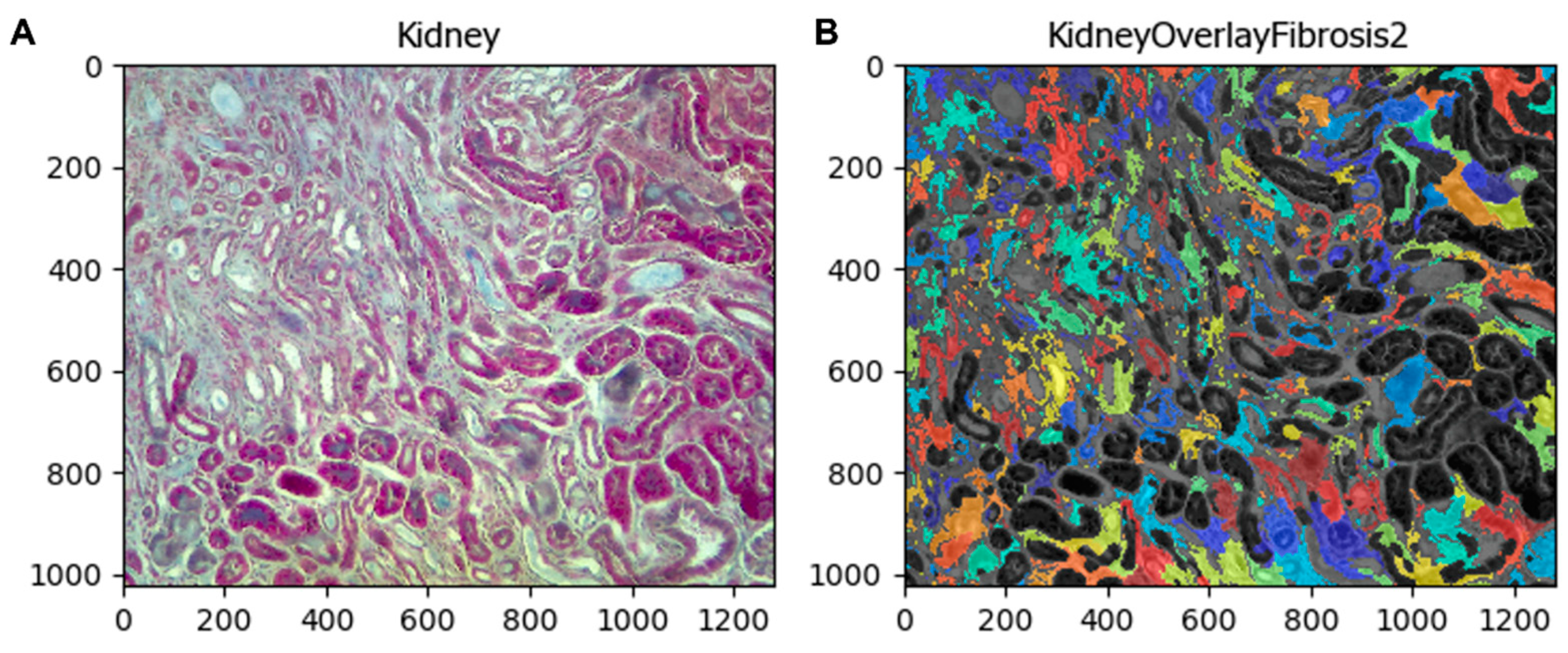
If the user wants to compare the fibrotic area identified by the pipeline with the original image, the module
OverlayObjects merges both images, maintaining the objects colored (fibrotic area) for easy comparison between them (
Figure 8).
The fibrotic area image and the data obtained can be exported as images and spreadsheets with the SaveImages and ExportToSpreadsheet modules, respectively. Once the exporting is ready, the percentage of fibrosis can be calculated using the formula: %fibrosis = (area occupied fibrosis/total area) * 100. The spreadsheet obtained has many columns filled with data; the only columns needed for calculation are “AreaOccupied_AreaOccupied_ThresholdFibrosis” (first column) and “AreaOccupied_TotalArea_ThresholdFibrosis” (third column). The percentage of fibrosis in the processed image was 34.73%.
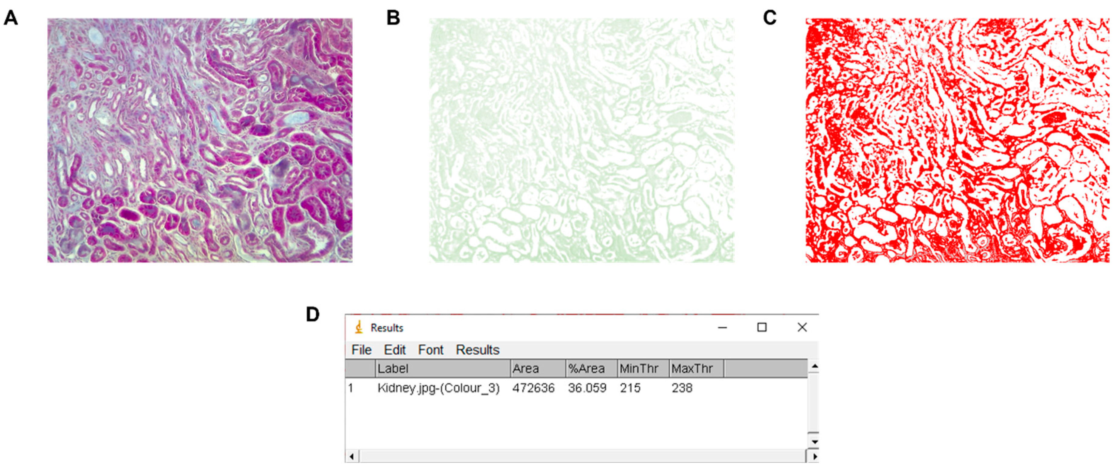
Comparison with ImageJ
To compare the results obtained with our pipeline, we also performed the analysis with the most widely used image processing software, ImageJ v.1.53 (National Institutes of Health, Bethesda, MA, USA), which employed the “Colour deconvolution” plugin [
10]. With the ImageJ program, the fibrosis index measured (fibrotic area) was 36.06% (
Figure 9).
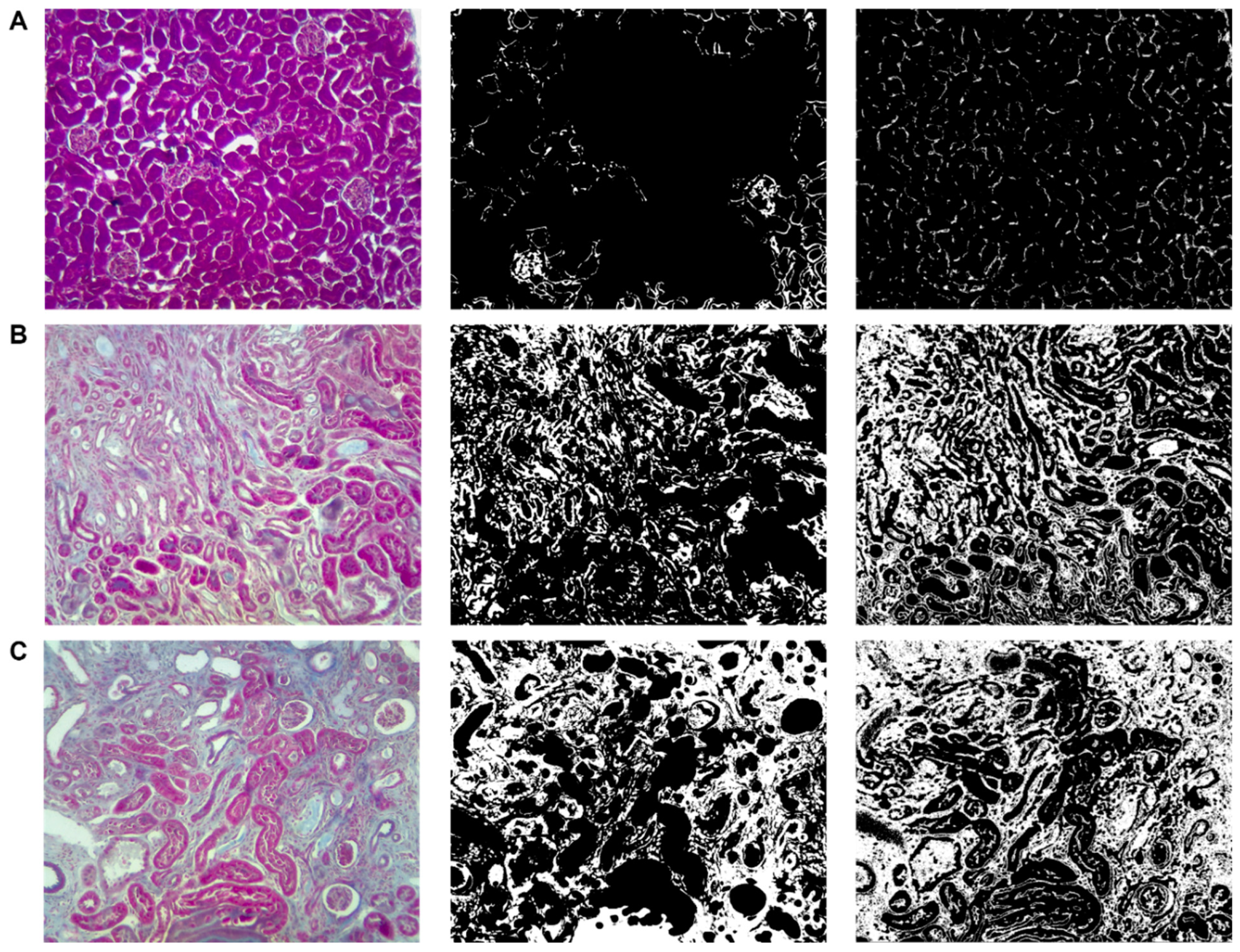
The image used to calculate the fibrosis percentage was obtained from a sample of a kidney treated with 100 mg/kg of adenine. The fibrosis area was also evaluated using samples treated with 50 mg/kg of adenine and the vehicle as control (
Figure 10).
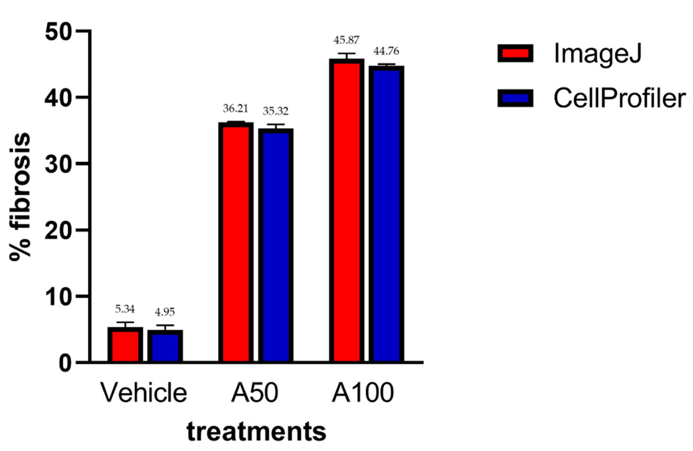
No significant statistical differences were found between the fibrosis percentage in the measured samples using both CellProfiler™ and ImageJ programs (
Figure 11).
4. Discussion
In recent years, CKD has risen as one of the most prominent health problems in the world [
1]. The last stage of kidney damage by CKD is fibrosis, an exacerbated extracellular matrix deposition that decreases kidney function [
2]. In this sense, an increased number of in vivo studies are being performed in the field of nephrology; most of them report the assessment of the percentage of fibrosis in the kidney tissue using hundreds of images on experimental animal models [
4,
8,
9,
11,
12,
13,
14] or renal biopsies [
15]. However, the measurement of fibrosis in that scenario is laborious when it is done using a manual approach, such as a score determined by a pathologist or employing a non-automated computer program [
4,
11,
16].
Recently, a computerized approach to image analysis has been gaining prominence, new methods are being developed, and some are more sophisticated than others. Although there are better approaches such as artificial intelligence [
17] and machine learning [
18] that use convolutional neural networks trained to learn how to interpret the results of a given sample, reproducing the pathologist visual assessment [
19,
20,
21,
22], there are also more straightforward approaches such as image processing software. One of the most used is the free software ImageJ [
13,
23,
24,
25,
26,
27] and, more effectively, automated software such as CellProfiler™.
The pipeline presented in this article helps analyze kidney fibrosis in Masson’s Trichrome stained images and quickly obtain the fibrotic area without needing complicated scripting or knowledge of specialized software. Our approach gives similar results to the ones obtained with ImageJ, but automatically, with the option of batch processing hundreds of images. The percentage of the fibrotic area is more accurate than the one obtained with ImageJ because the pipeline can identify renal structures as tubules, glomeruli, or vessels with high stained areas. Therefore, it is normal to expect a higher fibrosis percentage using ImageJ than the pipeline; otherwise, ImageJ requires more time fine-tuning every image to eliminate high stained areas with a background correction step for subtracting them. Another benefit of this pipeline is the plethora of options in every module to adapt more precisely to different staining qualities and intensities, some of which ImageJ does not have. Even though ImageJ has the macro ability, it applies the same values, especially in the threshold calculation, to all samples since the macros are pre-built procedures that run as defined steps that do not adapt to every image.
On the contrary, CellProfiler™ modules adapt automatically to variations in images. Furthermore, the threshold values are calculated depending on the intensity or other characteristics of the image. All of this helps to improve scientific reproducibility [
6].
Regarding time, using ImageJ, the analysis can take around 5–10 min per image sample; the most time-consuming step is determining the threshold value. On the other hand, CellProfiler™ can analyze around 20–30 image samples in the same time, depending on the computer’s hardware specifications. Although the resolution does not greatly affect the results of the pipeline, the time required to analyze a high-resolution image increases dramatically. In this regard, resolution ranging from 1024 × 768 (1.3 megapixels) to 2048 × 1536 (3.1 megapixels) is ideal to analyze images with this pipeline to obtain fast results. In terms of the validation of the pipeline described here, it was applied to another work by our group [
28] where we used 800 images of stained slides to evaluate the percentage of tubulointerstitial fibrosis on an animal model of CKD.
Even though this pipeline measures the fibrotic tissue area in stained slides only in those areas of tubulointerstitial fibrosis, it does not distinguish normal fibrotic tissue (connective tissue of basement membranes) from pathological fibrotic tissue. In this sense, workarounds can be made to overcome this limitation and challenge, such as subtracting the fibrotic area calculated previously from a control sample or combining Masson’s Trichrome with PAS staining. This method is made by deriving a differential staining area by subtraction morphometry [
15,
29] and using this pipeline on that derived image. Alternatively, polarized Sirius Red staining (specific for collagen types I and III) can be used.
It is important to note that the settings values of every module presented here must be changed to adapt to different image lots, depending on the intensity of the colors of the Masson’s Trichrome staining. Grouping images from the same animal or collection date is unnecessary because the pipeline modules adapt to different images obtained from different animals. On the contrary, other criteria such as animal condition, reagent lot, and staining process date can be important for grouping when the user needs to change the settings in some modules to better adapt to differences in staining. However, once one representative image is analyzed and the area of fibrosis correctly determined, the pipeline does all the processing work for the rest of the images in the lot. In this sense, it is essential to analyze the same group of images with the same image acquisition software options of the microscope or camera to avoid variability in staining intensity. The most important setting to change in the pipeline is the threshold correction factor in the IdentifyPrimaryObjects and Threshold modules.
This pipeline was created with the purpose of morphometrically analyzing samples taken from experimental animal models, especially murine models of CKD. It is limited to quantifying tubulointerstitial fibrosis and not glomerulonephritis or glomerulosclerosis in animal models because glomeruli are excluded for analysis. However, in the future, it is intended to obtain patient samples to validate and subsequently use them in human-derived samples. Additionally, we intend to expand its use and apply machine learning methods inside the pipeline to obtain better results quantifying kidney fibrosis.


 ,
, 


