Impact of Second-Order Slip and Double Stratification Coatings on 3D MHD Williamson Nanofluid Flow with Cattaneo–Christov Heat Flux

Abstract

The present research examines the impact of second-order slip with thermal and solutal stratification coatings on three-dimensional (3D) Williamson nanofluid flow past a bidirectional stretched surface and envisages it analytically. The novelty of the analysis is strengthened by Cattaneo–Christov (CC) heat flux accompanying varying thermal conductivity. The appropriate set of transformations is implemented to get a differential equation system with high nonlinearity. The structure is addressed via the homotopy analysis technique. The authenticity of the presented model is verified by creating a comparison with the limited published results and finding harmony between the two. The impacts of miscellaneous arising parameters are deliberated through graphical structures. Some useful tabulated values of arising parameters versus physical quantities are also discussed here. It is observed that velocity components exhibit an opposite trend with respect to the stretching ratio parameter. Moreover, the Brownian motion parameter shows the opposite behavior versus temperature and concentration distributions.

1. Introduction

The heat transfer phenomenon plays a vital role when the temperature varies between different bodies or parts of the same body. Heat can be transferred by three methods: convection of fluids, conduction in solids, and radiation. To examine body heat transfer, the principle of heat transfer can be applied to the human body. Here, we can quote one example: the metal pan is used to transfer heat from the stove to food. Some applications of heat transfer are cooking food over metal pots, boiling milk in metal pots, and thermal treatment of pain by a hot water bag. Straughan [1] considered the Cattaneo–Christov (CC) model for heat flux and thermal convection over a Newtonian fluid. Khan et al. [2] analyzed it numerically by engaging the bvp4c MATLAB-based function on a Sisko fluid flow accompanied by generalized Fick’s and Fourier’s laws over a nonlinear stretched surface. Hayat et al. [3] examined analytically the magnetohydrodynamics (MHD) flow of Jeffrey fluid past a variable thick surface via the impacts of the chemical reaction and the CC model in a stratified medium. Waqas et al. [4] investigated the CC heat flux model for energy equation formulation rather than Fourier’s law of heat conduction. It was observed that a variable thermal conductivity remains inversely proportional to a temperature profile. The Soret–Dufour effects on walls with the second-grade fluid flow between inclined parallel plain walls were inspected by Khan et al. [5]. Heat transfer characteristics of the incompressible flow of the second-grade fluid flow produced by a stretching sheet were analyzed by Ghadikolaei et al. [6]. Khan et al. [7] investigated the behavior of homogenous–heterogeneous reactions against heat transfer flow due to a stretching sheet. They noticed that homogenous–heterogeneous reactions reduce fluid concentration.

In modern engineering processes, especially in metallurgical engineering and metalworking practices, the role of MHD is fundamental for electrically conducting fluids. The magnetic field function is crucial in cooling the hot plasma inside a nuclear reactor vessel. Similarly, the magnetic field is employed for the mixing of metals inside an electrical furnace [8]. Chamkha et. al. [9] analyzed the magnetic field effect on the mixed convection unsteady flow in an ambient fluid past a cone rotating with an unsteady angular velocity. Pullepu et al. [10] analyzed the free convection flow with variable surface temperature over a nonisothermal vertical cone. Akbar et al. [11] examined the two dimensional (2D) electrically conducting flow of the hyperbolic tangent fluid past a stretching surface. They observed that an increment in the Hartmann number decelerates the fluid velocity in the domain of the stretching sheet. Seini et al. [12] highlighted the magnetic field impact over a stretching surface accompanied by the appearance of slip velocity near the stagnation point flow. They perceived that the impact of the magnetic field is more significant on the velocity profile. Ravindran et al. [13] considered the impact of a transverse magnetic field and heat generation and absorption on time-dependent mixed convection flow over a porous cone with a chemical reaction. Boland et al. [14] simulated MHD flow of viscous fluid over a circular cylinder covered with a permeable layer. They adopted the Darcy–Brinkman–Forchheimer model to study the flow inside a porous medium. Ellahi et al. [15] investigated the influence of a Hall current on MHD Jeffrey fluid flow over a nonuniform duct. Mishra et al. [16] explored heat transfer and mass in the appearance of a magnetic field of viscoelastic fluid flow. They determined that the behavior of the magnetic field against the velocity profile is opposite to temperature distribution and concentration profiles. Hussain et al. [17] analyzed numerically the influence of the applied magnetic field on a non-Newtonian fluid flow past a stretching surface.

Nanofluids are vital in many engineering applications, such as in biomedical engineering and many chemical processes. Nanofluid is composed of nanometer-sized particles with a diameter of less than 100 nm and some conventional fluid. The basic aim of using nanofluids is to upgrade the heat transfer and thermal conductivity to attain better cooling. Khan et al. [18] highlighted nanofluid flow over a stretching sheet. Makinde [19] extended the work of Khan et al. [18] to convective boundary condition in nanofluid flow. Nadeem et al. [20] analyzed the second-grade nanofluid (nonorthogonal stagnation point) flow in the direction of the stretching surface. The impact of the variable magnetic field on the nanofluid flow between two disks was explored by Hayami et al. [21]. They found the analytical solution via the homotopy perturbation method and observed that the temperature of the boundary layer thickness decreases with the increase of the Brownian motion parameter and thermophoretic factor. Nanofluid flow in a permeable medium over a convectively heated permeable shrinking sheet was examined by Hayat et al. [22]. Sheikholeslami et al. [23,24] considered the behavior of the magnetic field on the free and forced convection flow of nanofluids respectively by making use of the two-phase model. Hassan et al. [25] elaborated on convective transport of heat transfer in a nanofluid through a porous medium. They concluded that convective heat transfer is improved by nanoparticle concentration, and the magnetic field impacts second-order slip flow. Nayak et al. [26] focused on the numerical solution of the three-dimensional (3D) nanofluid flow with nonlinear thermal radiation with convective conditions and slip. Hosseini et al. [27] observed the nanofluid MHD flow in a microchannel heat sink via the KKL (Koo–Kleinsteuer–Li) model. They noticed that the interaction between nanoparticles and the solid phase enhances the Nusselt number. In recent years, several scientists have used nanofluid heat transfer in their studies [28,29,30,31,32,33,34].

Fluids are basically divided into two groups: Newtonian [35] and non-Newtonian fluids [36]. Fluids that abide by Newton’s law of viscosity are termed Newtonian fluids. However, a contradiction to Newton’s law of viscosity is observed in non-Newtonian fluids. Applications of non-Newtonian fluids may be found in many industrial and engineering areas, glass fiber, hot rolling, casting, and paper production. Amongst many non-Newtonian fluids, Williamson fluid possesses shear thinning property (i.e., viscosity tends to decrease when shear stress increases). Abundant articles may be found in the literature that highlight the importance of Williamson fluid in numerous scenarios. Ramzan et al. [37] examined Williamson nanofluid flow over a Riga plate. They found that with an increase in Williamson fluid parameter velocity, distribution decreases. Ramzan et al. [38] also analyzed the numerical solution of the 2D MHD stagnation point of Williamson fluid flow under the effect of homogeneous–heterogeneous reactions over a linearly stretched surface and found opposite behavior of temperature and velocity distribution against the Williamson fluid parameter. Nadeem et al. [39,40] analyzed the 2D Williamson fluid flow over a stretching sheet considering the influence of nanosized particles, also characterized as Williamson nanofluid. They studied the Williamson nanofluid peristaltic flow in a curved channel, including compliant walls.

Homotopy analysis method (HAM) was suggested by Liao [41] in 1992 to solve highly nonlinear differential equations. This technique has an edge over the rest of the contemporary techniques. HAM is one of the best and simplest technique for obtaining the convergent series solution for weakly, as well as, highly nonlinear differential equations. This technique includes the concept of homotopy from topology. HAM is used for finding a convergent series solution with high nonlinearity. Homotopy discriminates itself from other methods in the following ways:

• Freedom to choose large or small parameters;
• Guaranteed series solution convergence; and
• Freedom to choose linear operators and base function.

There have been many attempts in the literature to discuss the varied fluid problems utilizing the homotopy analysis method [42,43,44,45,46,47,48,49].

A literature review discloses that copious literature may be quoted in the case of 2D non-Newtonian flows. Less work is available on 3D geometries, and this group becomes narrower if we talk about 3D Williamson nanofluid flows. The subject matter of 3D MHD flow of Williamson nanofluid over a bidirectional stretched surface with second-order slip and double stratification is even more rarely discussed. The structure of this paper is as follows: In Section 2, we present the mathematical model. In Section 3, Section 4 and Section 5, we discuss the homotopic scheme in detail with zeroth and mth order solutions. In Section 6, we address the convergence analysis. In Section 7, we present the results and discuss their physical importance, and finally, we provide concluding remarks.

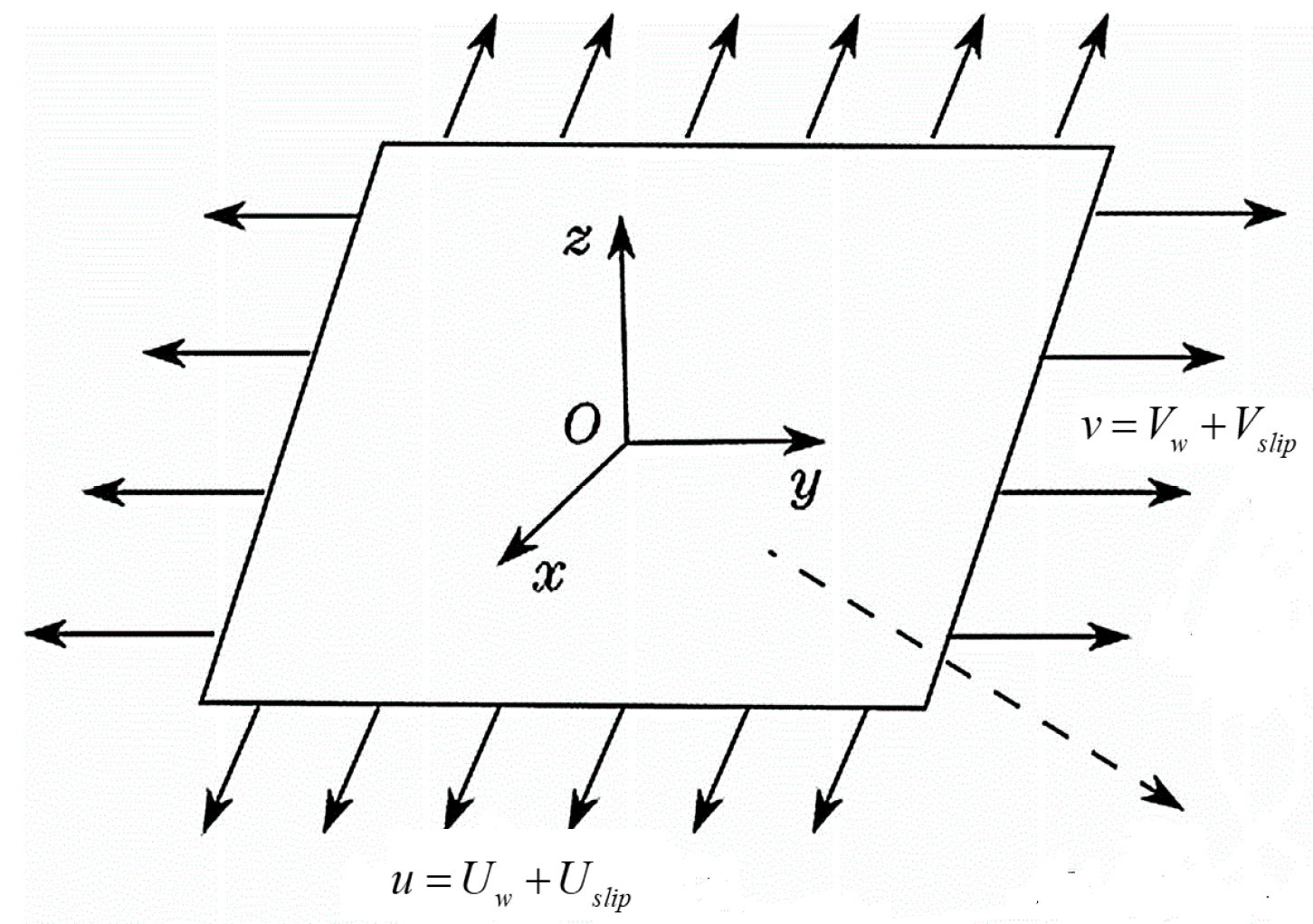
2. Mathematical Modeling

Here, we consider the steady 3D Williamson nano liquid flow with velocities of $U_w=ax$ in the x-direction and $V_w=by$ in the y-direction, respectively, over a bidirectional extended sheet. While a and b are constants (Figure 1), concentration buoyancy force and thermal are used by the fluid with double stratification phenomena to study heat and mass transfers.

The following are the governing boundary layer equations:

$$u_x+v_y+w_z=0$$

(1)

$$u{u}_x+v{u}_y+w{u}_z=\nu u_{zz}+\sqrt{2}\Gamma \nu u_z{u}_{zz}-\frac{\sigma B_0^2}{\rho }u+\left[\begin{array}{l}g[{\alpha }_1(T-T_{\infty })+{\alpha }_2{(T-T_{\infty })}^2]+\\ g[{\alpha }_3(\mathrm{C}-C_{\infty })+{\alpha }_4{(\mathrm{C}-C_{\infty })}^2]\end{array}\right]$$

(2)

$$u{v}_x+v{v}_y+w{v}_z=\nu v_{zz}+\sqrt{2}\Gamma \nu v_z{v}_{zz}-\frac{\sigma B_0^2}{\rho }v$$

(3)

$$q+{\lambda }_E(q_t+V.\nabla q-q.\nabla V+(\nabla .\mathrm{V})\mathrm{q})=-\nabla (\mathrm{k}\mathrm{T})$$

(4)

$$J+{\lambda }_C({\mathrm{J}}_t+V.\nabla J-J.\nabla V+(\nabla .\mathrm{V})\mathrm{J})=-D_B\nabla \mathrm{C}$$

(5)

$$q+{\lambda }_E(V.\nabla q-q.\nabla V)=-\nabla (kT)$$

(6)

$$J+{\lambda }_C(V.\nabla J-J.\nabla V)=-D_B\nabla C$$

(7)

under the supervision of above-mentioned consideration and the impression of thermophoresis and Brownian-motion, Equations (6) and (7) takes the form:

$$u{T}_x+v{T}_y+w{T}_z+{\lambda }_E{\varphi }_E=\frac{1}{\rho c_p}\frac{\partial }{\partial z}(k{T}_z)+\tau [D_B{C}_z{T}_z+\frac{D_T}{T_{\infty }}{(T_z)}^2$$

(8)

$$u{C}_x+v{C}_y+w{C}_z+{\lambda }_C{\varphi }_C=D_B{C}_{zz}+\frac{D_T}{T_{\infty }}{T}_{zz}$$

(9)

where

$${\varphi }_E=u^2{T}_{xx}+v^2{T}_{yy}+w{T}_{zz}+2uv{T}_{xy}+2uw{T}_{xz}+2vw{T}_{yz}+\left[\begin{array}{l}(u{u}_x+v{u}_y+w{u}_z)T_x+\\ (u{v}_x+v{v}_y+w{v}_z)T_y+\\ (u{w}_x+v{w}_y+w{w}_z)T_z\end{array}\right]$$

(10)

$${\varphi }_C=u^2{C}_{xx}+v^2{C}_{yy}+w{C}_{zz}+2uv{C}_{xy}+2uw{C}_{xz}+2vw{C}_{yz}+\left[\begin{array}{l}(u{u}_x+v{u}_y+w{u}_z){\mathrm{C}}_x+\\ (u{v}_x+v{v}_y+w{v}_z){\mathrm{C}}_y+\\ (u{w}_x+v{w}_y+w{w}_z){\mathrm{C}}_z\end{array}\right]$$

(11)

following boundary conditions supports the above-mentioned system of equations:

$$\begin{array}{l}u=U_w+U_{slip}v=V_w+V_{slip}w=0\\ T=T_w=T_0+d_{1}xC=C_w=C_0+d_{2}x\mathrm{at}z=0\\ u\to 0v\to 0T\to T_{\infty }=T_0+e_{1}xC\to C_{\infty }=C_0+e_{2}x\mathrm{as}z\to \infty \end{array}$$

(12)

here

$$U_{slip}=\frac{2}{3}\left(\frac{3-\alpha l^3}{\alpha }-\frac{3}{2}\frac{1-l^2}{K_n}\right)\Lambda u_z-\frac{1}{4}\left(l^4+\frac{2}{K_n^2}(1-l^2)\right){\Lambda }^2{u}_{zz}=A{u}_z+B{u}_{zz}$$

(13)

$$V_{slip}=\frac{2}{3}\left(\frac{3-\alpha l^3}{\alpha }-\frac{3}{2}\frac{1-l^2}{K_n}\right)\Lambda v_z-\frac{1}{4}\left(l^4+\frac{2}{K_n^2}(1-l^2)\right){\Lambda }^2{v}_{zz}=C{v}_z+D{v}_{zz},$$

(14)

where $A=\frac{2}{3}\left(\frac{3-\alpha l^3}{\alpha }-\frac{3}{2}\frac{1-l^2}{K_n}\right)\Lambda$, $B=-\frac{1}{4}\left(l^4+\frac{2}{K_n^2}(1-l^2)\right){\Lambda }^2$, $C=\frac{2}{3}\left(\frac{3-\alpha l^3}{\alpha }-\frac{3}{2}\frac{1-l^2}{K_n}\right)\Lambda$, $D=-\frac{1}{4}\left(l^4+\frac{2}{K_n^2}(1-l^2)\right){\Lambda }^2$, $l=\min \left[\frac{1}{K_n},1\right]$, α describes momentum accommodation coefficient and varies from $0\le \alpha \le 1$ $K_n$ denotes Knudsen number and $\Lambda$ denotes molecular mean free path. On the basis of definition of $l$, we found for any particular estimates of $K_n$ we own $1\ge l\ge 0.$ The molecular mean free path is always positive. Therefore, we know that B, D ˂ 0 and C and A are positive.

To solve Equations (1),(3) and (8),(9), following similarity transformations are introduced:

$$\begin{array}{l}u=axf\prime (\eta )v=ayg\prime (\eta )w=-\sqrt{a\nu }\left(f(\eta )+g(\eta )\right)\\ \theta (\eta )=\frac{T-T_{\infty }}{T_w-T_{\infty }}\varphi (\eta )=\frac{C-C_{\infty }}{C_w-C_{\infty }}\eta =\sqrt{\frac{a}{\nu }}z\end{array}$$

(15)

here, $f$, $g$, $\theta$ and $\varphi$ are the non-dimensional form for both velocities, temperature and the concentration.

Condition for incompressibility is self-satisfied and Equations (2),(3) and (8),(9) reduce to:

$$f‴-f{\prime }^2+(f+g)f″+Wef″f‴+\lambda (1+{\beta }_2\theta )\theta +\lambda Nr(1+{\beta }_3\varphi )\varphi -Haf\prime =0$$

(16)

$$\mathrm{g}‴-g{\prime }^2+(f+g)\mathrm{g}″+Weg″\mathrm{g}‴-Ha\mathrm{g}\prime =0$$

(17)

$$\begin{array}{l}(1+\epsilon \theta )\theta ″+\epsilon {\theta }^{\prime 2}+\mathrm{Pr}{N}_b\theta \prime \varphi \prime +\mathrm{Pr}{N}_t{\theta }^{\prime 2}-\mathrm{Pr}f\prime (S_1+\theta )+\\ \mathrm{Pr}(f+g)\theta \prime -{\delta }_t\mathrm{Pr}\left(\begin{array}{l}{(f+g)}^2\theta ″-2f\prime \theta \prime (f+g)+\left(f{\prime }^2-f″(f+g)\right)(S_1+\theta )\\ +(f+g)(f\prime +g\prime )\theta \prime \end{array}\right)=0\end{array}$$

(18)

$$\begin{array}{l}\varphi ″+\frac{N_t}{N_b}\theta ″-\mathrm{Pr}Lef\prime ({\mathrm{S}}_2+\varphi )+\mathrm{Pr}Le(f+g)\varphi \prime -\\ \mathrm{Pr}Le{\delta }_c\left(\begin{array}{l}{(f+g)}^2\varphi ″-2f\prime (f+g)\varphi \prime +\left(f{\prime }^2-f″(f+g)\right)(S_2+\varphi )+\\ (f+g)(f\prime +g\prime )\varphi \prime \end{array}\right)\end{array}$$

(19)

and boundary conditions hold the form

$$\begin{array}{l}f(0)=0f\prime (0)=1+{\gamma }_{1}f″(0)+{\gamma }_{2}f‴(0)\mathrm{g}(0)=0\\ \mathrm{g}\prime (0)=1+{\gamma }_3\mathrm{g}″(0)+{\gamma }_4\mathrm{g}‴(0)\theta (0)=1-{\mathrm{S}}_1\varphi (0)=1-{\mathrm{S}}_2\\ \mathrm{f}\prime (\infty )\to 0\mathrm{g}\prime (\infty )\to 0\theta (\infty )=0\varphi (\infty )=0asz\to \infty \end{array}$$

(20)

where the parameters given above are defined as follows:

$$\begin{array}{l}\lambda =\frac{G{r}_x}{{\mathrm{Re}}_x^2}G{r}_x=\frac{g{\beta }_T(T_w-T_{\infty })x^3}{{\nu }^2}{\mathrm{Re}}_x=\frac{u_{w}x}{\nu }Nr=\frac{{\alpha }_3(C_w-C_0)}{{\alpha }_1({\mathrm{T}}_w-T_0)}{\mathrm{S}}_1=\frac{e_1}{d_1}\\ {\gamma }_1=A\sqrt{\frac{a}{\nu }}{\gamma }_2=B\frac{a}{\nu }{\gamma }_3=C\sqrt{\frac{a}{\nu }}{\gamma }_4=D\frac{a}{\nu }{\beta }_2=\frac{{\alpha }_2}{{\alpha }_1}(T_w-T_0)\beta =\frac{b}{a}\\ {\beta }_3=\frac{{\alpha }_4}{{\alpha }_3}(C_w-C_0){\alpha }_1={\beta }_{T}We=U_w\Gamma \sqrt{\frac{2c}{\nu }}\mathrm{Pr}=\frac{\mu c_p}{k}Ha=\frac{\sigma B_0^2}{\rho a}{\mathrm{S}}_2=\frac{e_2}{d_2}\\ Le=\frac{\alpha }{D_B}Nt=\frac{\tau D_T(T_w-T_0)}{T_{\infty }\nu }Nb=\frac{\tau D_B({\mathrm{C}}_w-C_0)}{T_{\infty }\nu }{\delta }_c={\lambda }_{C}a{\delta }_t={\lambda }_{E}a\end{array}$$

(21)

$C_{fx}$ is the coefficients of Skin friction in x- and $C_{fy}$ in the y-direction are represented as follows:

$$C_{fx}=\frac{{\tau }_{wx}}{\rho U_w^2}{C}_{fy}=\frac{{\tau }_{wy}}{\rho U_w^2}$$

(22)

$$\mathrm{where}{{\tau }_{wx}|}_{z=0}=u_z+\frac{\Gamma }{\sqrt{2}}{({\mathrm{u}}_z)}^2\mathrm{and}{{\tau }_{wy}|}_{z=0}=v_z+\frac{\Gamma }{\sqrt{2}}{({\mathrm{v}}_z)}^2$$

(23)

Coefficients of Skin friction in dimensionless forms are:

$$\begin{array}{l}{C}_{fx}{\mathrm{Re}}^{\raisebox{1ex}{$1$}\!\left/ \!\raisebox{-1ex}{$2$}\right.}={[f″+\frac{We}{2}{(f″)}^2]}_{\eta =0}\\ C_{fy}{\mathrm{Re}}^{\raisebox{1ex}{$1$}\!\left/ \!\raisebox{-1ex}{$2$}\right.}={[\mathrm{g}″+\frac{We}{2}{(\mathrm{g}″)}^2]}_{\eta =0}\end{array}$$

(24)

3. Homotopic Solutions

For the considered problem, $(L_f,L_{g,}{L}_{\theta },L_{\varphi })$ are the linear operators and $(f_0,g_0,{\theta }_0,{\varphi }_0)$ are the initial guesses expressed in the following form:

$$\begin{array}{l}{f}_0(\eta )=\frac{A}{1+{\gamma }_1-{\gamma }_2}(1-\exp (-\eta ))g_0(\eta )=\frac{\beta }{1+{\gamma }_3-{\gamma }_4}(1-\exp (-\eta ))\\ \mathrm{where}1+{\gamma }_1-{\gamma }_2\ne 01+{\gamma }_3-{\gamma }_4\ne 0\\ {\theta }_0(\eta )=(1-S_1)(1-\exp (-\eta )){\varphi }_0(\eta )=(1-S_2)(1-\exp (-\eta ))\end{array}$$

(25)

$$\begin{array}{l}{L}_f(f)=\frac{d^{3}f}{d{\eta }^3}-\frac{df}{d\eta }{L}_g(g)=\frac{d^{3}g}{d{\eta }^3}-\frac{dg}{d\eta }\\ L_{\theta }(\theta )=\frac{d^2\theta }{d{\eta }^2}-\theta L_{\varphi }(\varphi )=\frac{d^2\varphi }{d{\eta }^2}-\varphi \end{array}$$

(26)

these operators satisfy the following condition:

$$\begin{array}{l}{L}_f[C_1+C_2\exp (\eta )+C_3\exp (-\eta )]=0\\ L_g[C_4+C_5\exp (\eta )+C_6\exp (-\eta )]=0\\ L_{\theta }[C_9\exp (\eta )+C_{10}\exp (-\eta )]=0\end{array}$$

(27)

4. Zeroth Order Deformation

The zeroth order deformation problem is defined as follows:

$$(1-p)L_f[\stackrel{\sim }{f}(\eta ;p)-f_0(\eta )]=p{\hslash }_f{N}_f[\stackrel{\sim }{f}(\eta ;p),\stackrel{\sim }{g}(\eta ;p)]$$

(28)

$$(1-p)L_g[\stackrel{\sim }{g}(\eta ;p)-g_0(\eta )]=p{\hslash }_g{N}_g[\stackrel{\sim }{f}(\eta ;p),\stackrel{\sim }{g}(\eta ;p)]$$

(29)

$$(1-p)L_{\theta }[\stackrel{\sim }{\theta }(\eta ;p)-{\theta }_0(\eta )]=p{\hslash }_{\theta }{N}_{\theta }[\stackrel{\sim }{f}(\eta ;p),\stackrel{\sim }{g}(\eta ;p),\stackrel{\sim }{\theta }(\eta ;p),\stackrel{\sim }{\varphi }(\eta ;p)]$$

(30)

$$(1-p)L_{\varphi }[\stackrel{\sim }{\varphi }(\eta ;p)-{\varphi }_0(\eta )]=p{\hslash }_{\varphi }{N}_{\varphi }[\stackrel{\sim }{f}(\eta ;p),\stackrel{\sim }{g}(\eta ;p),\stackrel{\sim }{\theta }(\eta ;p),\stackrel{\sim }{\varphi }(\eta ;p)]$$

(31)

$$\begin{array}{l}\stackrel{\sim }{f}(0;p)=0\stackrel{\sim }{f\prime }(0;p)=1+{\gamma }_1\stackrel{\sim }{f″}(0;p)+{\gamma }_2\stackrel{\sim }{f‴}(0;p)\stackrel{\sim }{f\prime }(\infty ;p)=0\\ \stackrel{\sim }{g}(0;p)=0\stackrel{\sim }{\mathrm{g}\prime }(0;p)=\beta +{\gamma }_3\stackrel{\sim }{\mathrm{g}″}(0;p)+{\gamma }_2\stackrel{\sim }{\mathrm{g}‴}(0;p)\stackrel{\sim }{\mathrm{g}\prime }(\infty ;p)=0\\ \stackrel{\sim }{\theta }(0;p)=1-S_1\stackrel{\sim }{\theta }(\infty ;p)=0\stackrel{\sim }{\varphi }(0;p)=1-S_2\stackrel{\sim }{\varphi }(\infty ;p)=0\end{array}$$

(32)

$$\begin{array}{l}{N}_f[\stackrel{\sim }{f}(\eta ;p),\stackrel{\sim }{g}(\eta ;p)]=\frac{{\partial }^3\stackrel{\sim }{f}(\eta ;p)}{\partial {\eta }^3}-{\left(\frac{\partial \stackrel{\sim }{f}(\eta ;p)}{\partial \eta }\right)}^2+(\stackrel{\sim }{f}+\stackrel{\sim }{g})\frac{{\partial }^2\stackrel{\sim }{f}(\eta ;p)}{\partial {\eta }^2}+\\ We\frac{{\partial }^2\stackrel{\sim }{f}(\eta ;p)}{\partial {\eta }^2}\frac{{\partial }^3\stackrel{\sim }{f}(\eta ;p)}{\partial {\eta }^3}+\lambda (1+{\beta }_2\stackrel{\sim }{\theta })\stackrel{\sim }{\theta }+\lambda Nr(1+{\beta }_3\stackrel{\sim }{\varphi })\stackrel{\sim }{\varphi }-M\frac{\partial \stackrel{\sim }{f}(\eta ;p)}{\partial \eta }\\ N_g[\stackrel{\sim }{f}(\eta ;p),\stackrel{\sim }{g}(\eta ;p)]=\frac{{\partial }^3\stackrel{\sim }{g}(\eta ;p)}{\partial {\eta }^3}-{\left(\frac{\partial \stackrel{\sim }{g}(\eta ;p)}{\partial \eta }\right)}^2+(\stackrel{\sim }{f}+\stackrel{\sim }{g})\frac{{\partial }^2\stackrel{\sim }{g}(\eta ;p)}{\partial {\eta }^2}+\\ We\frac{{\partial }^2\stackrel{\sim }{g}(\eta ;p)}{\partial {\eta }^2}\frac{{\partial }^3\stackrel{\sim }{g}(\eta ;p)}{\partial {\eta }^3}-\mathrm{M}\frac{\partial \stackrel{\sim }{g}(\eta ;p)}{\partial \eta }\end{array}$$

(33)

$$\begin{array}{l}{N}_{\theta }[\stackrel{\sim }{f}(\eta ;p),\stackrel{\sim }{g}(\eta ;p),\stackrel{\sim }{\theta }(\eta ;p),\stackrel{\sim }{\varphi }(\eta ;p)]=[(1+\epsilon \stackrel{\sim }{\theta })\frac{{\partial }^2\stackrel{\sim }{\theta }(\eta ;p)}{\partial {\eta }^2}+\epsilon {\left(\frac{\partial \stackrel{\sim }{\theta }(\eta ;p)}{\partial \eta }\right)}^2+\\ \mathrm{Pr}{N}_b\frac{\partial \stackrel{\sim }{\theta }(\eta ;p)}{\partial \eta }\frac{\partial \stackrel{\sim }{\varphi }(\eta ;p)}{\partial \eta }+\mathrm{Pr}{N}_t{\left(\frac{\partial \stackrel{\sim }{\theta }(\eta ;p)}{\partial \eta }\right)}^2+\mathrm{Pr}(\stackrel{\sim }{f}+\stackrel{\sim }{g})\frac{\partial \stackrel{\sim }{\theta }(\eta ;p)}{\partial \eta }-\\ {\delta }_t\mathrm{Pr}\left(\begin{array}{l}{(\stackrel{\sim }{f}+\stackrel{\sim }{g})}^2\frac{{\partial }^2\stackrel{\sim }{\theta }(\eta ;p)}{\partial {\eta }^2}-2\frac{\partial \stackrel{\sim }{f}(\eta ;p)}{\partial \eta }\frac{\partial \stackrel{\sim }{\theta }(\eta ;p)}{\partial \eta }(\stackrel{\sim }{f}+\stackrel{\sim }{g})+\\ \left({(c)}^2-\frac{{\partial }^2\stackrel{\sim }{f}(\eta ;p)}{\partial {\eta }^2}(\stackrel{\sim }{f}+\stackrel{\sim }{g})\right)(S_1+\theta )+(\stackrel{\sim }{f}+\stackrel{\sim }{g})\left(\frac{\partial \stackrel{\sim }{f}(\eta ;p)}{\partial \eta }\frac{\partial \stackrel{\sim }{g}(\eta ;p)}{\partial \eta }\right)\frac{\partial \stackrel{\sim }{\theta }(\eta ;p)}{\partial \eta }\end{array}\right)\end{array}$$

(34)

$$\begin{array}{l}{N}_{\varphi }[\stackrel{\sim }{f}(\eta ;p),\stackrel{\sim }{g}(\eta ;p),\stackrel{\sim }{\theta }(\eta ;p),\stackrel{\sim }{\varphi }(\eta ;p)]=\frac{{\partial }^2\stackrel{\sim }{\varphi }(\eta ;p)}{\partial {\eta }^2}+\frac{N_t}{N_b}\frac{{\partial }^2\stackrel{\sim }{\theta }(\eta ;p)}{\partial {\eta }^2}-\\ \mathrm{PrLe}\frac{\partial \stackrel{\sim }{f}(\eta ;p)}{\partial \eta }(S_2+\theta )+\mathrm{PrLe}(\stackrel{\sim }{f}+\stackrel{\sim }{g})\frac{\partial \stackrel{\sim }{\varphi }(\eta ;p)}{\partial \eta }-\\ \mathrm{PrLe}{\delta }_c\left(\begin{array}{l}{(\stackrel{\sim }{f}+\stackrel{\sim }{g})}^2\frac{{\partial }^2\stackrel{\sim }{\varphi }(\eta ;p)}{\partial {\eta }^2}-2\frac{\partial \stackrel{\sim }{f}(\eta ;p)}{\partial \eta }(\stackrel{\sim }{f}+\stackrel{\sim }{g})\frac{\partial \stackrel{\sim }{\varphi }(\eta ;p)}{\partial \eta }+\\ \left({(\frac{\partial \stackrel{\sim }{f}(\eta ;p)}{\partial \eta })}^2-\frac{{\partial }^2\stackrel{\sim }{f}(\eta ;p)}{\partial {\eta }^2}(\stackrel{\sim }{f}+\stackrel{\sim }{g})\right)(S_2+\varphi )+\\ (\stackrel{\sim }{f}+\stackrel{\sim }{g})\left(\frac{\partial \stackrel{\sim }{f}(\eta ;p)}{\partial \eta }\frac{\partial \stackrel{\sim }{g}(\eta ;p)}{\partial \eta }\right)\frac{\partial \stackrel{\sim }{\varphi }(\eta ;p)}{\partial \eta }\end{array}\right)\end{array}$$

(35)

Here $p\in [0,1]$ is embedding parameter and ${\hslash }_f,{\hslash }_g,{\hslash }_{\theta }\mathrm{and}{\hslash }_{\varphi }$ are the non-zero auxiliary parameters.

5. $m\mathrm{th}$-Order Deformation Problems

Here, we have

$$L_f[f_m(\eta )-{\chi }_m{f}_{m-1}(\eta )]={\hslash }_f{R}_f^n(\eta )$$

(36)

$$L_g[{\mathrm{g}}_m(\eta )-{\chi }_m{g}_{m-1}(\eta )]={\hslash }_g{R}_g^n(\eta )$$

(37)

$$L_{\theta }[{\theta }_m(\eta )-{\chi }_m{\theta }_{m-1}(\eta )]={\hslash }_{\theta }{R}_{\theta }^n(\eta )$$

(38)

$$L_{\varphi }[{\varphi }_m(\eta )-{\chi }_m{\varphi }_{m-1}(\eta )]={\hslash }_{\varphi }{R}_{\varphi }^n(\eta )$$

(39)

$$\begin{array}{l}{R}_f^m(\eta )=f_{m-1}^{″}-f_{m-1}^{\prime 2}+{\displaystyle \sum _{k=0}^{m-1}(f_{m-1-k}+g_{m-1-k})}{f}_k^{″}+We{\displaystyle \sum _{k=0}^{m-1}{f}_{m-1-k}^{″}{f}_k^{‴}}+\lambda {\theta }_{m-1}+\\ {\beta }_2\lambda {\displaystyle \sum _{k=0}^{m-1}{\theta }_{m-1-k}}{\theta }_k+\lambda Nr{\varphi }_{m-1}+\lambda Nr{\beta }_3{\displaystyle \sum _{k=0}^{m-1}{\varphi }_{m-1-k}}{\varphi }_k-Ha{f}_{m-1}^{\prime }\end{array}$$

(40)

$$R_g^m(\eta )=g_{m-1}^{″}-g_{m-1}^{\prime 2}+{\displaystyle \sum _{k=0}^{m-1}(f_{m-1-k}+g_{m-1-k})}{g}_k^{″}+We{\displaystyle \sum _{k=0}^{m-1}{g}_{m-1-k}^{″}{g}_k^{‴}}-Ha{g}_{m-1}^{\prime }$$

(41)

$$\begin{array}{l}{R}_{\theta }^m(\eta )={\theta }_{m-1}^{″}+\epsilon {\displaystyle \sum _{k=0}^{m-1}{\theta }_{m-1-k}}{\theta }_k^{″}+\epsilon {\displaystyle \sum _{k=0}^{m-1}{\theta }_{m-1-k}^{\prime }}{\theta }_k^{\prime }+\mathrm{Pr}{N}_b{\displaystyle \sum _{k=0}^{m-1}{\theta }_{m-1-k}^{\prime }{\varphi }_k^{\prime }}+\mathrm{Pr}{N}_t{\displaystyle \sum _{k=0}^{m-1}{\theta }_{m-1-k}^{\prime }{\theta }_k^{\prime }}-\\ \mathrm{Pr}(S_1+\theta )f_{m-1}^{\prime }+\mathrm{Pr}{\displaystyle \sum _{k=0}^{m-1}(f_{m-1-k}{\theta }_k^{\prime }}+g_{m-1-k}{\theta }_k^{\prime })-{\delta }_t\mathrm{Pr}{\displaystyle \sum _{k=0}^{m-1}{f}_{m-1-k}}{\displaystyle \sum _{l=0}^k{f}_{k-1}}{\theta }_1^{″}-\\ {\delta }_t\mathrm{Pr}{\displaystyle \sum _{k=0}^{m-1}{g}_{m-1-k}}{\displaystyle \sum _{l=0}^k{g}_{k-1}}{\theta }_1^{″}-2{\delta }_t\mathrm{Pr}{\displaystyle \sum _{k=0}^{m-1}{f}_{m-1-k}}{\displaystyle \sum _{l=0}^k{g}_{k-1}}{\theta }_1^{″}--2{\delta }_t\mathrm{Pr}{\displaystyle \sum _{k=0}^{m-1}{f}_{m-1-k}}{\displaystyle \sum _{l=0}^k{f}_{k-1}^{\prime }}{\theta }_1^{\prime }-\\ 2{\delta }_t\mathrm{Pr}{\displaystyle \sum _{k=0}^{m-1}{g}_{m-1-k}}{\displaystyle \sum _{l=0}^k{f}_{k-1}^{\prime }}{\theta }_1^{\prime }-S_1{\delta }_t\mathrm{Pr}{\displaystyle \sum _{k=0}^{m-1}{f}_{m-k-1}^{\prime }{f}_{k-1}^{\prime }}+S_1{\delta }_t\mathrm{Pr}{\displaystyle \sum _{k=0}^{m-1}{f}_{m-1-k}{f}_k^{″}}+\\ S_1{\delta }_t\mathrm{Pr}{\displaystyle \sum _{k=0}^{m-1}{g}_{m-1-k}{f}_k^{″}-{\delta }_t\mathrm{Pr}{\displaystyle \sum _{k=0}^{m-1}{f}_{m-k-1}^{\prime }{\displaystyle \sum _{l=0}^k{f}_{k-1}^{\prime }}{\theta }_1}}+{\delta }_t\mathrm{Pr}{\displaystyle \sum _{k=0}^{m-1}{f}_{m-1-k}{\displaystyle \sum _{l=0}^k{f}_{k-1}^{″}}{\theta }_1}+\\ {\delta }_t\mathrm{Pr}{\displaystyle \sum _{k=0}^{m-1}{g}_{m-1-k}{\displaystyle \sum _{l=0}^k{f}_{k-1}^{″}}{\theta }_1}+{\delta }_t\mathrm{Pr}{\displaystyle \sum _{k=0}^{m-1}\begin{array}{l}{f}_{m-1-k}{\displaystyle \sum _{l=0}^k{f}_{k-1}^{\prime }}{\theta }_1^{\prime }\\ \end{array}}+{\delta }_t\mathrm{Pr}{\displaystyle \sum _{k=0}^{m-1}{f}_{m-1-k}{\displaystyle \sum _{l=0}^k{g}_{k-1}^{\prime }}{\theta }_1^{\prime }}\\ +{\delta }_t\mathrm{Pr}{\displaystyle \sum _{k=0}^{m-1}{g}_{m-1-k}{\displaystyle \sum _{l=0}^k{f}_{k-1}^{\prime }}{\theta }_1^{\prime }}+{\delta }_t\mathrm{Pr}{\displaystyle \sum _{k=0}^{m-1}{g}_{m-1-k}{\displaystyle \sum _{l=0}^k{g}_{k-1}^{\prime }}{\theta }_1^{\prime }}\end{array}$$

(42)

$$\begin{array}{l}{R}_{\varphi }^m(\eta )={\varphi }_{m-1}^{″}+\frac{N_t}{N_b}{\displaystyle \sum _{k=0}^{m-1}{\theta }_{m-1-k}^{\prime }}{\theta }_k^{\prime }-{\mathrm{PrLeS}}_2{f}_{m-1}^{\prime }-\mathrm{PrLe}{\displaystyle \sum _{k=0}^{m-1}{f}_{m-1-k}^{\prime }}{\theta }_k{f}_{m-1}^{\prime }+\mathrm{PrLe}{\displaystyle \sum _{k=0}^{m-1}{f}_{m-1-k}{\varphi }_k^{\prime }}+\\ \mathrm{PrLe}{\displaystyle \sum _{k=0}^{m-1}{g}_{m-1-k}{\varphi }_k^{\prime }}-\mathrm{PrLe}{\delta }_c{\displaystyle \sum _{k=0}^{m-1}{f}_{m-1-k}{\displaystyle \sum _{l=0}^k{f}_{k-1}}{\varphi }_1^{″}}-\mathrm{PrLe}{\delta }_c{\displaystyle \sum _{k=0}^{m-1}{g}_{m-1-k}}{\displaystyle \sum _{l=0}^k{g}_{k-1}}{\varphi }_1^{″}-\\ 2{\delta }_c\mathrm{PrLe}{\displaystyle \sum _{k=0}^{m-1}{f}_{m-1-k}}{\displaystyle \sum _{l=0}^k{g}_{k-1}}{\varphi }_1^{″}-2{\delta }_c\mathrm{PrLe}{\displaystyle \sum _{k=0}^{m-1}{f}_{m-1-k}}{\displaystyle \sum _{l=0}^k{f}_{k-1}^{\prime }}{\varphi }_1^{\prime }-\\ 2{\delta }_c\mathrm{PrLe}{\displaystyle \sum _{k=0}^{m-1}{g}_{m-1-k}}{\displaystyle \sum _{l=0}^k{f}_{k-1}^{\prime }}{\varphi }_1^{\prime }+S_2{\delta }_c\mathrm{PrLe}{\displaystyle \sum _{k=0}^{m-1}{f}_{m-k-1}^{\prime }{f}_{k-1}^{\prime }}+S_2{\delta }_c\mathrm{PrLe}{\displaystyle \sum _{k=0}^{m-1}{f}_{m-1-k}{f}_k^{″}}+\\ S_2{\delta }_c\mathrm{PrLe}{\displaystyle \sum _{k=0}^{m-1}{g}_{m-1-k}{f}_k^{″}-\mathrm{PrLe}{\delta }_c{\displaystyle \sum _{k=0}^{m-1}{f}_{m-k-1}^{\prime }{\displaystyle \sum _{l=0}^k{f}_{k-1}^{\prime }}{\varphi }_1}}+\\ {\delta }_c\mathrm{PrLe}{\displaystyle \sum _{k=0}^{m-1}{f}_{m-1-k}{\displaystyle \sum _{l=0}^k{f}_{k-1}^{″}}{\varphi }_1}+{\delta }_c\mathrm{PrLe}{\displaystyle \sum _{k=0}^{m-1}{g}_{m-1-k}{\displaystyle \sum _{l=0}^k{f}_{k-1}^{″}}{\varphi }_1}+{\delta }_c\mathrm{PrLe}{\displaystyle \sum _{k=0}^{m-1}{f}_{m-1-k}{\displaystyle \sum _{l=0}^k{f}_{k-1}^{\prime }}{\varphi }_1^{\prime }}+\\ {\delta }_c\mathrm{PrLe}{\displaystyle \sum _{k=0}^{m-1}{f}_{m-1-k}{\displaystyle \sum _{l=0}^k{g}_{k-1}^{\prime }}{\varphi }_1^{\prime }}+{\delta }_c\mathrm{PrLe}{\displaystyle \sum _{k=0}^{m-1}{g}_{m-1-k}{\displaystyle \sum _{l=0}^k{f}_{k-1}^{\prime }}{\varphi }_1^{\prime }}+{\delta }_c\mathrm{PrLe}{\displaystyle \sum _{k=0}^{m-1}{g}_{m-1-k}{\displaystyle \sum _{l=0}^k{g}_{k-1}^{\prime }}{\varphi }_1^{\prime }}\end{array}$$

(43)

$${\chi }_m=\{\begin{array}{l}0,m\le 1\\ 1,m>1\end{array}$$

(44)

the final solutions can be transcribed in the subsequent forms:

$$\begin{array}{l}{f}_m(\eta )=f_m^{\ast }(\eta )+D_1+D_2{\mathrm{e}}^{\eta }+D_3{\mathrm{e}}^{-\eta }\\ g_m(\eta )=g_m^{\ast }(\eta )+D_4+D_5{\mathrm{e}}^{\eta }+D_6{\mathrm{e}}^{-\eta }\\ {\theta }_m(\eta )={\theta }_m^{\ast }(\eta )+D_7{\mathrm{e}}^{\eta }+D_8{\mathrm{e}}^{-\eta }\\ {\varphi }_m(\eta )={\varphi }_m^{\ast }(\eta )+D_9{\mathrm{e}}^{\eta }+D_{10}{\mathrm{e}}^{-\eta }\end{array}$$

(45)

where $f_m,g_m,{\theta }_m,\mathrm{and}{\varphi }_m$ symbolize the special solutions.

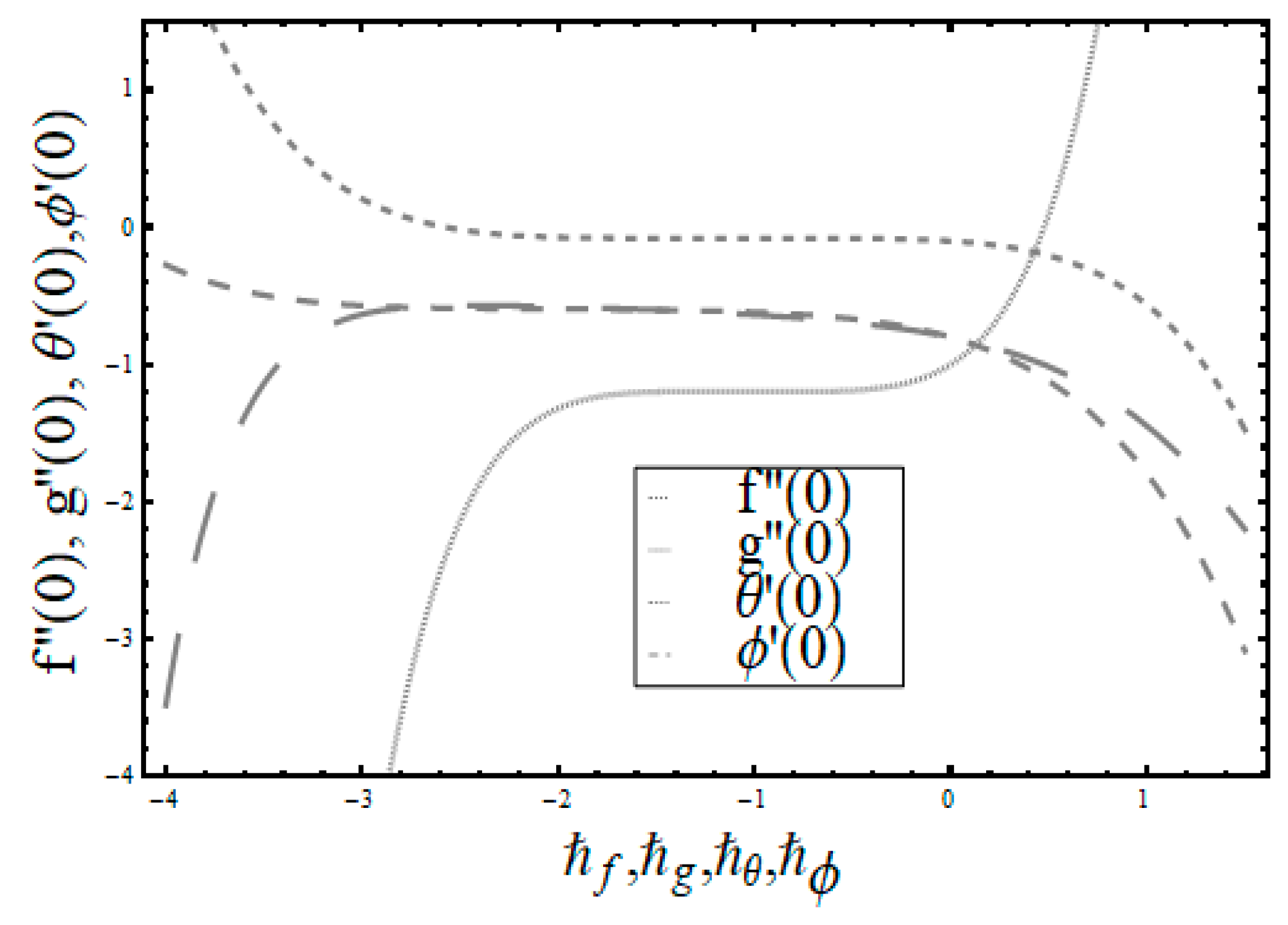
6. Convergence Analysis

HAM is used to obtain the solution of higher order nonlinear problems or those in series form. It gives several choices to control and modify the convergence region for the series solutions. Figure 2 represents the $\hslash -$ curves behavior of all distributions. Characteristic parameters ${\hslash }_f,{\hslash }_g,{\hslash }_{\theta }$ and ${\hslash }_{\varphi }$ have permissible ranges $-1.6\le {\hslash }_f\le -0.4,-2.15\le {\hslash }_g\le -0.2,-2.75\le {\hslash }_{\theta }\le -0.8$ and $-2.6\le {\hslash }_{\varphi }\le -0.6$ when γ = 0.2, Le = 1, $N_t$ = 0.2, $N_b$ = 0.3, Pr = 1.0, ε = 0.3, λ = 0.002, β₁= β₃ = 0.2, β = 0.1 and M = 0.2

Table 1. Convergence analysis of series solution using different order approximations when M = 0.2, γ₁ =0.2, γ₂ = 0.2, $N_b$ = 0.3, $N_t$ = 0.2, λ = 0.002, Le = 1.0, Pr = 1.0 δ_t = 0.2, δ_c = 0.2, ε =0.1, β = 0.1.

Order of Approximations	$-\mathit{f}″(0)$	$\mathit{g}″(0)$	$-\mathit{\theta }\prime (0)$	$-\mathit{\varphi }\prime (0)$
1	1.13509	0.07226	0.31147	0.53000
5	1.27039	0.07329	0.35690	0.46424
10	1.33592	0.07344	0.36006	0.44888
20	1.37389	0.07360	0.36099	0.44350
25	1.38731	0.07368	0.36158	0.44215
30	1.38731	0.07368	0.36158	0.44215

represents the numerical results obtained for series solutions depicting the convergence of approximations up to the 25th order of approximations, that is, enough for series solution convergence. It can be verified that the graphical depiction in Figure 2 and the tabular results in Table 1 are in total consensus.

Table 2. Comparative estimates of We with Malik et al. [50] for skin friction along both directions in the limiting case, i.e., by considering the Hartmann number, second-order slip, temperature, and concentration profiles to zero.

We	$-{[\mathit{f}″+\frac{\mathit{W}\mathit{e}}{2}{(\mathit{f}″)}^2]}_{\mathit{\eta }=0}$		$-{[\mathbf{g}″+\frac{\mathit{W}\mathit{e}}{2}{(\mathbf{g}″)}^2]}_{\mathit{\eta }=0}$
	[40]	Present Outcomes	[50]	Present Outcomes
0.1	1.0934	1.0933	0.4661	0.4660
0.2	1.2695	1.2695	0.4841	0.4841
0.3	1.3340	1.3341	0.5025	0.5024
0.4	1.4915	1.4916	0.5220	0.5221

was developed to validate the results obtained in the current model for skin friction in both directions by comparison with Malik et al. [50], and excellent harmony in both outcomes is achieved.

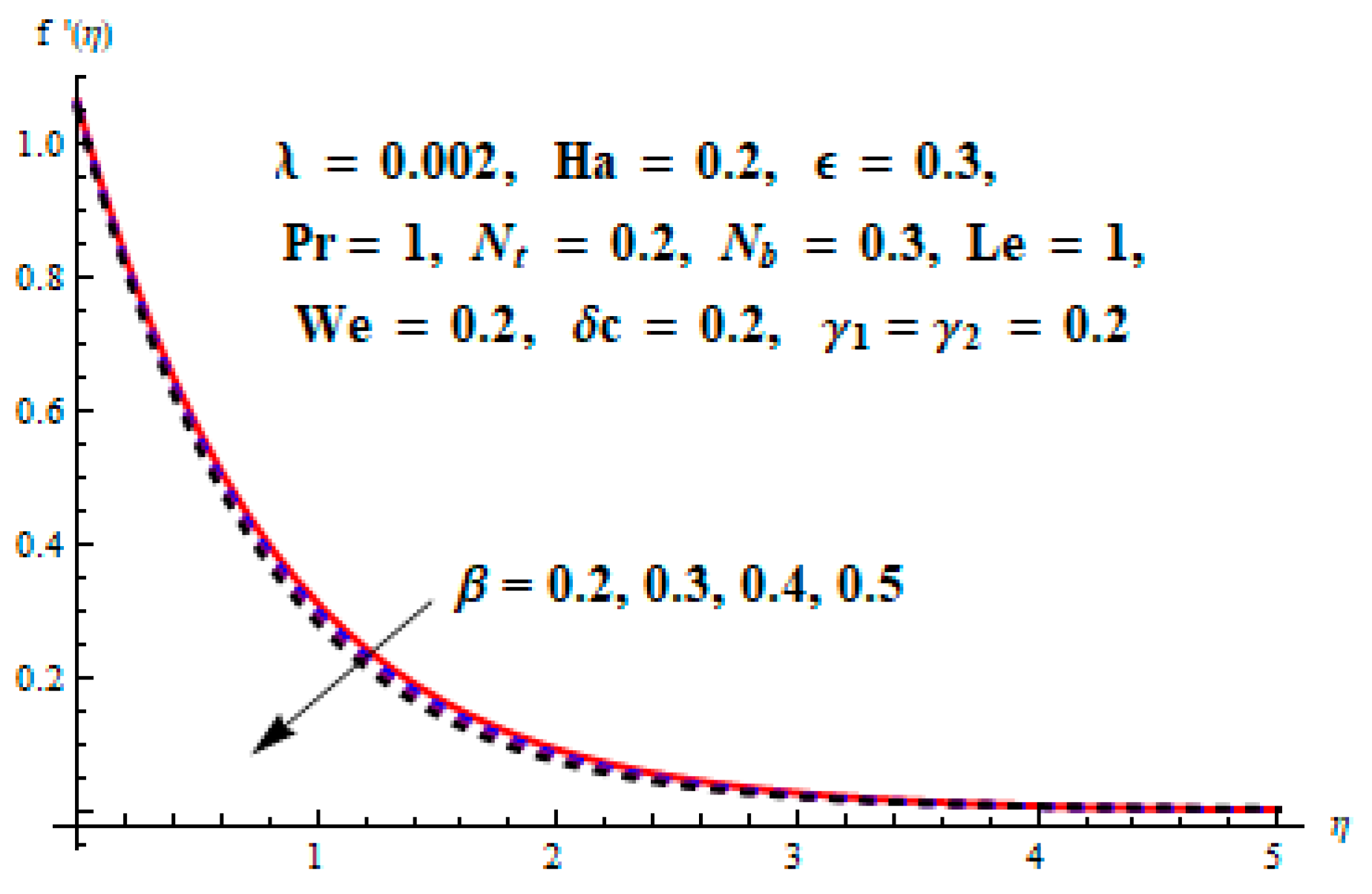
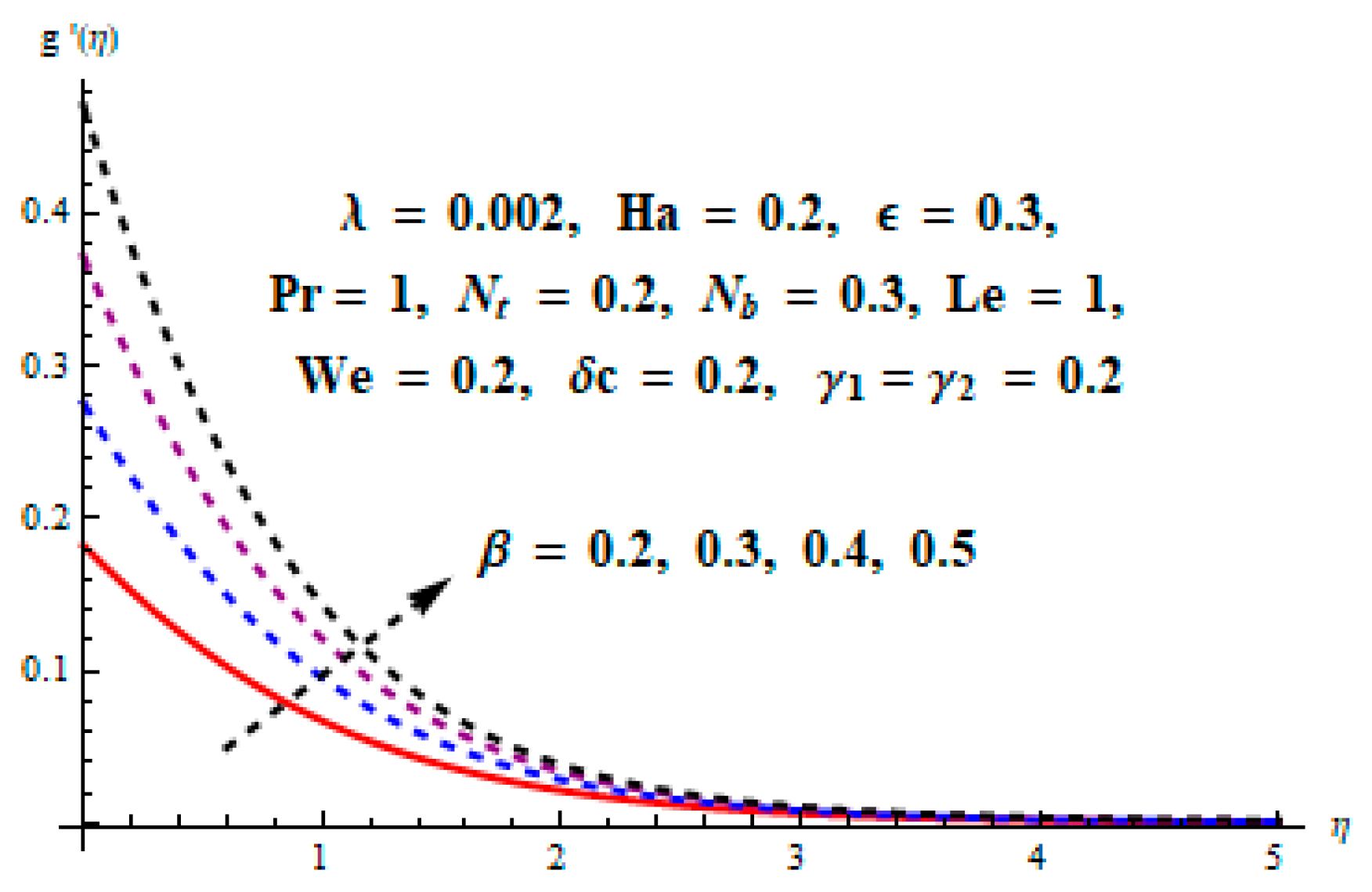
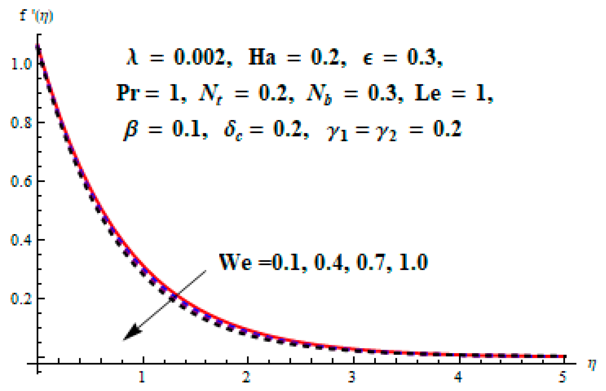
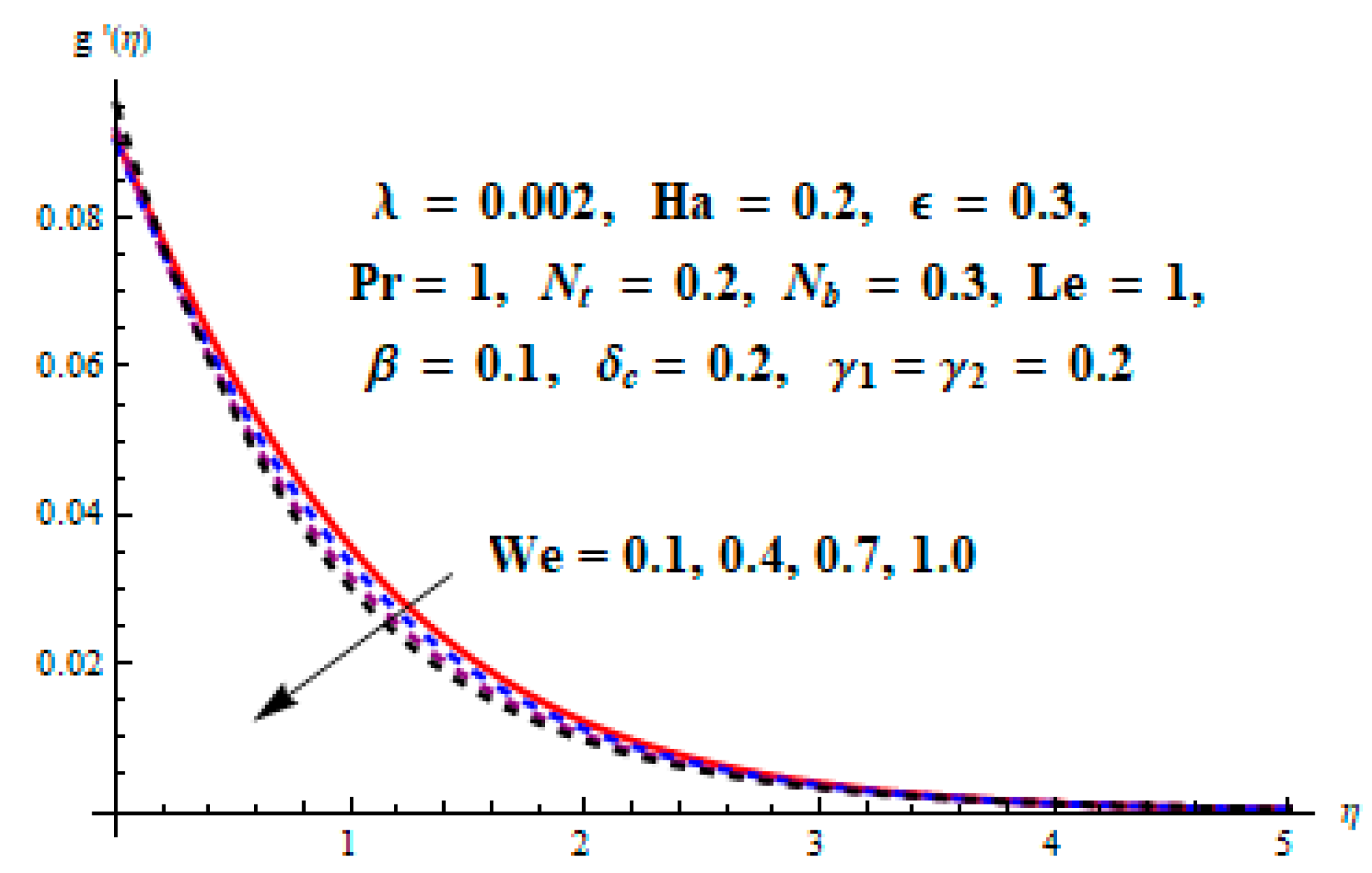
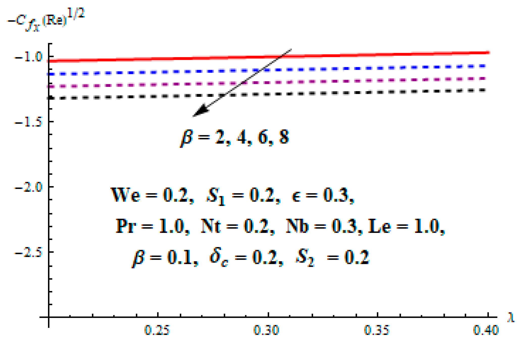
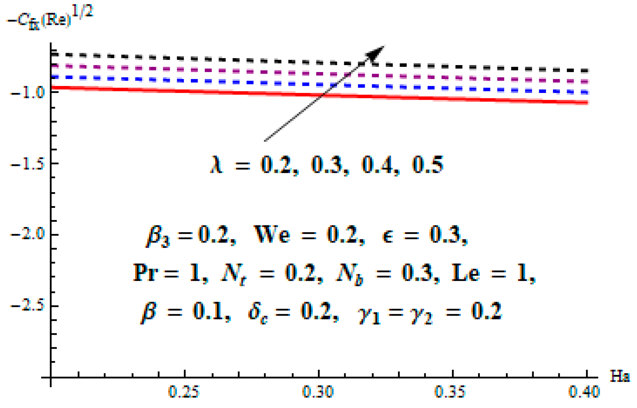
7. Results and Discussion

In this section, we analyze the impact of appearing factors on particular distributions in Figure 3, Figure 4, Figure 5, Figure 6, Figure 7, Figure 8, Figure 9, Figure 10, Figure 11, Figure 12, Figure 13, Figure 14, Figure 15, Figure 16, Figure 17, Figure 18, Figure 19, Figure 20 and Figure 21. The behavior on velocity profiles of $\beta$ (ratio parameter) is described in Figure 3 and Figure 4. It is noticed that contradictory behavior shown by both velocities ($f\prime$, $g\prime$) for an increasing rate of $\beta$. As $\beta =\frac{b}{a}$, $a$ was smaller for higher values of $\beta$, which specified a decreasing velocity rate along the x-direction, or $b$ with higher values specified an increasing rate along the y-direction. In Figure 5 and Figure 6, ${\delta }_t\mathrm{and}{\delta }_c$ illustrate the influence of thermal relaxation and the concentration relaxation factor on temperature concentration and distributions. We found that both concentration and temperature fields associated with the thickness of the boundary layers were the functions of decreasing ${\delta }_c$ and ${\delta }_t$, respectively. Furthermore, ${\delta }_c=0$ and ${\delta }_t=0$ existing model will transform into classical laws of Fick’s and Fourier’s respectively. The influence of thermal conductivity $\epsilon$ on the temperature distribution is described in Figure 7. For higher values of $\epsilon$, an increasing rate for the thermal boundary layer is found, which in result increases the temperature distribution. In Figure 8 the impact of Lewis number Le on concentration field is described. The strength of Lewis number depends on smaller estimations of mass diffusivity than the thermal diffusivity, which shows that exhausted Brownian motion coefficient decreases nanoparticle concentration profile. Figure 9 highlighted the influence of mixed convective factor $\lambda$ on the velocity field ($g\prime$). Higher estimations of $\lambda$ produce stronger buoyancy force, which indicates an increasing rate in the velocity field ($g\prime$). The behavior of Prandtl number Pr against temperature distribution is presented in Figure 10. It is inspected that heat diffusion is very slow from the heated surface for higher estimates of Pr than smaller estimations of Pr. Therefore, temperature decreases with increasing values of Pr. Figure 11 and Figure 12 show the influence of Ha (Hartmann number) on both velocity profiles ($f\prime$,$g\prime$). Retardation in the fluid motion is seen due to resistance effered by strong Lorentz force. This act finally points out the decreasing rate on both velocity distributions. Figure 13 and Figure 14 demonstrate the impact of Brownian motion factor $N_b$ on concentration and temperature distribution. For the larger estimates of $N_b$, fluid temperature increases and rapidly reduces the deposition of particles far away from the fluid on the stretched surface. Due to which it increases and decreases concentration. The influence of the $N_t$ on the concentration distribution is described in Figure 15. When the estimates of $N_t$ are high and they are directly proportional to the temperature distribution, as a result it enhances the concentration distribution and its concentration associated with thickness of boundary layer. Figure 16 illustrates the influence of $N_t$ on the temperature profile. When the values of $N_t$ are higher, nanoparticles move from ambient fluid with higher temperature to the ambient fluid with lower temperature, and as a results temperature is higher in the boundary layer region. Finally, we identified the thickness of augmented thermal boundary layer. Figure 17 and Figure 18 are drawn to display the influence of Williamson fluid parameter We on both velocity profiles. Increasing values of We decrease both velocities profiles. By increasing Williamson factor, relaxation time enhances. It causes to increase liquid viscosity, which results in decrease in the velocity profile. In Figure 19 the impact of stretching ratio factor $\beta$ and mixed convective parameter $\lambda$ on coefficient of Skin friction along $x$-direction is displayed. Which highlighted that the coefficient of Skin friction shpws increasing behavior versus $\beta$ and $\lambda$. Similar tendency can be observed in Hartmann number $Ha$ and mixed convective parameter λ, against coefficient of Skin friction in $x$-direction, as displayed in Figure 20. Analysis of the impact of $\lambda$ and Nr on Skin friction is described in Figure 21. It is noted that a thinner boundary layer is associated with larger $\lambda$, which result in higher velocity gradient near the wall. That’s why Skin friction reduces against $\lambda$.

8. Concluding Remarks

Three-dimensional Williamson nanofluid flow was investigated considering the Cattaneo–Christov heat flux model. The originality of the envisioned mathematical model was boosted by considering the influence of double stratification and second-order slip. HAM was applied to obtain the problem solution in series form. The salient outcomes of the problem are as follows:

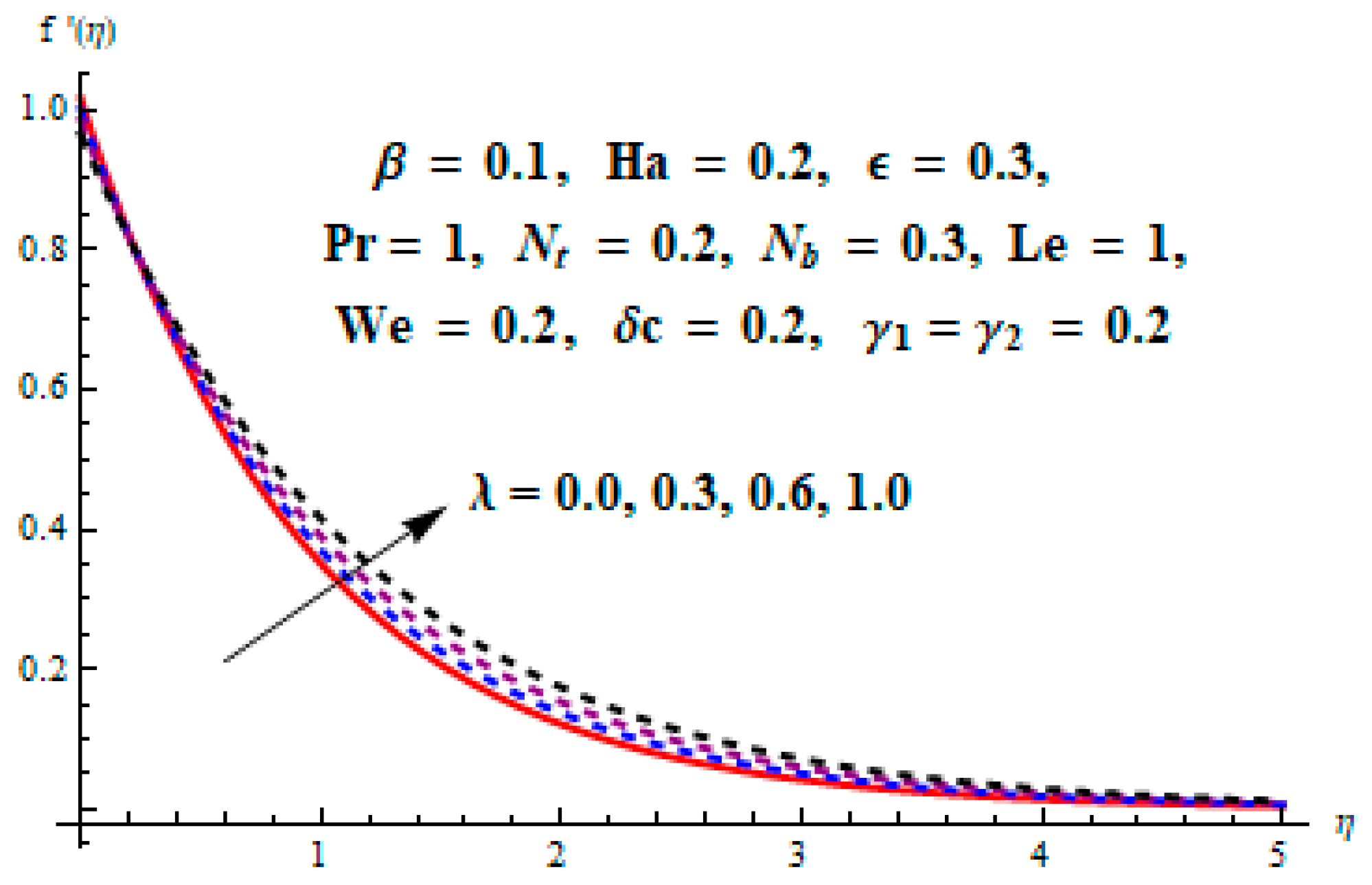
• The stretching ratio parameter had an opposite impact on both velocities.
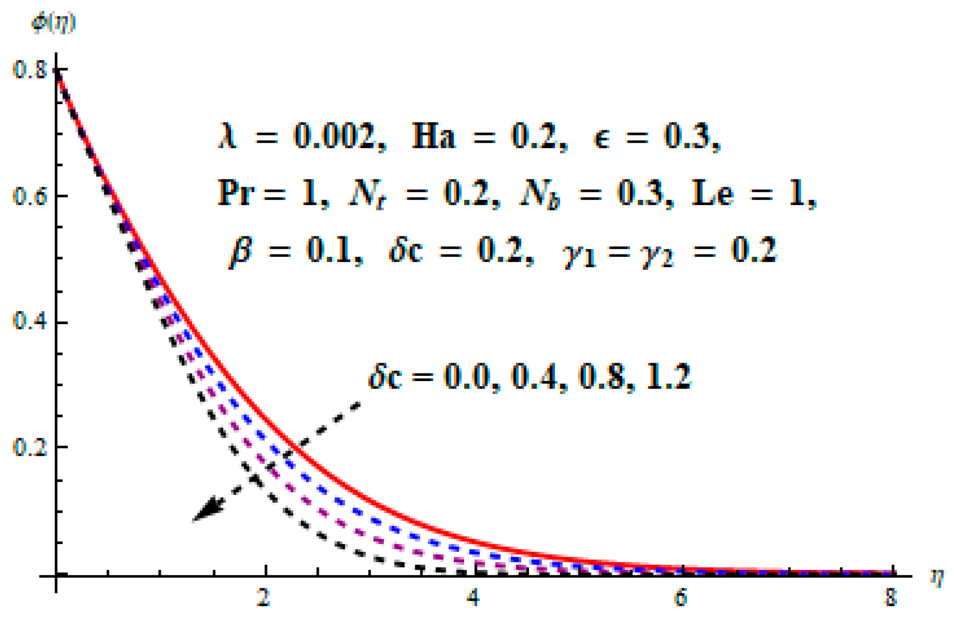
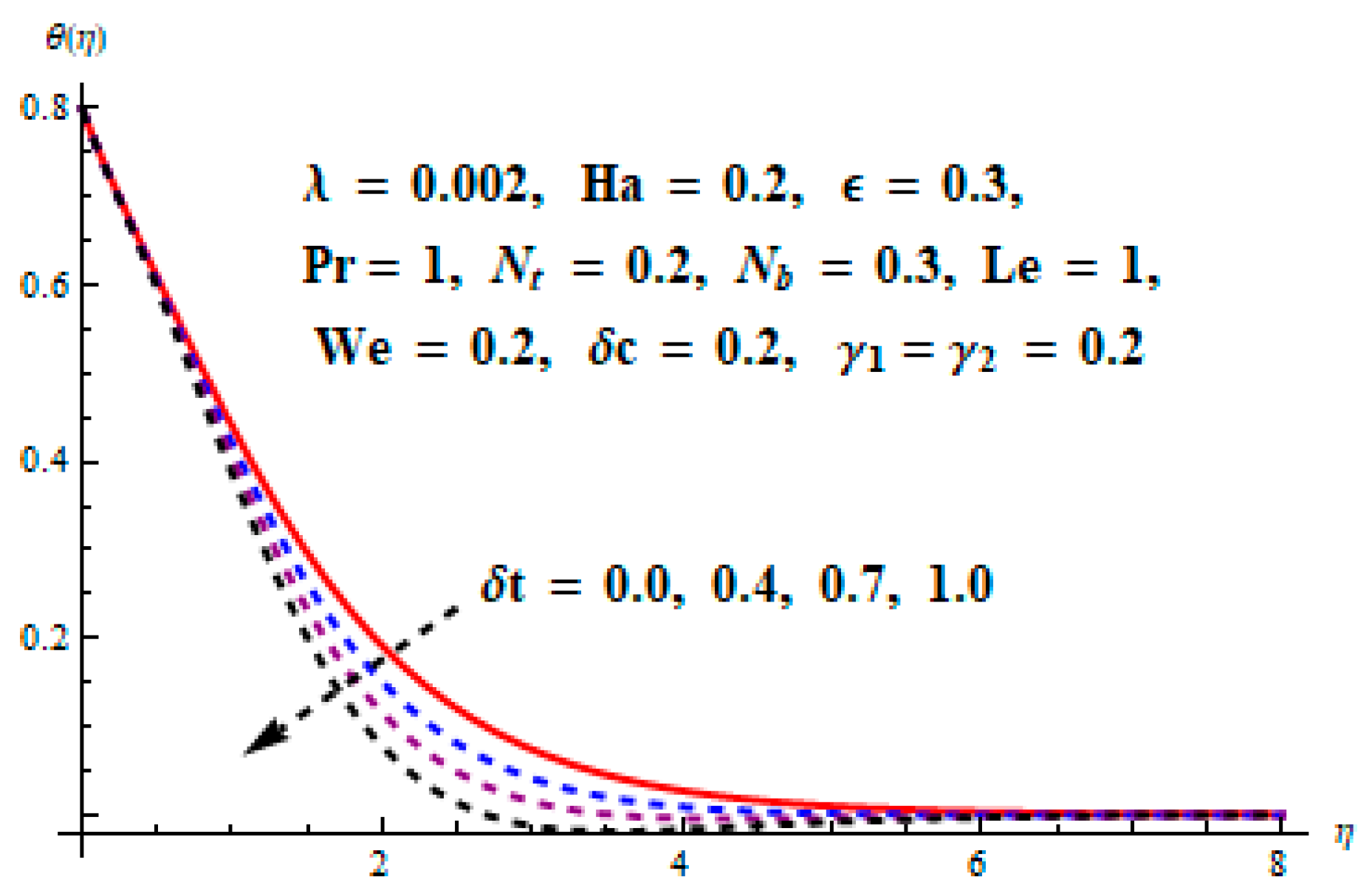
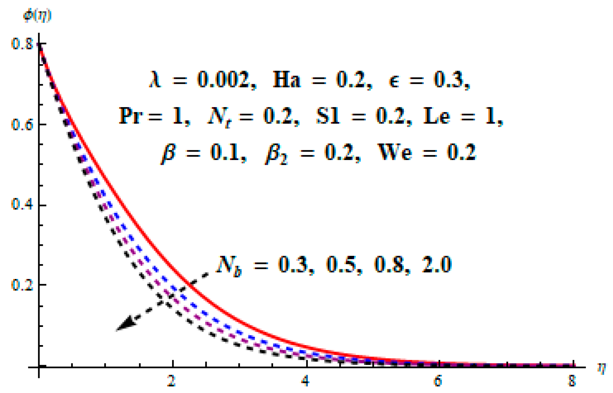
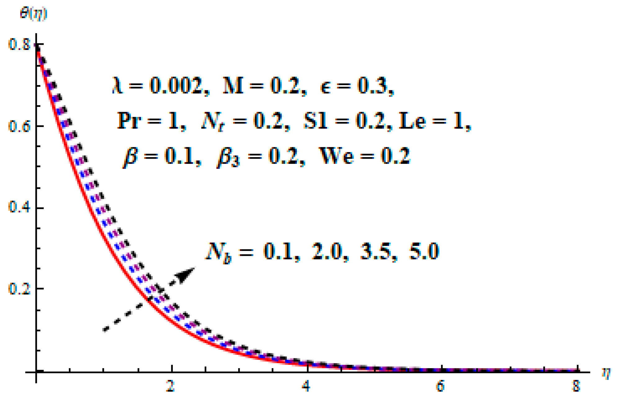
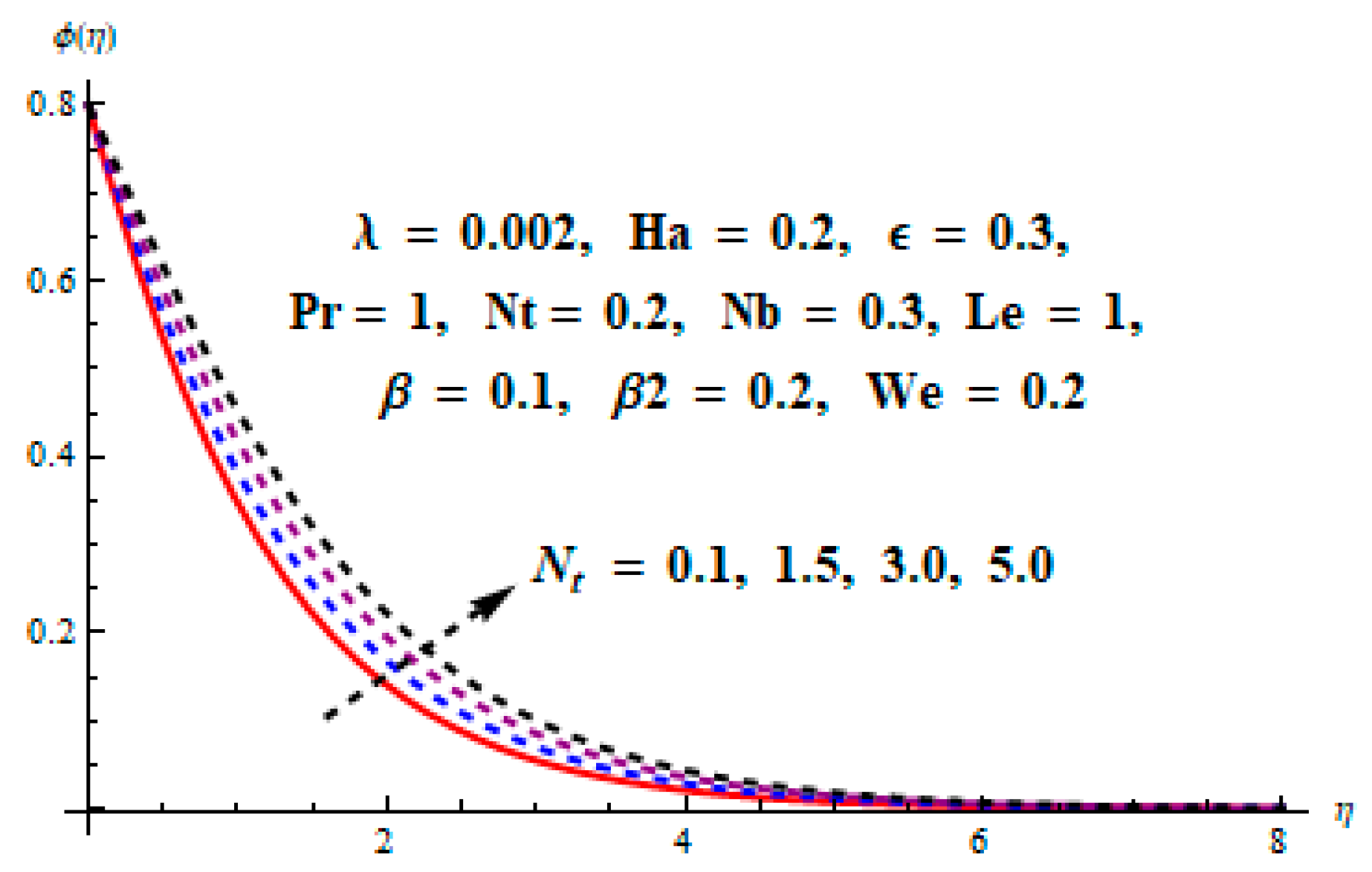
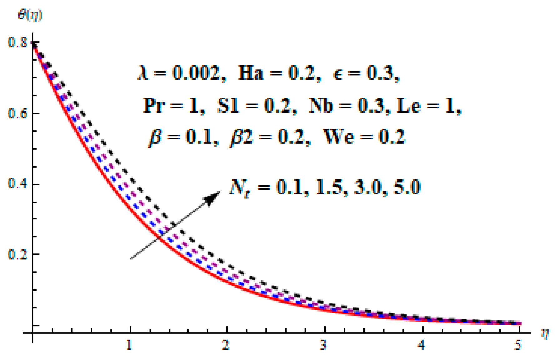
• Increasing values of concentrations and temperature distributions decreased the thermal and concentration relaxation parameters, respectively.
• The higher temperature was in direct proportion with the thermal conductivity parameter.
• Velocity increased for values of the mixed convection parameter.
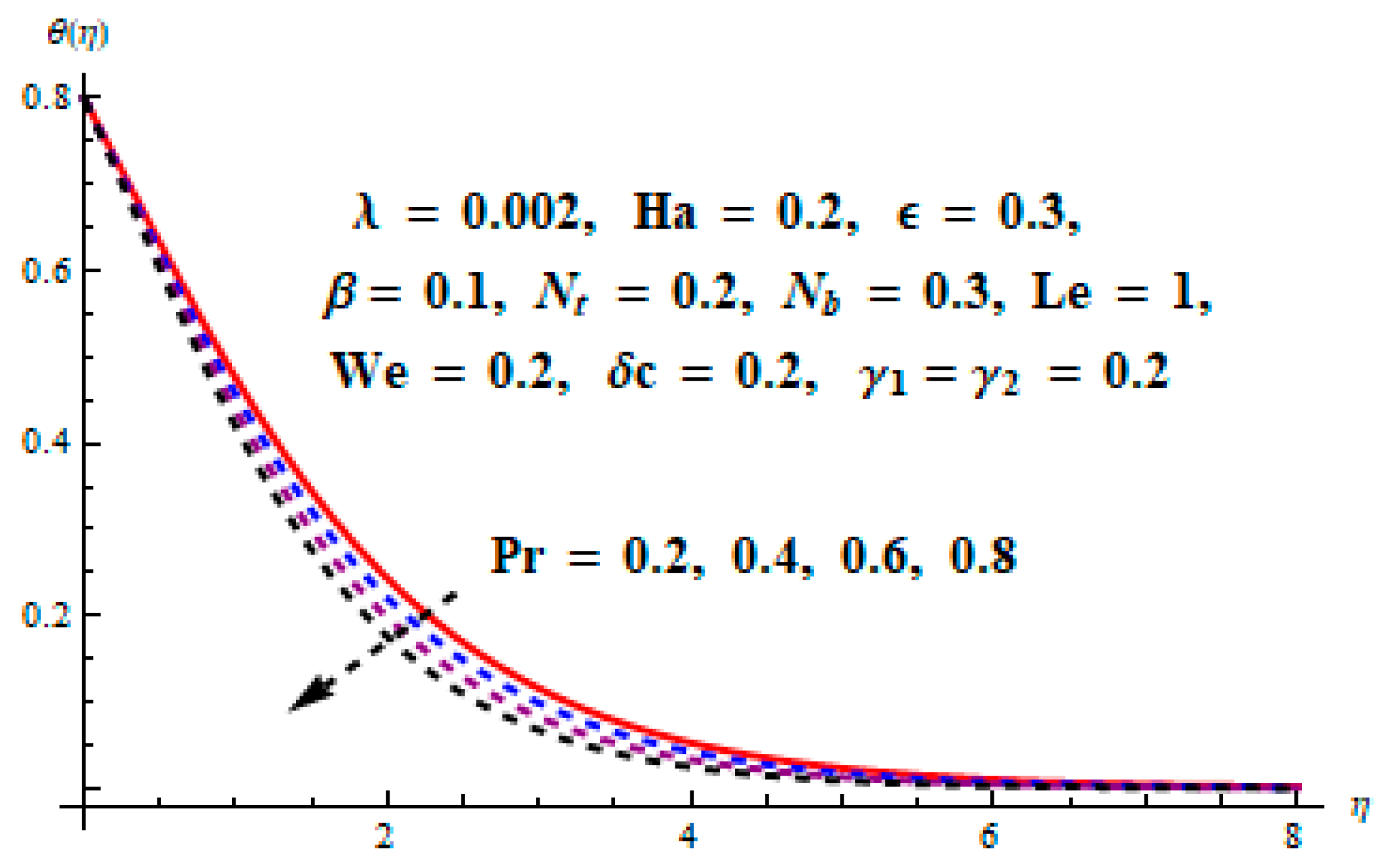
• For the large values of the Prandtl number, fluid temperature decreased.
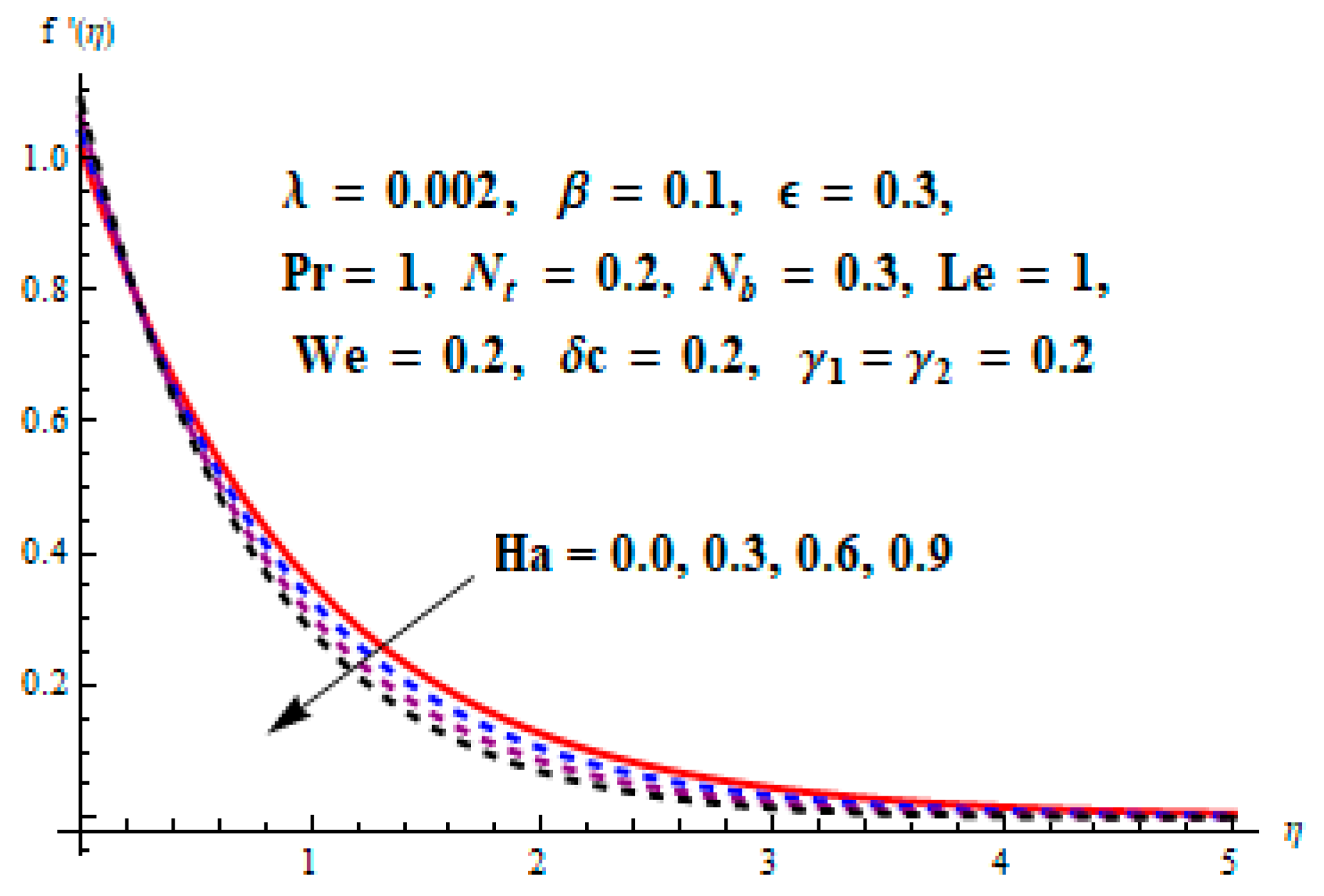
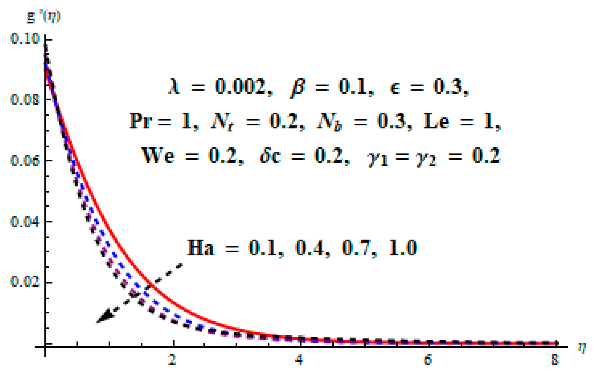
• Both velocity components were decreasing functions of the Hartmann number.
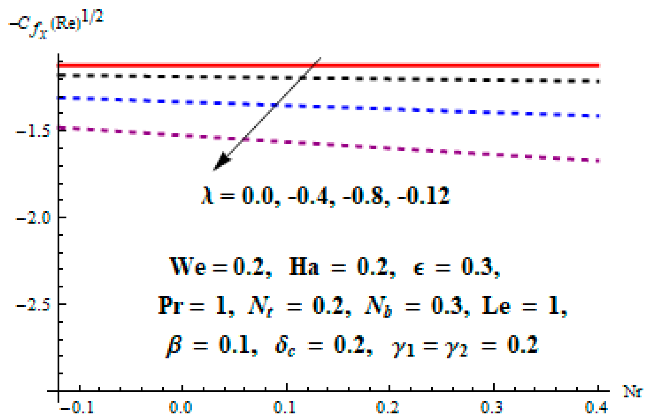
• Skin friction coefficients against the x- and y- directions displayed an accelerating tendency with respect to values of the stretching ratio and mixed convection parameters.

References

1. Straughan, B. Thermal convection with the Cattaneo–Christov model. Int. J. Heat Mass Transf. 2010, 53, 95–98. [Google Scholar] [CrossRef]
2. Khan, W.A.; Khan, M.; Alshomrani, A.S.; Ahmad, L. Numerical investigation of generalized Fourier’s and Fick’s laws for Sisko fluid flow. J. Mol. Liq. 2016, 224, 1016–1021. [Google Scholar] [CrossRef]
3. Hayat, T.; Khan, M.I.; Farooq, M.; Alsaedi, A.; Waqas, M.; Yasmeen, T. Impact of Cattaneo–Christov heat flux model inflow of variable thermal conductivity fluid over a variable thicked surface. Int. J. Heat Mass Transf. 2016, 99, 702–710. [Google Scholar] [CrossRef]
4. Waqas, M.; Hayat, T.; Farooq, M.; Shehzad, S.A.; Alsaedi, A. Cattaneo-Christov heat flux model for the flow of variable thermal conductivity generalized Burgers fluid. Int. J. Heat Mass Transf. 2016, 220, 642–648. [Google Scholar] [CrossRef]
5. Khan, A.U.; Ahmed, N.; Mohyud-Din, S.T. Thermo-diffusion and diffusion-thermo effects on the flow of second-grade fluid between two inclined plane walls. J. Mol. Liq. 2016, 224, 1074–1082. [Google Scholar]
6. Ghadikolaei, S.S.; Hosseinzadeh, K.; Yassari, M.; Sadeghi, H.; Ganji, D.D. Analytical and numerical solution of non-Newtonian second-grade fluid flow on a stretching sheet. Therm. Sci. Eng. Prog. 2018, 5, 309–316. [Google Scholar] [CrossRef]
7. Khan, I.; Malik, M.Y.; Salahuddin, T.; Khan, M.; Rehman, K.U. Homogenous–heterogeneous reactions in MHD flow of Powell–Eyring fluid over a stretching sheet with Newtonian heating. Neural Comput. Appl. 2018, 30, 3581–3588. [Google Scholar] [CrossRef] [Green Version]
8. Ibrahim, W.; Shankar, B.; Nandeppanavar, M.M. MHD stagnation point flow and heat transfer due to nanofluid towards a stretching sheet. Int. J. Heat Mass Transf. 2013, 56, 1–9. [Google Scholar] [CrossRef]
9. Chamkha, A.J.; Al-Mudhaf, A. Unsteady heat and mass transfer from a rotating vertical cone with a magnetic field and heat generation or absorption effects. Int. J. Therm. Sci. 2005, 44, 267–276. [Google Scholar] [CrossRef]
10. Pullepu, B.; Chamkha, A.J.; Pop, I. Unsteady laminar free convection flows past a non-isothermal vertical cone in the presence of a magnetic field. Chem. Eng. Commun. 2012, 199, 354–367. [Google Scholar] [CrossRef]
11. Akbar, N.S.; Nadeem, S.; Haq, R.U.; Khan, Z.H. Numerical solutions of Magnetohydrodynamic boundary layer flow of tangent hyperbolic fluid towards a stretching sheet. Indian J. Phys. 2013, 87, 1121–1124. [Google Scholar] [CrossRef]
12. Seini, I.Y.; Makinde, O.D. Boundary layer flow near stagnation-points on a vertical surface with a slip in the presence of the transverse magnetic field. Int. J. Numer. Methods Heat Fluid Flow 2014, 24, 643–653. [Google Scholar] [CrossRef]
13. Ravindran, R.; Ganapathirao, M.; Pop, I. Effects of chemical reaction and heat generation/absorption on unsteady mixed convection MHD flow over a vertical cone with non-uniform slot mass transfer. Int. J. Heat Mass Transf. 2014, 73, 743–751. [Google Scholar] [CrossRef]
14. Bovand, M.; Rashidi, S.; Esfahani, J.A.; Saha, S.C.; Gu, Y.T.; Dehesht, M. Control of flow around a circular cylinder wrapped with a porous layer by magnetohydrodynamic. J. Magn. Magn. Mater. 2016, 401, 1078–1087. [Google Scholar] [CrossRef]
15. Ellahi, R.; Bhatti, M.M.; Pop, I. Effects of the hall and ion slip on MHD peristaltic flow of Jeffrey fluid in a non-uniform rectangular duct. Int. J. Numer. Methods Heat Fluid Flow 2016, 26, 1802–1820. [Google Scholar] [CrossRef]
16. Mishra, S.R.; Pattnaik, P.K.; Bhatti, M.M.; Abbas, T. Analysis of heat and mass transfer with MHD and chemical reaction effects on viscoelastic fluid over a stretching sheet. Indian J. Phys. 2017, 91, 1219–1227. [Google Scholar] [CrossRef]
17. Hussain, A.; Malik, M.Y.; Awais, M.; Salahuddin, T.; Bilal, S. Computational and physical aspects of MHD Prandtl-Eyring fluid flow analysis over a stretching sheet. Neural Comput. Appl. 2019, 31, 425–433. [Google Scholar] [CrossRef]
18. Khan, W.A.; Pop, I. Boundary-layer flow of a nanofluid past a stretching sheet. Int. J. Heat Mass Transf. 2010, 53, 2477–2483. [Google Scholar] [CrossRef]
19. Makinde, O.D.; Aziz, A. Boundary layer flow of a nanofluid past a stretching sheet with a convective boundary condition. Int. J. Therm. Sci. 2011, 50, 1326–1332. [Google Scholar] [CrossRef]
20. Nadeem, S.; Mehmood, R.; Akbar, N.S. Non-orthogonal stagnation point flow of a nano non-Newtonian fluid towards a stretching surface with heat transfer. Int. J. Heat Mass Transf. 2013, 57, 679–689. [Google Scholar] [CrossRef]
21. Hatami, M.; Jing, D.; Song, D.; Sheikholeslami, M.; Ganji, D.D. Heat transfer and flow analysis of nanofluid flow between parallel plates in the presence of a variable magnetic field using HPM. J. Magn. Magn. Mater. 2015, 396, 275–282. [Google Scholar] [CrossRef]
22. Hayat, T.; Imtiaz, M.; Alsaedi, A. MHD 3D flow of a nanofluid in the presence of convective conditions. J. Mol. Liq. 2015, 212, 203–208. [Google Scholar] [CrossRef]
23. Sheikholeslami, M.; Ganji, D.D.; Javed, M.Y.; Ellahi, R. Effect of thermal radiation on magnetohydrodynamics nanofluid flow and heat transfer by means of a two-phase model. J. Magn. Magn. Mater. 2015, 374, 36–43. [Google Scholar] [CrossRef]
24. Sheikholeslami, M.; Rokni, H.B. Nanofluid two-phase model analysis in the existence of induced magnetic field. Int. J. Heat Mass Trans. 2017, 107, 288–299. [Google Scholar] [CrossRef]
25. Hassan, M.; Marin, M.; Alsharif, A.; Ellahi, R. Convective heat transfer flow of a nanofluid in a porous medium over wavy surface. Phys. Lett. A 2018, 382, 2749–2753. [Google Scholar] [CrossRef]
26. Nayak, M.K.; Shaw, S.; Pandey, V.S.; Chamkha, A.J. Combined effects of slip and convective boundary condition on MHD 3D stretched flow of nanofluid through porous media inspired by non-linear thermal radiation. Indian J. Phys. 2018, 92, 1–12. [Google Scholar] [CrossRef]
27. Hosseini, S.R.; Sheikholeslami, M.; Ghasemian, M.; Ganji, D.D. Nanofluid heat transfer analysis in a microchannel heat sink (MCHS) under the effect of a magnetic field by means of the KKL model. Powder Technol. 2018, 324, 36–47. [Google Scholar] [CrossRef]
28. Lu, D.; Ramzan, M.; Mohammad, M.; Howari, F.; Chung, J.D. A Thin Film Flow of Nanofluid Comprising Carbon Nanotubes Influenced by Cattaneo-Christov Heat Flux and Entropy Generation. Coatings 2019, 9, 296. [Google Scholar] [CrossRef] [Green Version]
29. Li, Z.; Shafee, A.; Ramzan, M.; Rokni, H.B.; Al-Mdallal, Q.M. Simulation of natural convection of Fe 3 O 4-water ferrofluid in a circular porous cavity in the presence of a magnetic field. Eur. Phys. J. Plus 2019, 134, 77. [Google Scholar] [CrossRef]
30. Suleman, M.; Ramzan, M.; Ahmad, S.; Lu, D.; Muhammad, T.; Chung, J.D. A Numerical Simulation of Silver–Water Nanofluid Flow with Impacts of Newtonian Heating and Homogeneous–Heterogeneous Reactions Past a Nonlinear Stretched Cylinder. Symmetry 2019, 11, 295. [Google Scholar] [CrossRef] [Green Version]
31. Lu, D.; Li, Z.; Ramzan, M.; Shafee, A.; Chung, J.D. Unsteady squeezing carbon nanotubes based nano-liquid flow with Cattaneo–Christov heat flux and homogeneous–heterogeneous reactions. Appl. Nanosci. 2019, 9, 169–178. [Google Scholar] [CrossRef]
32. Ramzan, M.; Sheikholeslami, M.; Saeed, M.; Chung, J.D. On the convective heat and zero nanoparticle mass flux conditions in the flow of 3D MHD Couple Stress nanofluid over an exponentially stretched surface. Sci. Rep. 2019, 9, 562. [Google Scholar] [CrossRef] [PubMed] [Green Version]
33. Li, Z.; Sheikholeslami, M.; Shafee, A.; Ramzan, M.; Kandasamy, R.; Al-Mdallal, Q.M. Influence of adding nanoparticles on solidification in a heat storage system considering radiation effect. J. Mol. Liq. 2019, 273, 589–605. [Google Scholar] [CrossRef]
34. Farooq, U.; Lu, D.C.; Munir, S.; Suleman, M.; Ramzan, M. Flow of Rheological Nanofluid over a Static Wedge. J. Nanofluids 2019, 8, 1362–1366. [Google Scholar] [CrossRef]
35. Qayyum, S.; Khan, M.I.; Hayat, T.; Alsaedi, A. Comparative investigation of five nanoparticles in flow of viscous fluid with Joule heating and slip due to rotating disk. Phys. B Condens. Matter 2018, 534, 173–183. [Google Scholar] [CrossRef]
36. Nguyen, T.; van der Meer, D.; van den Berg, A.; Eijkel, J.C. Investigation of the effects of time periodic pressure and potential gradients on viscoelastic fluid flow in circular narrow confinements. Microfluid. Nanofluid. 2017, 21, 37. [Google Scholar] [CrossRef] [Green Version]
37. Ramzan, M.; Bilal, M.; Chung, J.D. Radiative Williamson nanofluid flow over a convectively heated Riga plate with chemical reaction-A numerical approach. Chin. J. Phys. 2017, 55, 1663–1673. [Google Scholar] [CrossRef]
38. Ramzan, M.; Bilal, M.; Chung, J.D. MHD stagnation point Cattaneo–Christov heat flux in Williamson fluid flow with homogeneous–heterogeneous reactions and convective boundary condition—A numerical approach. J. Mol. Liq. 2017, 225, 856–862. [Google Scholar] [CrossRef]
39. Nadeem, S.; Hussain, S.T. Flow and heat transfer analysis of Williamson nanofluid. Appl. Nanosci. 2014, 4, 1005–1012. [Google Scholar] [CrossRef] [Green Version]
40. Nadeem, S.; Maraj, E.N.; Akbar, N.S. Investigation of peristaltic flow of Williamson nanofluid in a curved channel with compliant walls. Appl. Nanosci. 2014, 4, 511–521. [Google Scholar] [CrossRef] [Green Version]
41. Liao, S.J. Beyond Perturbation; Chapman & Hall/CRC Press: Boca Raton, FL, USA, 2003. [Google Scholar]
42. Jafarimoghaddam, A. On the Homotopy Analysis Method (HAM) and Homotopy Perturbation Method (HPM) for a nonlinearly stretching sheet flow of Eyring-Powell fluids. Eng. Sci. Technol. Int. J. 2019, 22, 439–451. [Google Scholar] [CrossRef]
43. Freidoonimehr, N.; Rostami, B.; Rashidi, M.M. Predictor homotopy analysis method for nanofluid flow through expanding or contracting gaps with permeable walls. Int. J. Biomath. 2015, 8, 1550050. [Google Scholar] [CrossRef]
44. Ray, A.K.; Vasu, B.; Bég, O.A.; Gorla, R.S.; Murthy, P.V.S.N. Homotopy semi-numerical modeling of non-Newtonian nanofluid transport external to multiple geometries using a revised Buongiorno Model. Inventions 2019, 4, 54. [Google Scholar] [CrossRef] [Green Version]
45. Shukla, N.; Rana, P.; Bég, O.A.; Singh, B.; Kadir, A. Homotopy study of magnetohydrodynamic mixed convection nanofluid multiple slip flow and heat transfer from a vertical cylinder with entropy generation. Propuls. Power Res. 2019, 8, 147–162. [Google Scholar] [CrossRef]
46. Shqair, M. Solution of different geometries reflected reactors neutron diffusion equation using the homotopy perturbation method. Results Phys. 2019, 12, 61–66. [Google Scholar] [CrossRef]
47. Ramzan, M.; Farooq, M.; Alsaedi, A.; Hayat, T. MHD three-dimensional flow of couple stress fluid with Newtonian heating. Eur. Phys. J. Plus 2013, 128, 49. [Google Scholar] [CrossRef]
48. Hussain, T.; Shehzad, S.A.; Hayat, T.; Alsaedi, A.; Al-Solamy, F.; Ramzan, M. Radiative hydromagnetic flow of Jeffrey nanofluid by an exponentially stretching sheet. PLoS ONE 2014, 9, e103719. [Google Scholar] [CrossRef]
49. Ramzan, M.; Yousaf, F. Boundary layer flow of three-dimensional viscoelastic nanofluid past a bi-directional stretching sheet with Newtonian heating. AIP Adv. 2015, 5, 057132. [Google Scholar] [CrossRef]
50. Malik, M.Y.; Bilal, S.; Salahuddin, T.; Rehman, K.U. Three-dimensional Williamson fluid flow over a linearly stretching surface. Math. Sci. Lett. 2017, 6, 53–61. [Google Scholar] [CrossRef]
Figure 1. Schematic flow diagram.
Coatings 09 00849 g001
Figure 2. curves for f , g , θ    and ϕ .
Coatings 09 00849 g002
Figure 3. Impact of β against f’.
Coatings 09 00849 g003
Figure 4. Impact of β against g’.
Coatings 09 00849 g004
Figure 5. Impact of δc against ϕ.
Coatings 09 00849 g005
Figure 6. Impact of δt against θ.
Coatings 09 00849 g006
Figure 7. Impact of ∈ against θ.
Coatings 09 00849 g007
Figure 8. Impact of Le against ϕ.
Coatings 09 00849 g008
Figure 9. Impact of λ against f’.
Coatings 09 00849 g009
Figure 10. Impact of Pr against θ.
Coatings 09 00849 g010
Figure 11. Impact of H a against f’.
Coatings 09 00849 g011
Figure 12. Impact of H a against g’.
Coatings 09 00849 g012
Figure 13. Impact of Nb against ϕ.
Coatings 09 00849 g013
Figure 14. Impact of Nb against θ.
Coatings 09 00849 g014
Figure 15. Impact of Nt against ϕ.
Coatings 09 00849 g015
Figure 16. Impact of Nt against θ.
Coatings 09 00849 g016
Figure 17. Impact of We against f’.
Coatings 09 00849 g017
Figure 18. Impact of We against g’.
Coatings 09 00849 g018
Figure 19. Impact of λ and β against Skin friction.
Coatings 09 00849 g019
Figure 20. Impact of λ and H a against Skin friction.
Coatings 09 00849 g020
Figure 21. Impact of Nr and λ against Skin friction.
Coatings 09 00849 g021