Article

Impact of Velocity Second Slip and Inclined Magnetic Field on Peristaltic Flow Coating with Jeffrey Fluid in Tapered Channel

1
College of Sciences and Human Studies, Prince Mohammad Bin Fahd University, Alkhobar 31952, Saudi Arabia
2
MCS, National University of Sciences and Technology, Islamabad, Pakistan
3
Department of Mathematics, Faculty of Science, University of Jeddah, Jeddah 21598, Saudi Arabia
4
Department of Mathematics, Faculty of Education, Ain Shams University, Roxy 11757, Cairo, Egypt
5
DBS&H CEME, National University of Sciences and Technology, Islamabad, Pakistan
*
Author to whom correspondence should be addressed.
Coatings 2020, 10(1), 30; https://doi.org/10.3390/coatings10010030
Submission received: 28 October 2019 / Revised: 26 November 2019 / Accepted: 17 December 2019 / Published: 1 January 2020
(This article belongs to the Special Issue Recent Trends in Coatings and Thin Film–Modeling and Application)

Abstract

:
The peristaltic flow of velocity second slip boundary conditions and inclined magnetic field of Jeffrey fluid by means of heat and mass transfer in asymmetric channel was inspected in the present study. Leading equations described the existing flow were then simplified under lubrication approach. Therefore, exact solutions of stream function, concentration and temperature were deduced. Further, the numerical solutions of pressure rise and pressure gradient were computed using Mathematica software. Furthermore, the effect of the second slip parameter was argued via graphs. It has been depicted that this kind of slip is mandatory and very imperative to foresee the physical model. On the other hand, false results will be obtained.

1. Introduction

The peristaltic motion induced by channel or tube boundaries has a main role of fluid transport in living organisms and industrial pumping. Additionally, it has attracted attention in the fields of engineering and physiology. This transport is a means of fluid flow in an elastic path by the processes of contraction and expansion. In particular, such flows of viscous and non-Newtonian fluids are widely familiar in several biological systems including the human body in the transport of urine from the kidney to the bladder; chyme movement in the gastrointestinal tract, bile ducts, ureter, esophagus; spermatozoa in ducts efferent of the male reproductive tract; blood circulation in blood vessels; and movement of ovum in female fallopian tubes. Technical roller and finger pumps also function under this type of mechanism. In addition, with the existing of heat transfer, peristalsis is imperative in many processes such as oxygenation and hemodialysis. Further, heat transfer is also noteworthy in the treatment of diseased tissues in cancer. The cram of magnetohy drodynamic (MHD) peristaltic flow is useful as it is used in the reduction of bleeding during surgeries, targeted transfer of drugs via magnetic particles as drug carries, and MRI (magnetic resonance imaging) to diagnose diseases. It also has a pivotal role in the motion of physiological fluids including blood and blood pump machines. Furthermore, mass transfer in peristaltic flow occurs during the chemical breakdown of food, amalgamation of gastric juices with food, diffusive and ionic flows by means of membrane channels, diffusive oxygen transmission in tissue, drug delivery inside the body, and in other digestion processes.
There area lot of models for non-Newtonian fluids due to the complexity of fluids behaviour, like Carreau [1,2,3], Herschel [4,5], Oldroyd [6,7], Williamson [8], Johnson [9,10,11], Casson [12], Couette [13] and further as in [14,15,16,17,18,19,20,21]. Amongst these, the Jeffrey fluid model is considered as the simplest linear model that presents non-Newtonian fluid properties in a way which may enable the researchers to attain exact and analytical solutions. See, for example [22,23,24,25]. Kothandapani and Srinivas [26] have investigated peristaltic transport for Jeffrey fluid under consequences of a magnetic field in an asymmetric channel under the premise of a low Reynolds number and a long wavelength. Tripathi et al. [27] studied MHD peristaltic flow of Jeffrey fluid by means of a finite length cylindrical tube. Further, Nadeem et al. [28] examined the peristaltic flow of MHD Jeffrey fluid in eccentric cylinders. Khan et al. [29] investigated peristaltic transport for Jeffrey fluid with variable viscosity via a porous medium in an asymmetric channel. Srinivas and Pushparaj [30] have presented non-linear peristaltic flow in an inclined asymmetric channel.
In 1827, Navier [31] stated that shear stress at surface is linearly proportional to slip at surface. Fluids revealing slip effects are vital in polishing internal cavities and artificial heart valves. In particular, the application of this condition in peristaltic flows has perfect relevance in the field of polymers and physiology. Studies towards this point of research have been recently taken into account and a wide range of analytical and numerical studies have been reported in [32,33] and [34]. In a porous channel, effects of wall slip conditions and heat transfer on peristaltic transport of MHD Newtonian fluid with elastic wall properties have been discussed by Sirinivas et al. [35]. Hayat et al. [36] introduced a mathematical model in order to study the slip effects of heat and mass transfer on peristaltic transport of MHD power-law fluid and second grade fluid in the channel by flexible walls. Further, Hayat et al. [37] and [38] examined the influence of slip conditions and wall properties in the planar channel on MHD peristaltic flow of Maxwell fluid, and Williamson fluid in the non-uniform channel by heat and mass transfer, respectively. Nadeem and Akram [39] presented effects of partial slip on peristaltic flow of MHD Newtonian fluid in an asymmetric channel. They obtained the solutions using the method of Adomian decomposition and showed that trapping reduces with an increase of the velocity slip parameter, while pressure rise increases with an increase in the slip parameter. Hayat et al. [40,41] have analyzed effects of the slip condition on peristaltic flow of Phan-Thien-Tanner and of an Oldroyd 6-constant fluid, respectively. Mishra and Rao [42] investigated the effects of peristaltic flow of Newtonian fluid in an asymmetric channel. Akram and Nadeem [43] studied consequences with different waveforms of partial slip and nanofluid on peristaltic transport of non-Newtonian fluid. Recently, Hina et al. [44] investigated the peristaltic flow of pseudoplastic fluid with wall properties in a curved channel by heat or mass transfer.
In their important study, Roşca and Pop [45] showed that the second order slip flow model is essential to predict flow characteristics precisely. Very recently, Aly [46,47] and Aly and Vajravelu [48] have studied the effect of second velocity slip on fluid flow. In these studies, it was reported that these type of boundary conditions is compulsory and should be taken into consideration, otherwise, false results will be gained. As mentioned above, there are a considerable number of published papers regarding the effect of the first slip parameter, however, very less consideration has been given to peristaltic flows in the presence of the velocity second slip condition. Recently, Aly and Ebaid [49] presented an exact solution for the outcome of second slip on peristaltic flow of nanofluid in an asymmetric channel.
The intent of the current study is, therefore, to examine the effect of velocity second slip in non-Newtonian fluids by heat and mass transfer in the presence of an inclined magnetic field over an inclined tapered asymmetric channel, as many researchers have recently givenconsiderable attention to this geometry, for example [50,51,52]. As per our knowledge, no effort has been reported yet to discuss this multidimensional analysis, even in the absence of heat and mass transfer; hence, this study may be helpful in this direction of research. The present governing equations for motion, concentration and energy are simplified by assumptions of long wavelength approximation. Then, exact solutions of reduced equations are outlines. Therefore, with help of Mathematica software, many graphical outcomes are plotted and reported for various involved physical parameters of interest.

2. Mathematical Formulation

The peristaltic motion of non-Newtonian incompressible fluid in a vertical tapered asymmetric channel, under effects of a constant magnetic field is considered. It is assumed that a wave train is moving with velocity c along non-uniform walls. In addition, we also assume that the channel andmagnetic field are inclined at angles α and Θ , respectively. Further, upper and lower walls of the channel are sustained at temperature T 0 and T 1 , respectively. For the present flow, U and V are velocities in X and Y directions, respectively, in fixed frame. The upper and lower walls H 1 and H 2 , respectively, of tapered asymmetric channel in fixed frame are defined as:
Y = H 1 = d 1 + k X + a 1 cos [ 2 π λ ( X c t ) ] Y = H 2 = d 2 k X b 1 cos [ 2 π λ ( X c t ) + φ ]
where a 1 and b 1 are amplitudes of waves; λ is wave length; d 1 + d 2 is width of channel; k ( k < < 1 ) is non-uniform parameter; c is velocity of propagation; t is time; phase difference ϕ varies in range 0 φ π ;   φ = 0 corresponds to symmetric channel by waves out of phase and ϕ = π waves are in phase; and further, a 1 , b 1 , d 1 , d 2 and ϕ satisfy the condition [24].
a 1 2 + b 1 2 + 2 a 1 b 1 cos ϕ ( d 1 + d 2 ) 2 .
An equation that governs flow in the presence of gravity consequences and an inclined magnetic field are defined as [25].
U X + V Y = 0
ρ ( U t + U U X + V U Y ) = p X + X ( S X X ) + Y ( S X Y ) σ B 0 2 cos θ ( U cos θ V sin θ ) + ρ g sin α
ρ ( V t + U V X + V V Y ) = p Y + X ( S Y X ) + Y S Y Y + σ B 0 2 sin Θ ( U cos Θ V sin Θ ) ρ g cos α
C p ( T t + U T X + V T Y ) = K 1 ρ ( 2 T X 2 + 2 T Y 2 ) + υ ( 1 1 + λ 1 ( 1 + λ 2 ( t + U X + V Y ) ) ( 2 ( U X ) 2 + 2 ( V Y ) 2 + ( U Y + V X ) 2 ) )
C t + U C X + V C Y = D m ( 2 C X 2 + 2 C Y 2 ) + D m K T T m ( 2 T X 2 + 2 T Y 2 )
where ρ , p , ν , σ , g , K 1 , C p , T , D m , T m , K T and C represent constant density, pressure, kinematic viscosity, electrical conductivity, acceleration caused by gravity, thermal conductivity, specific heat, temperature, coefficient of mass diffusivity, mean temperature, thermal diffusion ratio and concentration of fluid, respectively.
For the Jeffrey fluid model, extra stress tensor S is given as [26].
S = μ 1 + λ 1 ( γ ˙ + λ 2 γ ¨ )
where λ 1 is ratio of relaxation to retardation times; γ ˙ is shear rate; μ is viscosity of fluid; λ 2 is retardation time; and dots indicate differentiation with respect to time. Extra stress tensor S in component form is defined as:
S X X = 2 μ 1 + λ 1 ( 1 + λ 2 ( t + ( U X + V Y ) ) ) U X S X Y = μ 1 + λ 1 ( 1 + λ 2 ( t + ( U X + V Y ) ) ) ( U Y + V X ) S Y Y = 2 μ 1 + λ 1 ( 1 + λ 2 ( t + ( U X + V Y ) ) ) V Y
Furthermore, we know that the wave frame ( x , y ) and fixed frame ( X , Y ) are related by the following transformations:
x = X c t ,    y = Y ,    u = U c ,    v = V ,    and    p ( x ) = p ( X , t ) .
Let us define the following non-dimensional quantities:
x - = x λ ,   y - = y d 1 ,   u - = u c ,   v - = v c ,   δ = d 1 λ ,   d = d 2 d 1 ,   p - = d 1 2 p μ c λ ,   t - = ct λ ,   h 1 = H 1 d 1 , h 2 = H 2 d 2 ,   a = a 1 d 1 ,   b = b 1 d 1 ,   Re = cd 1 v ,   Ψ - = Ψ cd 1 ,   Fr = c 2 gd 1 ,   θ = T T 0 T 1 T 0 , Sr = ρ D m K t ( T 1 T 0 ) T m μ ( C 1 C 0 ) ,   Sc = μ ρ D m ,   Ec = c 2 C p ( T 1 T 0 ) ,   Pr = ρ ν C p K 1 ,   S - = Sd 1 μ c ,   M = σ μ B 0 d 1 ,   Φ = C C 0 C 1 C 0
where Re is Reynolds number; F r is Froude number; S r is Soret number; S c is Schmidt number; E c is Eckret number; Pr is Prandtl number; M is Hartmann number; θ is temperature of fluid in dimensionless form; and Φ is concentration of fluid in dimensionless form.
With the help of Equations (7) and (8), Equations (2)–(6), in terms of stream function Ψ (dropping the bars, u = Ψ y , v = δ Ψ x ) , take following form:
Re δ ( Ψ y Ψ x y Ψ x Ψ y y ) = p x + δ x ( S x x ) + y ( S x y ) M 2 cos Θ ( ( Ψ y + 1 ) cos Θ + δ Ψ x sin Θ ) + Re F r sin α
Re δ 3 ( Ψ y Ψ x x + Ψ x Ψ x y ) = p y + δ 2 x ( S y x ) + δ y ( S y y ) + M 2 δ sin Θ ( ( Ψ y + 1 ) cos Θ + δ Ψ x sin Θ ) δ Re F r cos α
Re δ ( Ψ y θ x Ψ x θ y ) = 1 Pr ( θ y y + δ 2 θ x x ) + E c ( 1 + λ 1 ) ( 1 + λ 2 c δ d 1 ( Ψ y x Ψ x y ) ) ( 4 δ 2 Ψ x y 2 + ( Ψ y y δ 2 Ψ x x ) 2 )
Re δ ( Ψ y Φ x Ψ x Φ y ) = 1 S c ( δ 2 Φ x x + Φ y y ) + S r ( δ 2 θ x x + θ y y )
where extra stress tensor forJeffrey fluid in component form is defined as:
S x x = 2 δ 1 + λ 1 ( 1 + λ 2 c δ d 1 ( Ψ y x Ψ x y ) ) Ψ x y S x y = 1 1 + λ 1 ( 1 + λ 2 c δ d 1 ( Ψ y x Ψ x y ) ) ( Ψ y y δ 2 Ψ x x ) S y y = 2 δ 1 + λ 1 ( 1 + λ 2 c δ d 1 ( Ψ y x Ψ x y ) ) Ψ x y
Using Equation (14) and assumptions of long wavelength approximation, Equations (10)–(13) reduce in the form:
p x + y ( 1 1 + λ 1 2 Ψ y 2 ) M 2 cos 2 Θ ( Ψ y + 1 ) + Re F r sin α = 0
p y = 0
1 Pr 2 θ y 2 + E c ( 1 + λ 1 ) ( 2 Ψ y 2 ) 2 = 0
1 S c 2 Φ y 2 + S r 2 θ y 2 = 0 .
Elimination of pressure from Equation (15) to (16) gives:
2 y 2 ( 1 1 + λ 1 2 Ψ y 2 ) M 2 cos 2 Θ 2 Ψ y 2 = 0
1 Pr 2 θ y 2 + E c ( 1 + λ 1 ) ( 2 Ψ y 2 ) 2 = 0
1 S c 2 Φ y 2 + S r 2 θ y 2 = 0 .
The system of PDEs given above in Equation (19) through (21) is solved subject to the following boundary conditions:
Ψ = F 2   at   y = h 1 = 1 + k x + a cos 2 π x Ψ = F 2   at   y = h 2 = d k x b cos ( 2 π x + φ ) Ψ y = η 1 ( 1 + λ 1 ) 2 Ψ y 2 η 2 ( 1 + λ 1 ) 3 Ψ y 3 1   at   y = h 1 Ψ y = η 1 ( 1 + λ 1 ) 2 Ψ y 2 + η 2 ( 1 + λ 1 ) 3 Ψ y 3 1   at   y = h 2
θ + β θ y = 0   at   y = h 1 θ β θ y = 1   at   y = h 2
Φ + γ Φ y = 0   at   y = h 1 Φ γ Φ y = 1   at   y = h 2
where F is flux in wave frame; η 1 , η 2 , β and γ represent 1st-order slip parameter, 2nd-order slip parameter, thermal slip parameter, and concentration slip parameter, respectively; h 1 and h 2 are thedimensionless form of surfaces of peristaltic walls.

3. Exact Solution of Problem

Exact solution of Equation (19) satisfying boundary conditions (22) can be deduced as:
Ψ = 1 L ( 2 cosh ( ( h 1 h 2 ) m ) ( ( h 1 h 2 + 2 y ) ( F η 1 m 2 + 1 ) η 2 m 2 ( F + h 1 h 2 ) ) + 2 ( η 2 m 2 ( F h 2 ) ( cosh ( m ( y h 1 ) ) + cosh ( m ( y h 2 ) ) 1 ) F η 1 m ( sinh ( m ( y h 1 ) ) + sinh ( m ( y h 2 ) ) ) + F cosh ( m ( y h 1 ) ) F cosh ( m ( y h 2 ) ) + h 1 ( η 2 m 2 ( cosh ( m ( y h 1 ) ) + cosh ( m ( y h 2 ) ) 1 ) η 1 m ( sinh ( m ( y h 1 ) ) + sinh ( m ( y h 2 ) ) ) + cosh ( m ( y h 1 ) ) cosh ( m ( y h 2 ) ) + 1 ) + h 2 ( η 1 m ( sinh ( m ( y h 1 ) ) + sinh ( m ( y h 2 ) ) ) cosh ( m ( y h 1 ) ) + cosh ( m ( y h 2 ) ) + 1 ) 2 y ) + m ( h 1 + h 2 2 y ) ( F η 2 2 m 4 η 1 ( F η 1 m 2 + 2 ) F ) sinh ( ( h 1 h 2 ) m ) ,
where m = M cos Θ , η 1 = η 1 ( 1 + λ 1 ) , η 2 = η 1 ( 1 + λ 1 ) and L is a function of x defined in the Appendix A.
Now making use of Equation (25) in Equation (20), the exact solution of Equation (20) is derived as:
θ = m 2 Pr E c ( F + h 1 h 2 ) 2 L 0 ( 2 ( 2 m 2 y 2 ( cosh ( ( h 1 h 2 ) m ) 1 ) + cosh ( m ( h 1 h 2 + 2 y ) ) ) + m ( η 1 ( η 1 m ( 4 m 2 y 2 ( cosh ( ( h 1 h 2 ) m ) + 1 ) cosh ( 2 m ( y h 1 ) ) cosh ( 2 m ( y h 2 ) ) 2 cosh ( m ( h 1 h 2 + 2 y ) ) ) + 2 ( 4 m 2 y 2 sinh ( ( h 1 h 2 ) m ) + sinh ( 2 m ( y h 1 ) ) sinh ( 2 m ( y h 2 ) ) ) ) + η 2 2 m 3 ( ( 2 ( 2 m 2 y 2 ( cosh ( ( h 1 h 2 ) m ) + 1 ) + cosh ( m ( h 1 h 2 + 2 y ) ) ) + cosh ( 2 m ( y h 1 ) ) + cosh ( 2 m ( y h 2 ) ) ) ) + 2 η 2 m ( η 1 m ( sinh ( 2 m ( y h 1 ) ) + sinh ( 2 m ( y h 2 ) ) + 2 sinh ( m ( h 1 h 2 + 2 y ) ) ) cosh ( 2 m ( y h 1 ) ) + cosh ( 2 m ( y h 2 ) ) ) ) cosh ( 2 m ( y h 1 ) ) cosh ( 2 m ( y h 2 ) ) ) + A 1 y + A 0 ,
where A 0 , A 1 are functions of x and their values are computed by means of Equation (23) as:
A 0 = 1 8 ( 2 β + h 1 h 2 ) ( λ 1 + 1 ) ( 8 ( β + h 1 ) ( λ 1 + 1 ) + 1 L 5 ( m 2 E c Pr ( F + h 1 h 2 ) 2 L 9 L 6 2 2 m 2 E c Pr L 11 ( β h 2 ) ( F + h 1 h 2 ) 2 L 6 L 4 + m 2 E c Pr ( F + h 1 h 2 ) 2 L 10 L 4 2 ) ) ,
A 1 = 4 m 4 E c Pr ( F + h 1 h 2 ) 2 8 ( λ 1 + 1 ) ( 2 β + h 1 h 2 ) L 8 ( η 2 2 ( h 1 + h 2 ) m 4 ( 2 β + h 1 h 2 ) ( cosh ( ( h 1 h 2 ) m ) + 1 ) 2 ( h 1 + h 2 ) ( 2 β + h 1 h 2 ) ( η 1 m cosh ( 1 2 ( h 1 h 2 ) m ) + sinh ( 1 2 ( h 1 h 2 ) m ) ) 2 4 η 2 cosh ( 1 2 ( h 1 h 2 ) m ) ( 2 β m cosh ( ( h 1 h 2 ) m ) + sinh ( ( h 1 h 2 ) m ) ) ( η 1 m cosh ( ( ( h 1 h 2 ) m ) ) + sinh ( 1 2 ( h 1 h 2 ) m ) ) ) 8 ( λ 1 + 1 ) 8 ( λ 1 + 1 ) ( 2 β + h 1 h 2 ) .
With the help of Equation (26), exact solution of the concentration profile in Equation (21) is concluded as:
Φ = m 2 Pr ScSr E c ( F + h 1 h 2 ) 2 L 0 ( 2 ( 2 m 2 y 2 ( cosh ( ( h 1 h 2 ) m ) 1 ) + cosh ( m ( h 1 h 2 + 2 y ) ) ) + m ( η 1 ( η 1 m ( 2 ( cosh ( m ( h 1 h 2 + 2 y ) ) 2 m 2 y 2 ( cosh ( ( h 1 h 2 ) m ) + 1 ) ) + cosh ( 2 m ( y h 1 ) ) + cosh ( 2 m ( y h 2 ) ) ) 2 ( 4 m 2 y 2 sinh ( ( h 1 h 2 ) m ) + sinh ( 2 m ( y h 1 ) ) sinh ( 2 m ( y h 2 ) ) ) ) + η 2 2 m 3 ( 2 ( 2 m 2 y 2 ( cosh ( ( h 1 h 2 ) m ) + 1 ) + cosh ( m ( h 1 h 2 + 2 y ) ) ) + cosh ( 2 m ( y h 1 ) ) + cosh ( 2 m ( y h 2 ) ) ) 2 η 2 m ( η 1 m ( sinh ( 2 m ( y h 1 ) ) + sinh ( 2 m ( y h 2 ) ) + 2 sinh ( m ( h 1 h 2 + 2 y ) ) ) cosh ( 2 m ( y h 1 ) ) + cosh ( 2 m ( y h 2 ) ) ) ) + cosh ( 2 m ( y h 1 ) ) + cosh ( 2 m ( y h 2 ) ) ) + A 3 y + A 2
where A 2 , A 3 are functions of x and their values are computed by means of Equation (24) as:
A 2 = 1 8 ( 2 γ + h 1 h 2 ) ( λ 1 + 1 ) ( 8 ( γ + h 1 ) ( λ 1 + 1 ) + 1 L 5 ( m 2 Pr ScSr E c ( F + h 1 h 2 ) 2 L 2 L 4 2 + m 2 Pr ScSr E c ( F + h 1 h 2 ) 2 L 1 L 6 2 2 m 2 Pr ScSr E c L 7 ( F + h 1 h 2 ) 2 L 3 L 4 ) )
A 3 = 4 m 4 Pr ScSr E c ( F + h 1 h 2 ) 2 8 ( λ 1 + 1 ) ( 2 γ + h 1 h 2 ) L 8 ( η 2 2 ( h 1 + h 2 ) m 4 ( 2 γ + h 1 h 2 ) ( ( cosh ( ( h 1 h 2 ) m ) + 1 ) ) + 2 ( h 1 + h 2 ) ( 2 γ + h 1 h 2 ) ( η 1 m cosh ( 1 2 ( h 1 h 2 ) m ) + sinh ( 1 2 ( h 1 h 2 ) m ) ) 2 + 4 η 2 cosh ( 1 2 ( h 1 h 2 ) m ) ( 2 γ m cosh ( ( h 1 h 2 ) m ) + sinh ( ( h 1 h 2 ) m ) ) ( η 1 m cosh ( 1 2 ( h 1 h 2 ) m ) + sinh ( 1 2 ( h 1 h 2 ) m ) ) ) 8 ( λ 1 + 1 ) 8 ( λ 1 + 1 ) ( 2 γ + h 1 h 2 ) .
It should be noted that L 0 L 11 appeared in Equation (26) through (31) and are functions of x defined in the Appendix A.

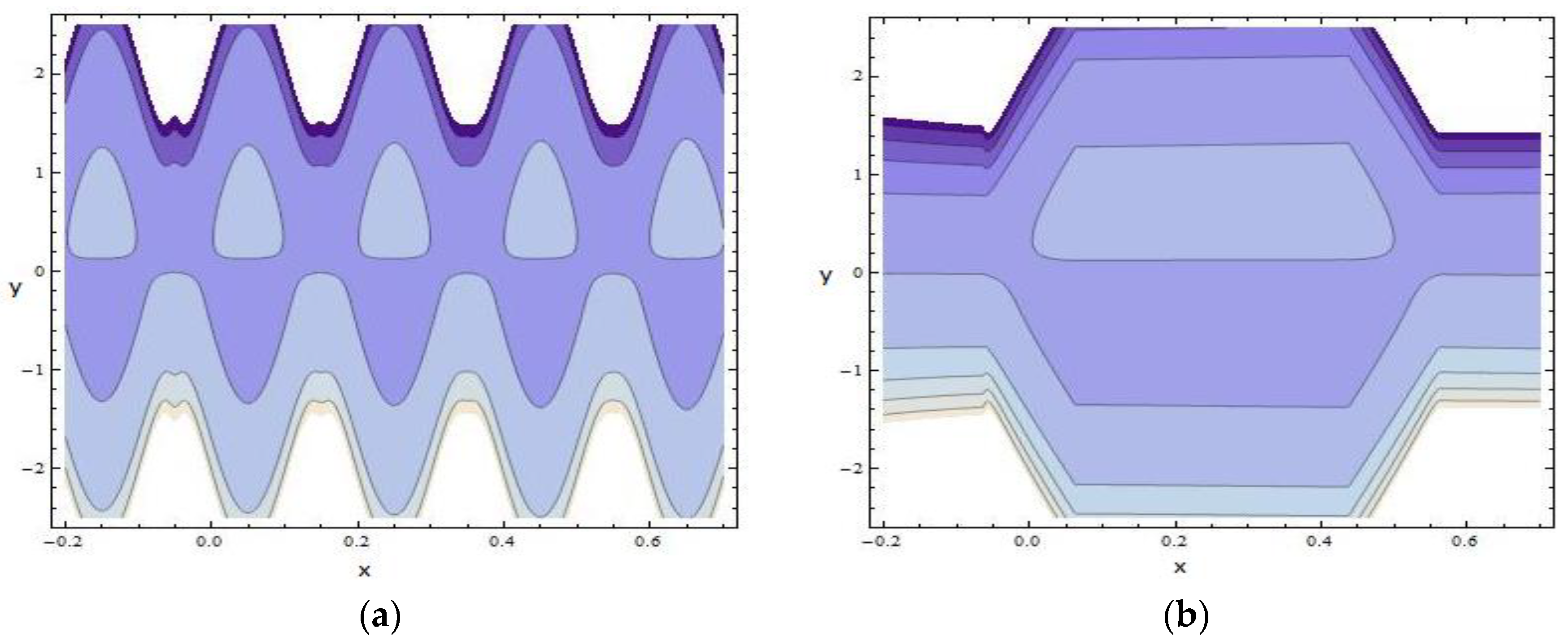
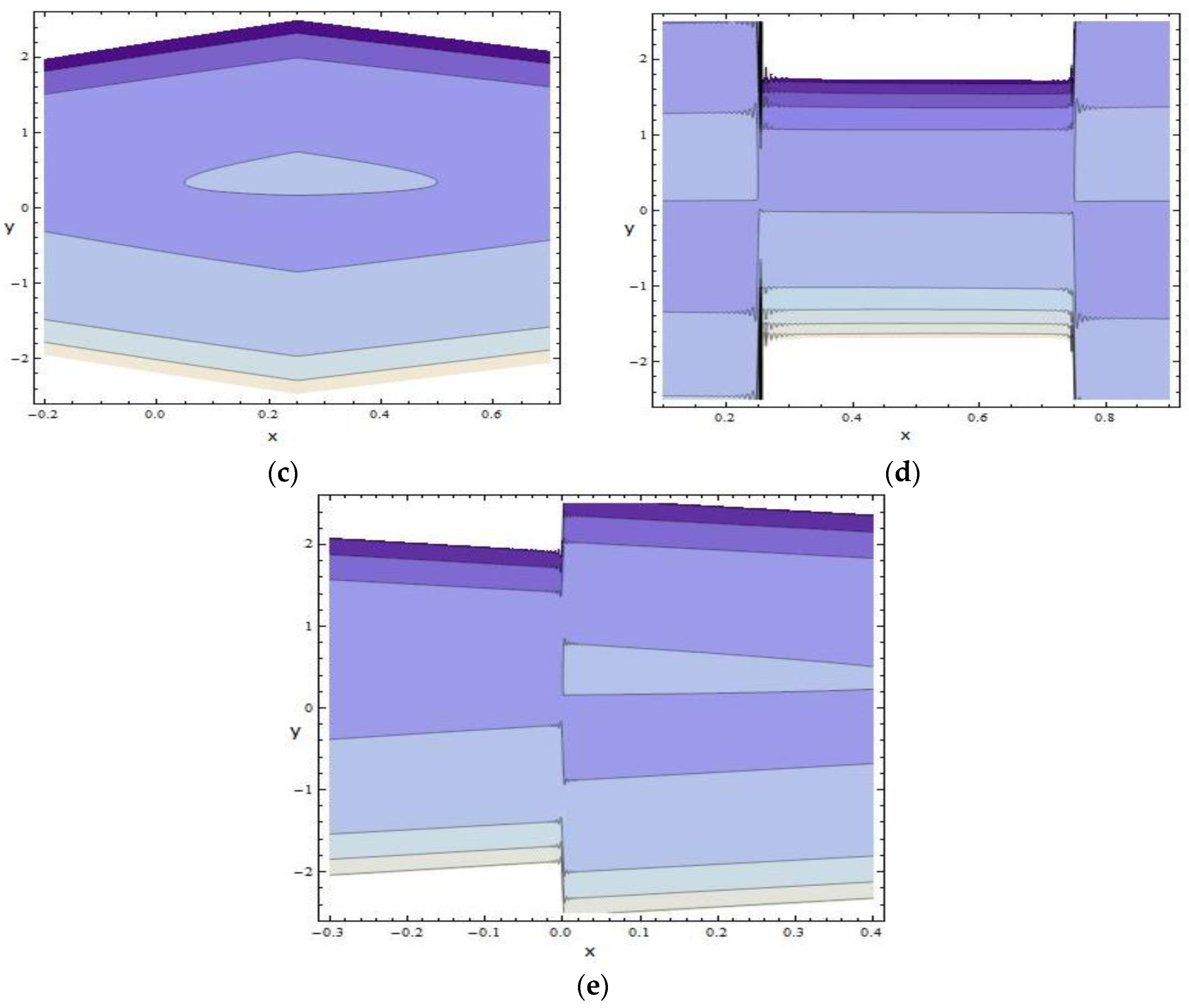
4. Different Wave Shapes

Non-dimensional expressions for six considered wave forms are given as [43]. Expressions for sinusoidal, multisinsoidal, triangular, square, trapezoidal and sawtooth waves are derived from the Fourier series.
Sinusoidal wave:
h 1 ( x ) = 1 + k x + a sin 2 π x , h 2 ( x ) = d k x b sin ( 2 π x + φ )
Multisinsoidal wave:
h 1 ( x ) = 1 + k x + a sin 2 n π x , h 2 ( x ) = d k x b sin ( 2 n π x + φ )
Triangular wave:
h 1 ( x ) = 1 + k x + a [ 8 π 3 m = 1 ( 1 ) m + 1 ( 2 m 1 ) 2 sin ( 2 π ( 2 m 1 ) x ) ] h 2 ( x ) = d k x b [ 8 π 3 m = 1 ( 1 ) m + 1 ( 2 m 1 ) 2 sin ( 2 π ( 2 m 1 ) x + φ ) ]
Trapezoidal wave:
h 1 ( x ) = 1 + k x + a [ 32 π 2 m = 1 sin π 8 ( 2 m 1 ) ( 2 m 1 ) 2 sin ( 2 π ( 2 m 1 ) x ) ] h 2 ( x ) = d k x b [ 32 π 2 m = 1 sin π 8 ( 2 m 1 ) ( 2 m 1 ) 2 sin ( 2 π ( 2 m 1 ) x + φ ) ]
Square wave:
h 1 ( x ) = 1 + k x + a [ 4 π m = 1 ( 1 ) m + 1 ( 2 m 1 ) cos ( 2 ( 2 m 1 ) π x ) ] h 2 ( x ) = d k x b [ 4 π m = 1 ( 1 ) m + 1 ( 2 m 1 ) cos ( 2 ( 2 m 1 ) π x + φ ) ]
Sawtooth wave:
h 1 ( x ) = 1 + k x + a [ 8 π 3 m = 1 sin ( 2 π m x ) m ] h 2 ( x ) = d k x b [ 8 π 3 m = 1 sin ( ( 2 π m x ) + φ ) m ]

5. Special Cases

If η 1 = η 2 = β = γ = k = 0 , results of Nadeem and Akram [24] can be recovered as a special case for present study. In addition to the vanishing of these values and in absence of heat and mass transfer, the following results can be obtained as further special cases:
  • Kothandapani and Srinivas [26], when Θ = α = 0 ,
  • Srinivas and Pushparaj [30], for Θ = λ 1 = 0 and
  • Mishra and Rao [42], at Θ = M = α = λ 1 = 0 .

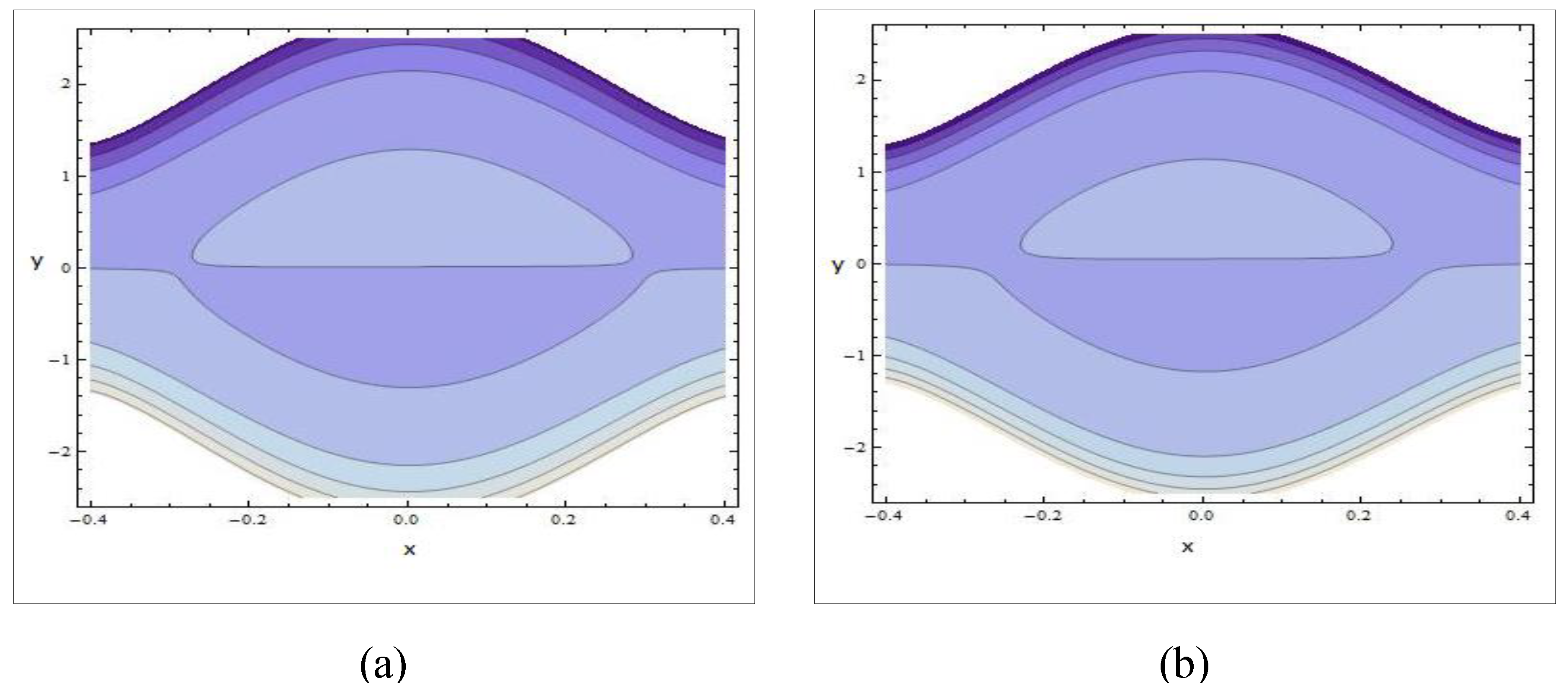
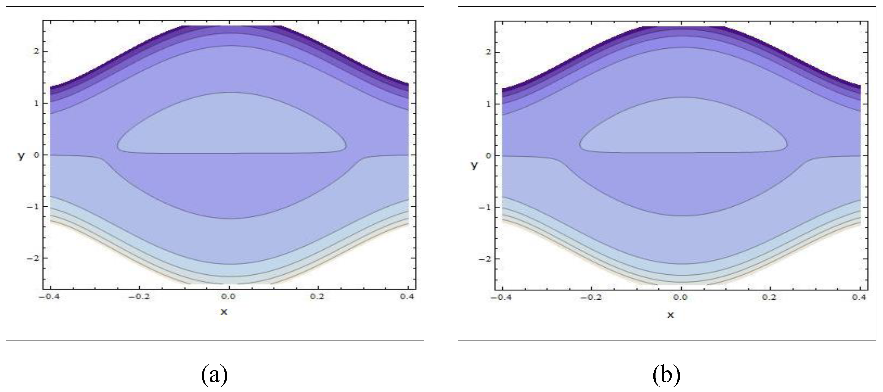
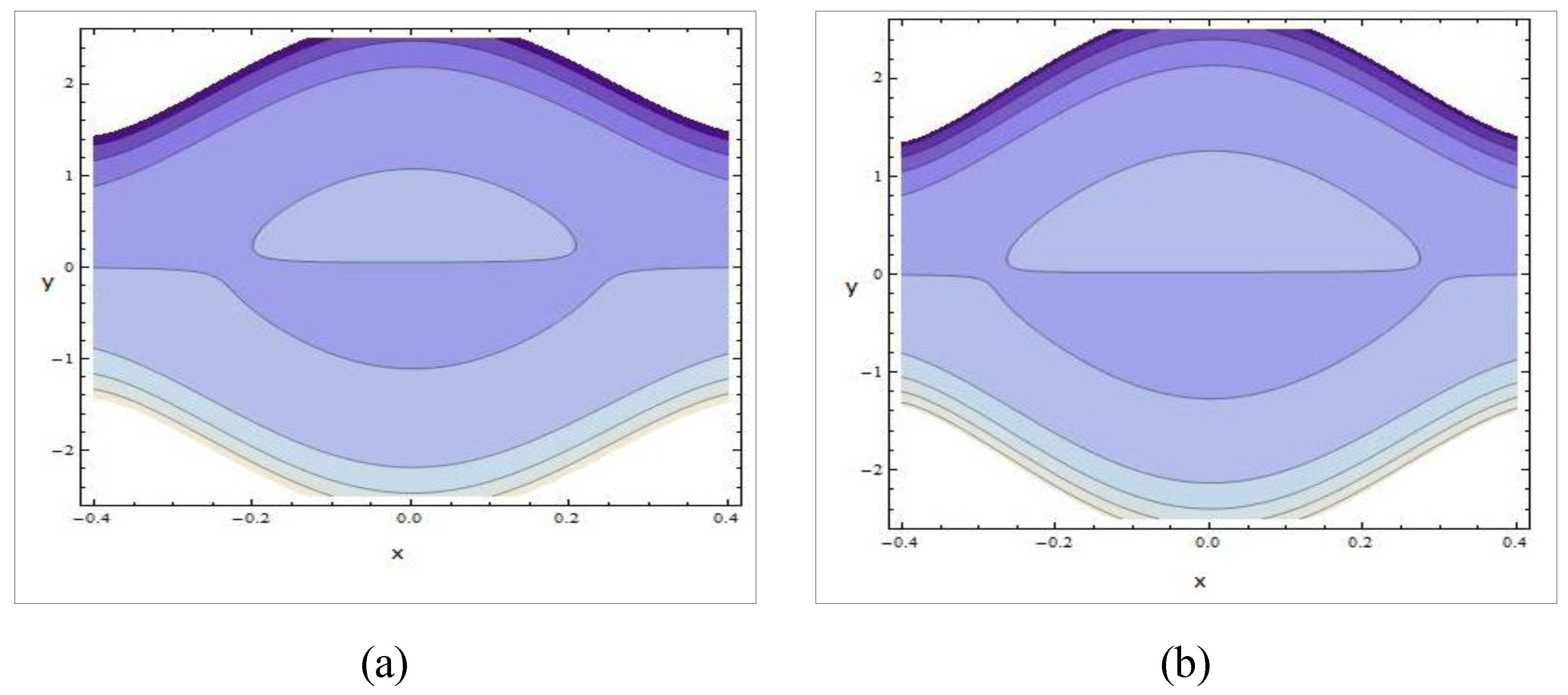
6. Results and Discussion

In the proceeding section, numerical results of current problems are conferred through graphs. Mathematica software is utilized to analyze expressions for pressure gradient and pressure rise numerically.
Figure 1, Figure 2, Figure 3 and Figure 4 are displayed to observe behaviour of pressure rise for diverse values of Jeffrey parameter λ 1 , non-uniform parameter k , Reynolds number Re and inclination angle Θ . It is noted from Figure 1; Figure 2 that behaviour of pressure rise decreases in retrograde pumping ( Δ p > 0 , Q < 0 ) , peristaltic pumping ( Δ p > 0 , Q > 0 ) and free pumping ( Δ p = 0 ) regions with an increase in λ 1 and k , whereas the behaviour of pressure rise is quite opposite in the co-pumping region ( Δ p < 0 , Q > 0 ) . In this region, with an increase in λ 1 and k , pressure rise increases. Figure 3 presents the behaviour of pressure rise for diverse values of Re . From this figure, we depicted that pressure rise increases in all pumping regions with an increase in values of Re . It is shown from Figure 4 that in the retrograde pumping ( Δ p > 0 , Q < 0 ) region, pressure rise increases with an increase in Θ , whereas in the co-pumping region ( Δ p < 0 , Q > 0 ) , behaviour of pressure rise decreases with an increase in Θ .
Figure 5, Figure 6, Figure 7 and Figure 8 are plotted in order to notice the behaviour of pressure gradient for various values of α , Jeffrey parameter λ 1 , Hartmann number M and non-dimensional slip parameters η 1 and η 2 . It is illustrated that for x [ 0 , 0.2 ] and x [ 0.8 , 1 ] , the pressure gradient is small so that flow can easily pass without the compulsion of a large pressure gradient, whereas in region x [ 0.2 , 0.8 ] , the pressure gradient increases with an increase in α , and it decreases with an increase in λ 1 , M , η 1 and η 2 , so more pressure gradient is necessary to maintain the flux to pass. Figure 9 shows the behaviour of the pressure gradient for diverse wave forms. It has been observed from Figure 9 that pressure gradient is maximum for square waves.
The behaviour of temperature profiles for diverse values of E c , λ 1 and Pr are shown in Figure 10, Figure 11 and Figure 12. It has been observed from Figure 10 that the temperature profile increases with an increase in E c . This phenomena is physically valid as E c shows a direct connection with temperature profile. Figure 11 depicts variation of the temperature profile for diverse values of λ 1 . It has been observed from Figure 11 that the temperature profile decreases with an increase in λ 1 . It has been observed from Figure 12 that the temperature profile increases with an increase in values of Pr . This happens due to the direct relation of Pr with the temperature profile.
Figure 13, Figure 14 and Figure 15 demonstrate theconcentration profile for diverse values of E c , λ 1 , S r and S c . It has been observed from Figure 13, Figure 14 that concentration profiles show opposite behaviour in comparison with the temperature profile. This observable fact physically holds as the temperature profile shows its inverse relationship with the concentration profile. It has been observed from Figure 13 that the concentration profile decreases with an increase in values of E c . It has been depicted from Figure 14 that with an increase in λ 1 that the concentration profile increases. Figure 15 shows the concentration profile for diverse values of S r and S c . It has been shown in Figure 15 that the concentration profile decreases with an increase in S r and S c .
In addition, an interesting observable fact in peristaltic flow is trapping. This is basically a pattern of an internally circulating bolus of fluid via closed stream lines. The trapping phenomena is discussed for different values of λ 1 , M , η 1 and η 2 . It has been observed from Figure 16, Figure 17 and Figure 18 that the size of the trapping bolus decreases with an increase in values of λ 1 , M , η 1 and η 2 . Figure 19 shows the behaviour of stream lines for diverse wave forms. It has been observed that in all considered wave forms that the trapped bolus increases in size and its size is smaller in the case of the triangular wave when compared with the other three wave forms. Figure 20 shows comparison of the present work with existing literature. It is observed in this figure that the exact solution of the present work and existing literature satisfies the boundary conditions. Moreover, the magnitude value of the velocity profile is maximum in the case of the present work and Nadeem and Akram [24]. In order to show the comparison of the present work with existing literature in tabular form, Table 1 is constructed.

7. Conclusions

In this research, we have investigated the effect of velocity second slip on non-Newtonian fluids by heat and mass transfer in the presence of an inclined magnetic field over an inclined tapered asymmetric channel. Governing equations of motion, energy and concentration were simplified via assumptions of long wavelength approximation. Then, exact solutions of reduced equations were calculated. Graphical results were plotted and reported for various involved physical parameters of concern. The main results can be typified as:
  • The results presented in [24,26,30,42] were considered as special cases of the present work.
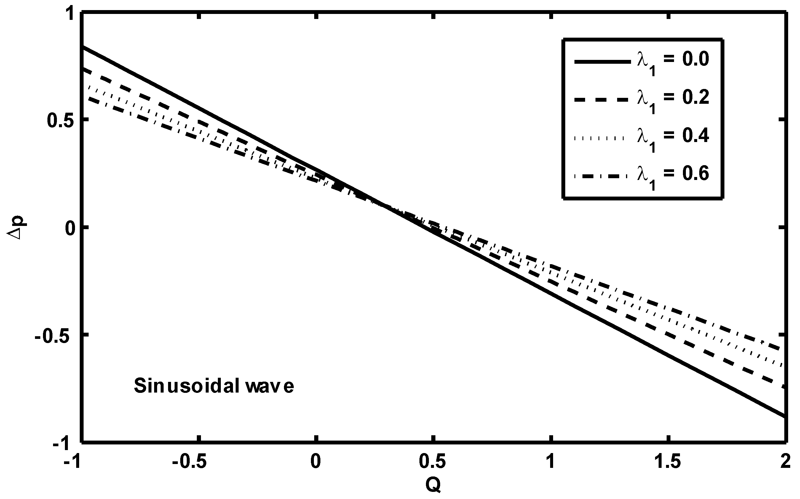
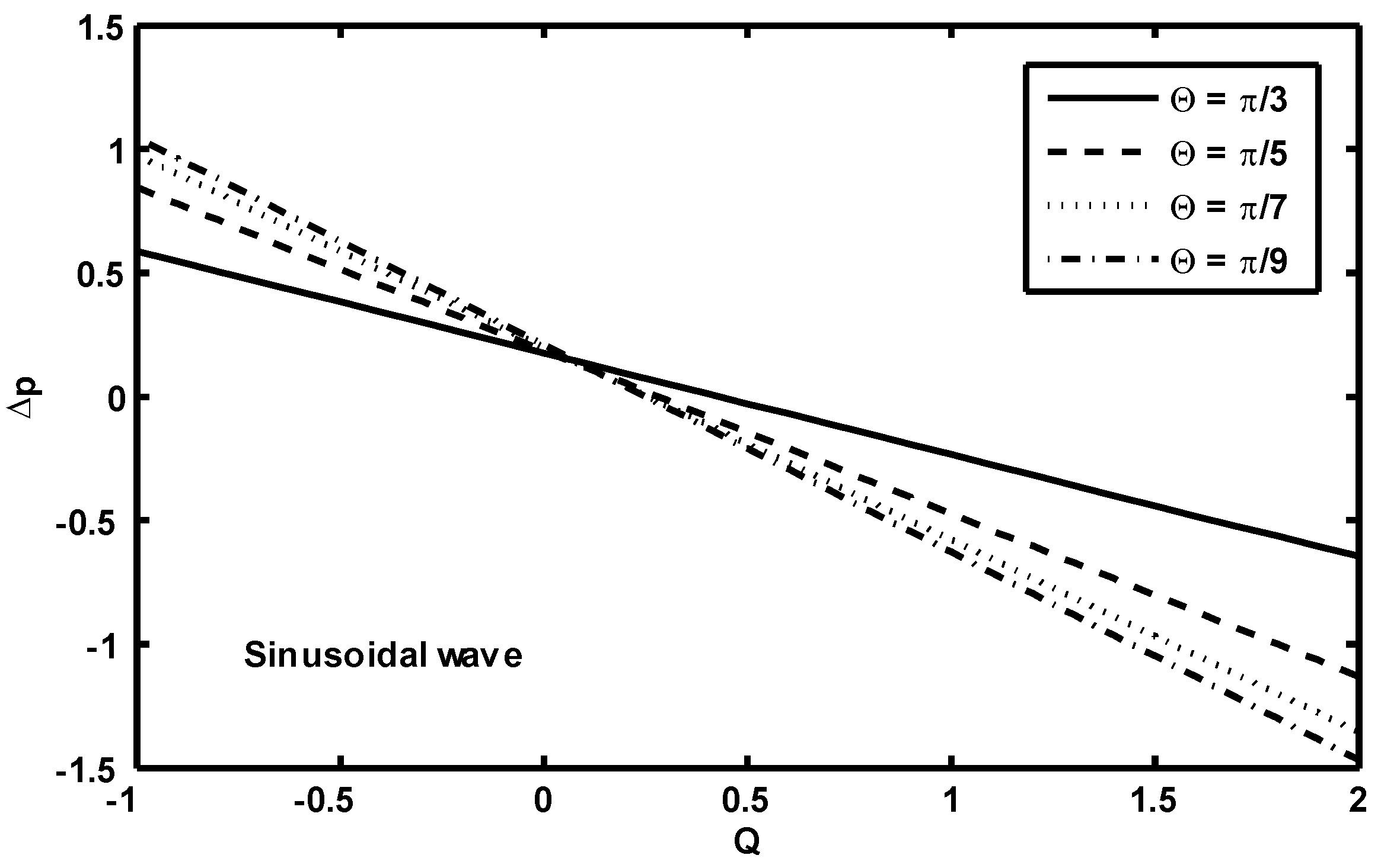
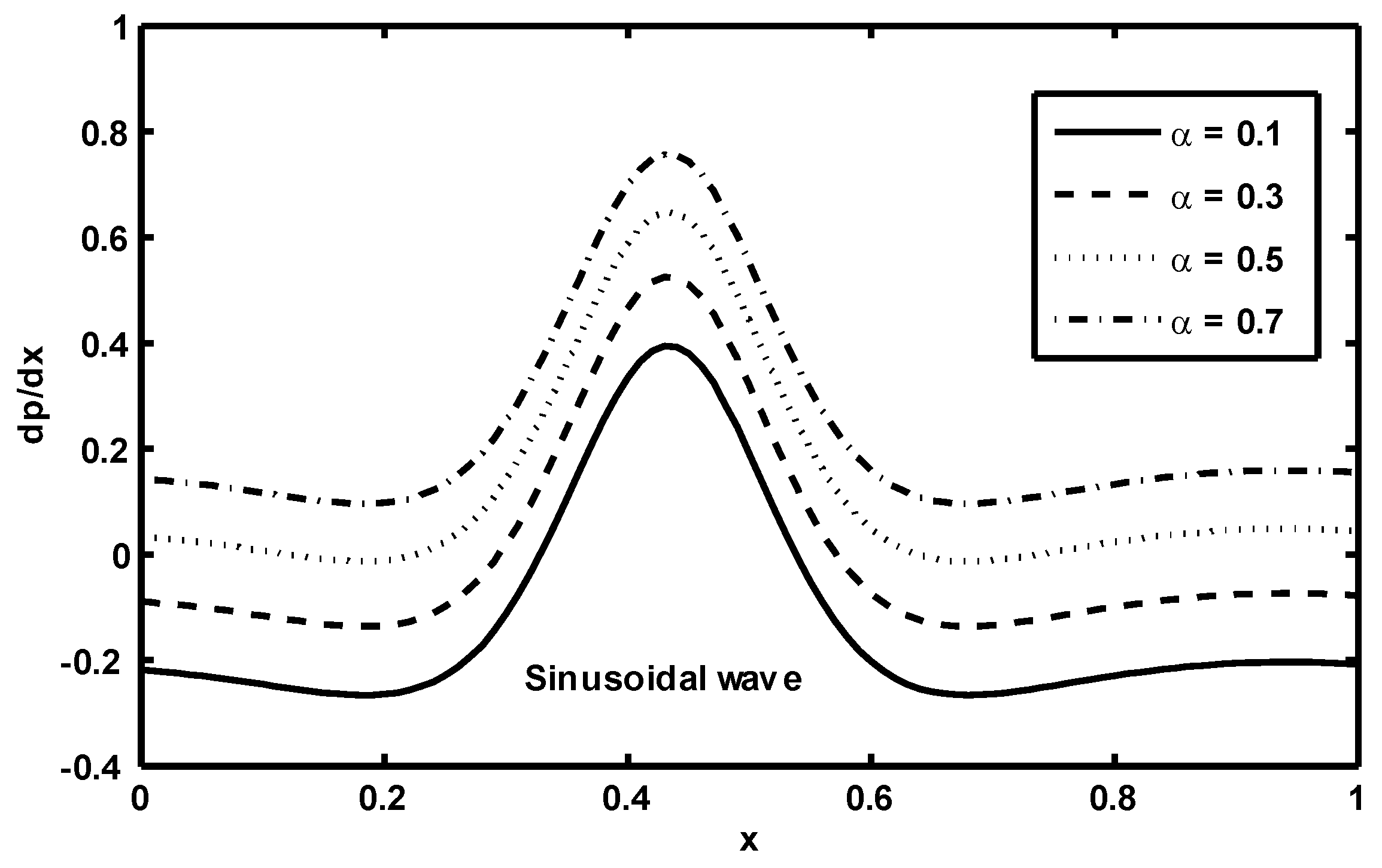
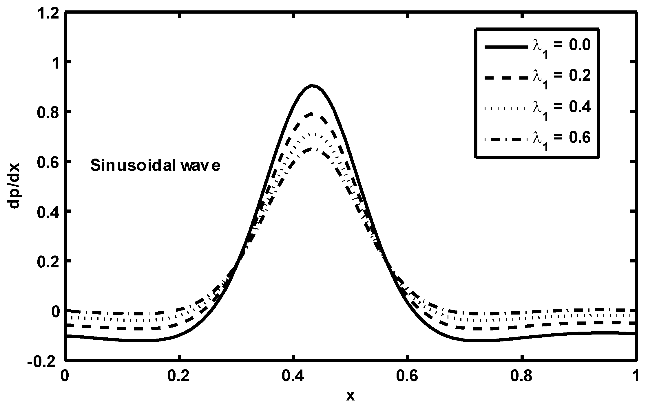
  • The pressure rise decreases in retrograde, peristaltic and free pumping regions and increases in co-pumping regions, with an increase in relaxation to retardation times λ 1 and non-uniform parameter k .
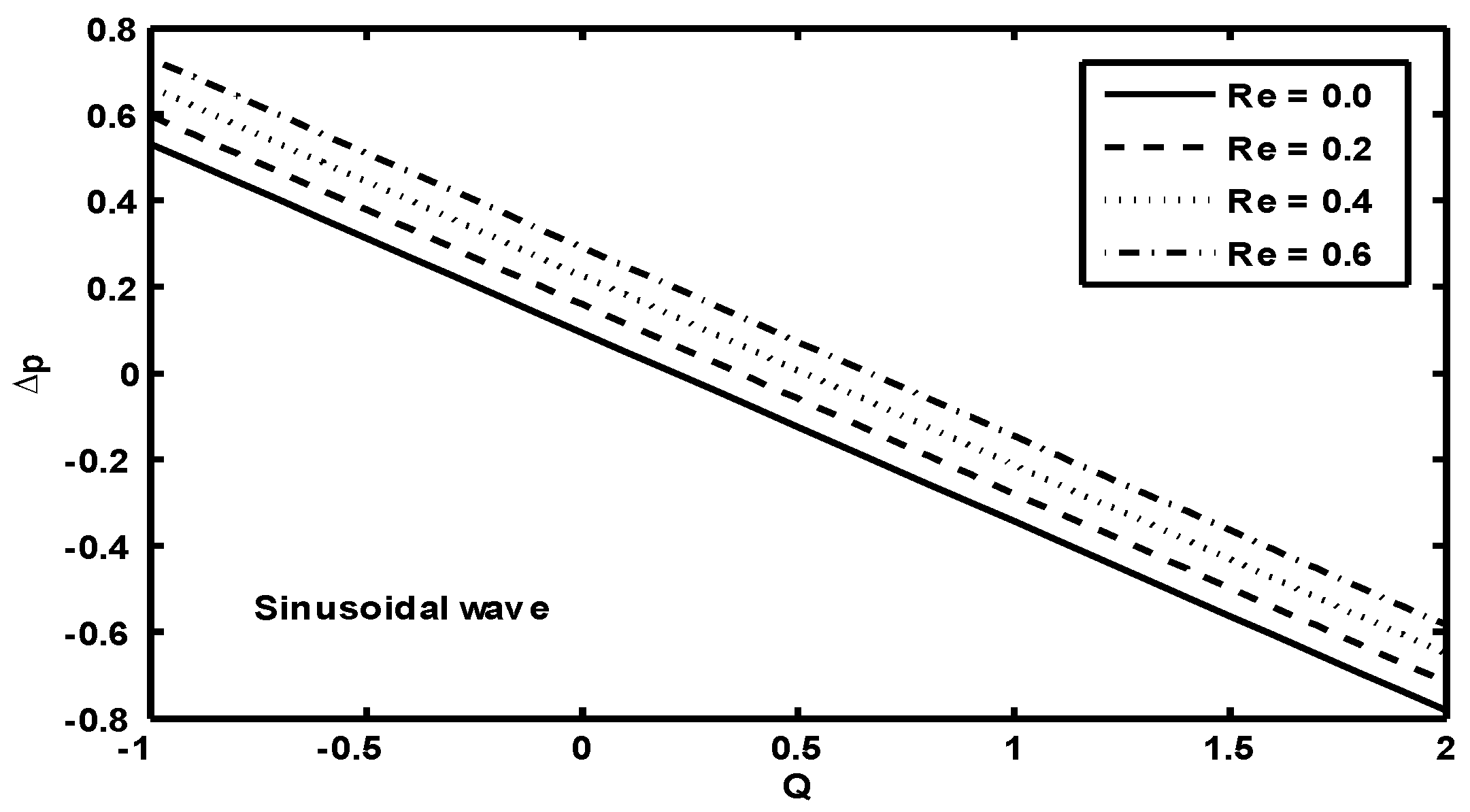
  • The pressure rise increases in all pumping regions with an increase in Reynolds number Re .
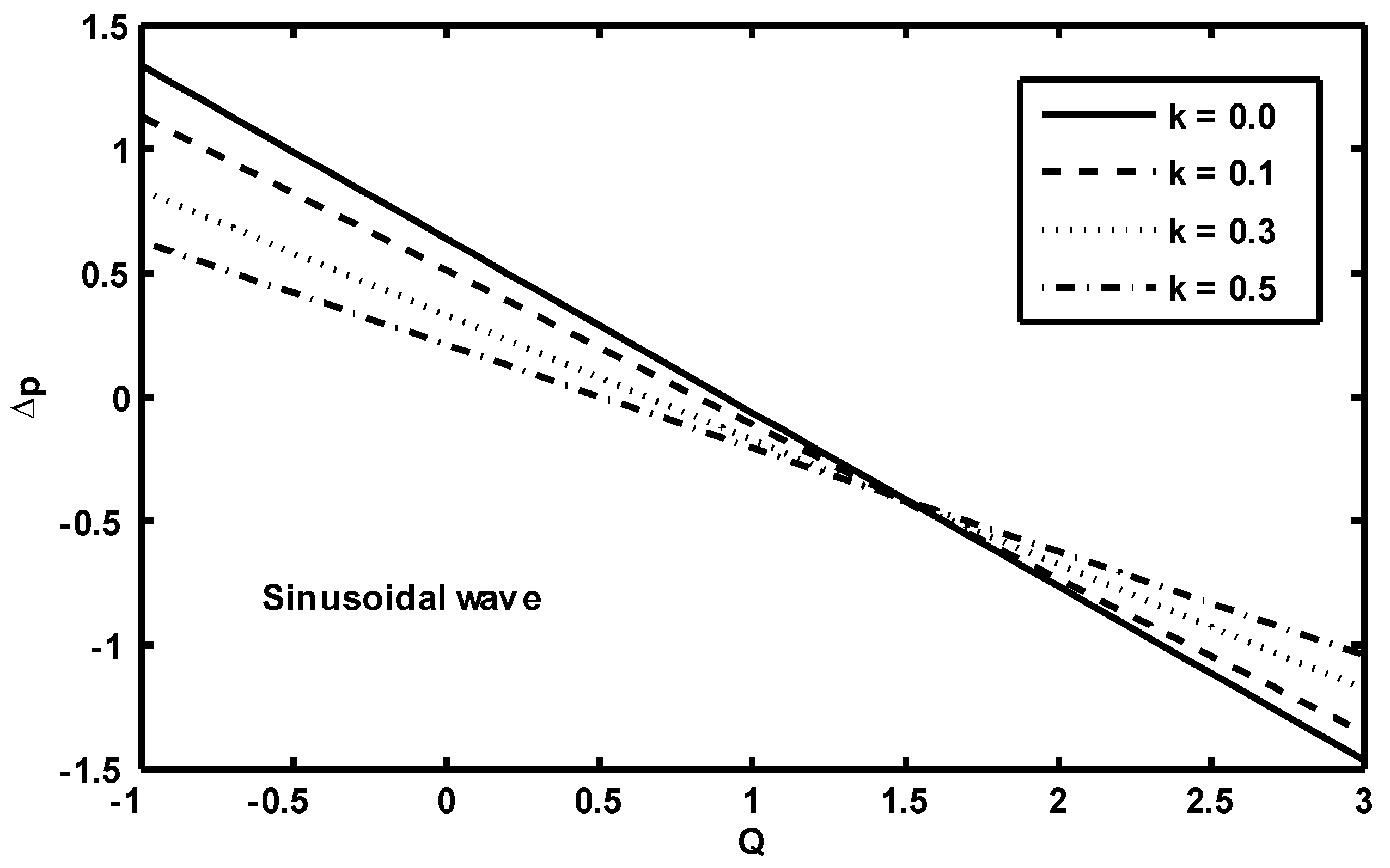
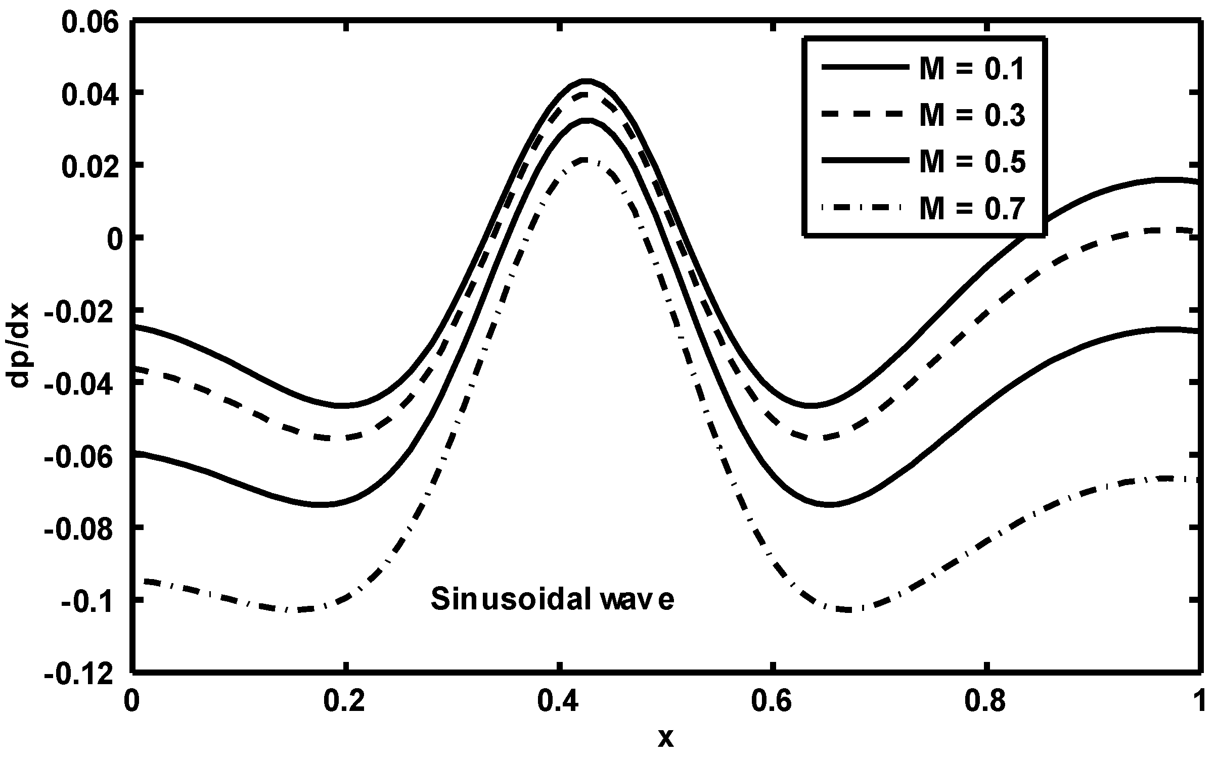
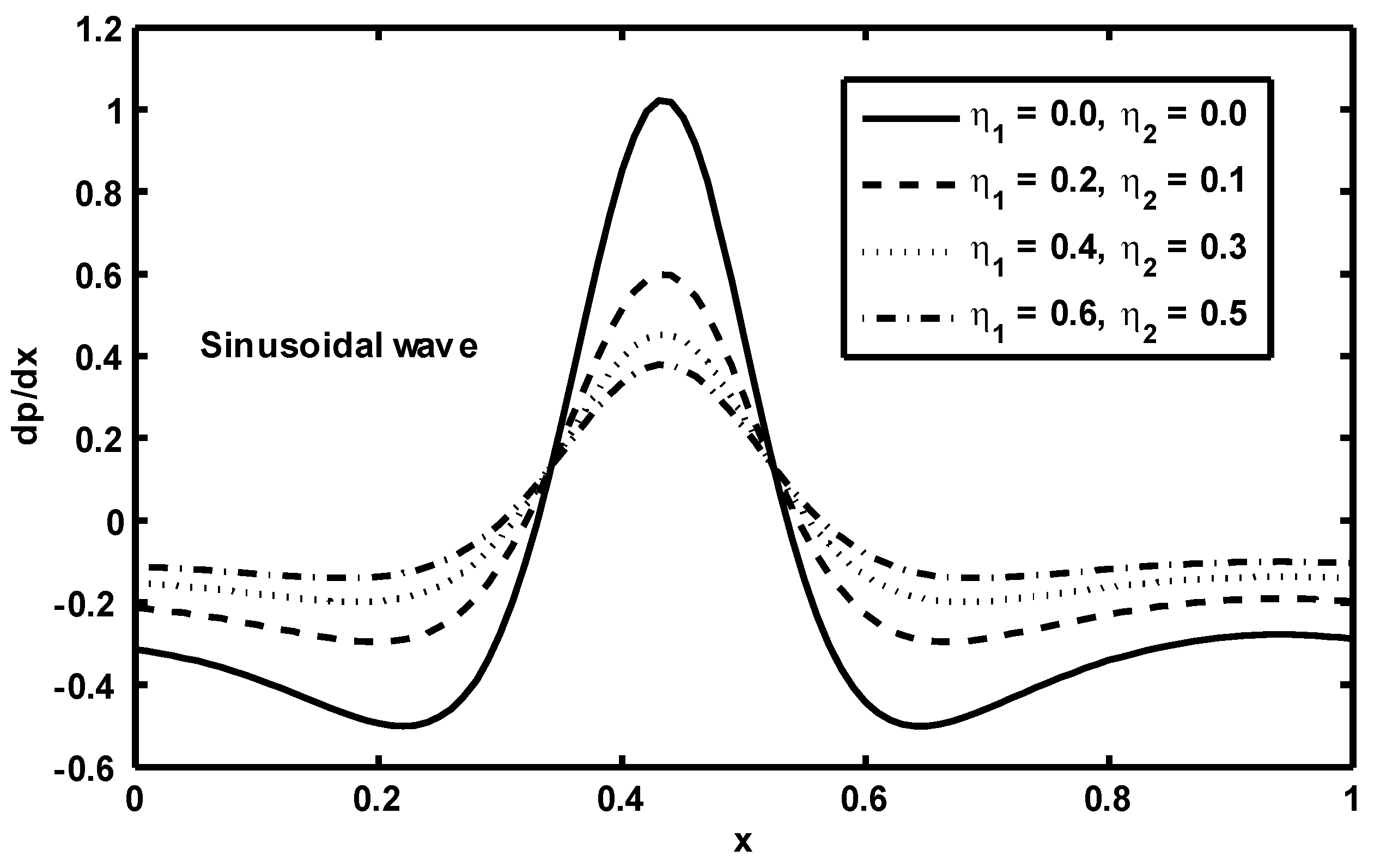
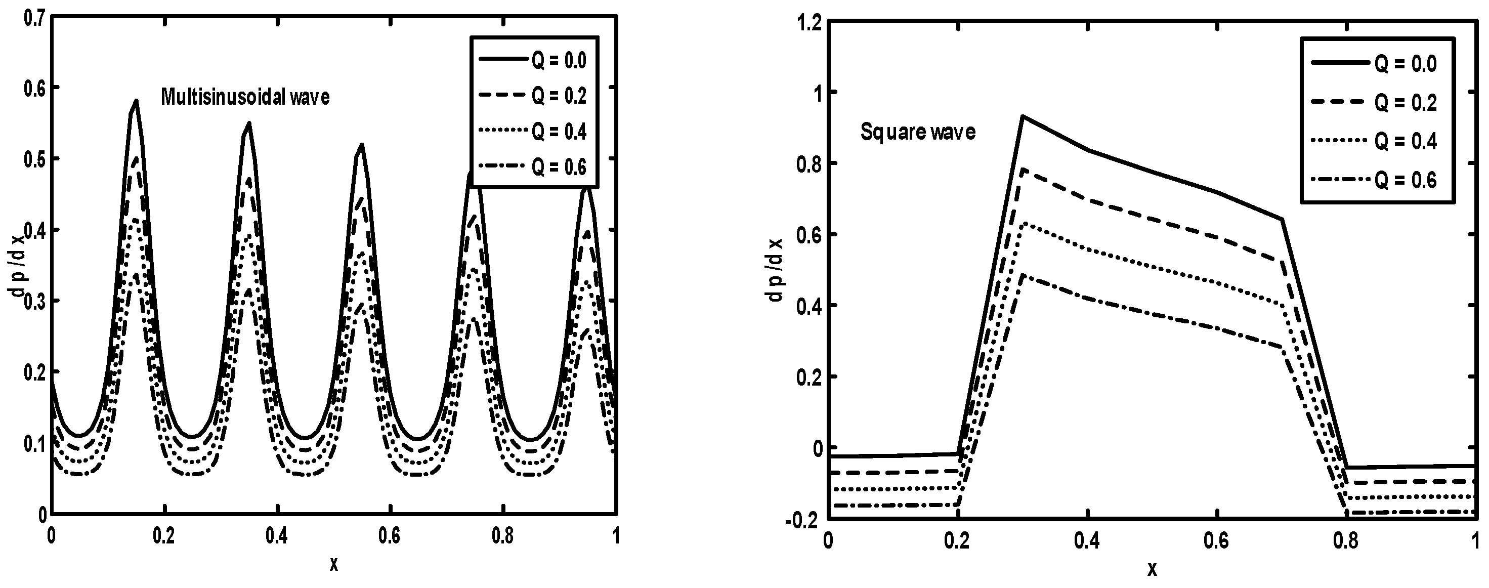
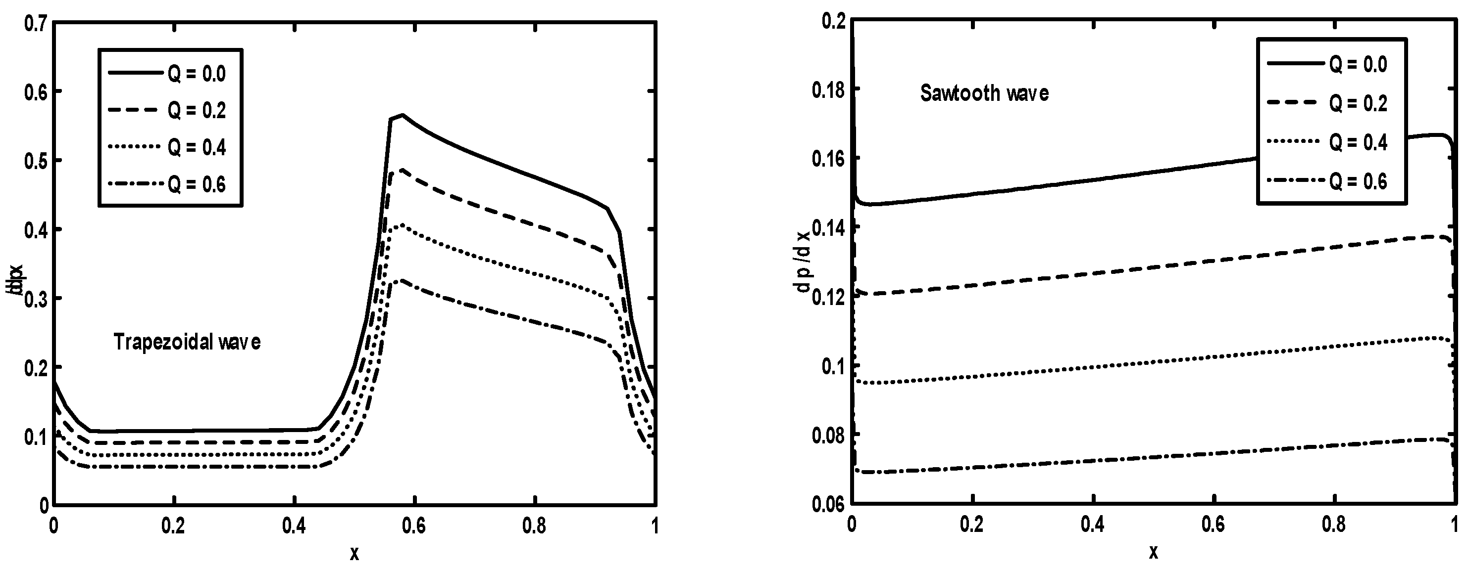
  • The pressure gradient increases with an increase in α and decreases with an increase in λ 1 , Hartmann number M , slip parameter η 1 and η 2 .
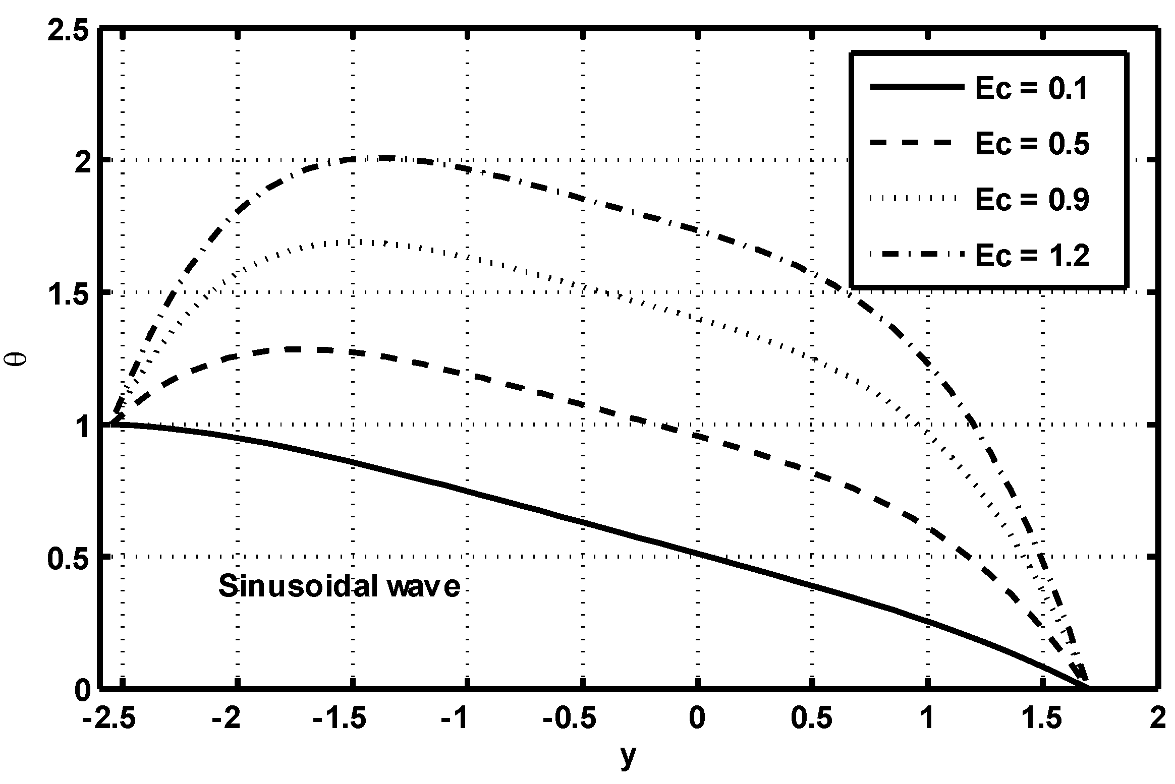
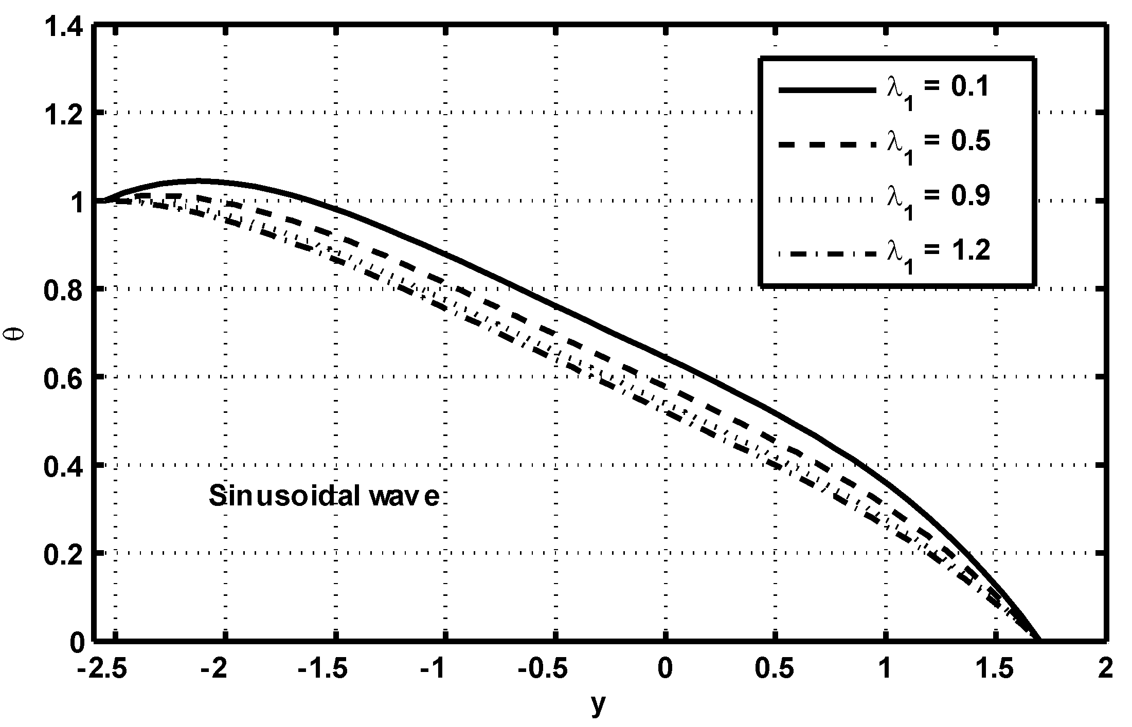
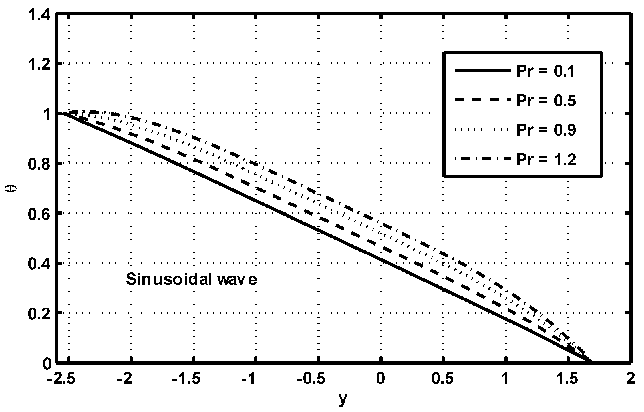
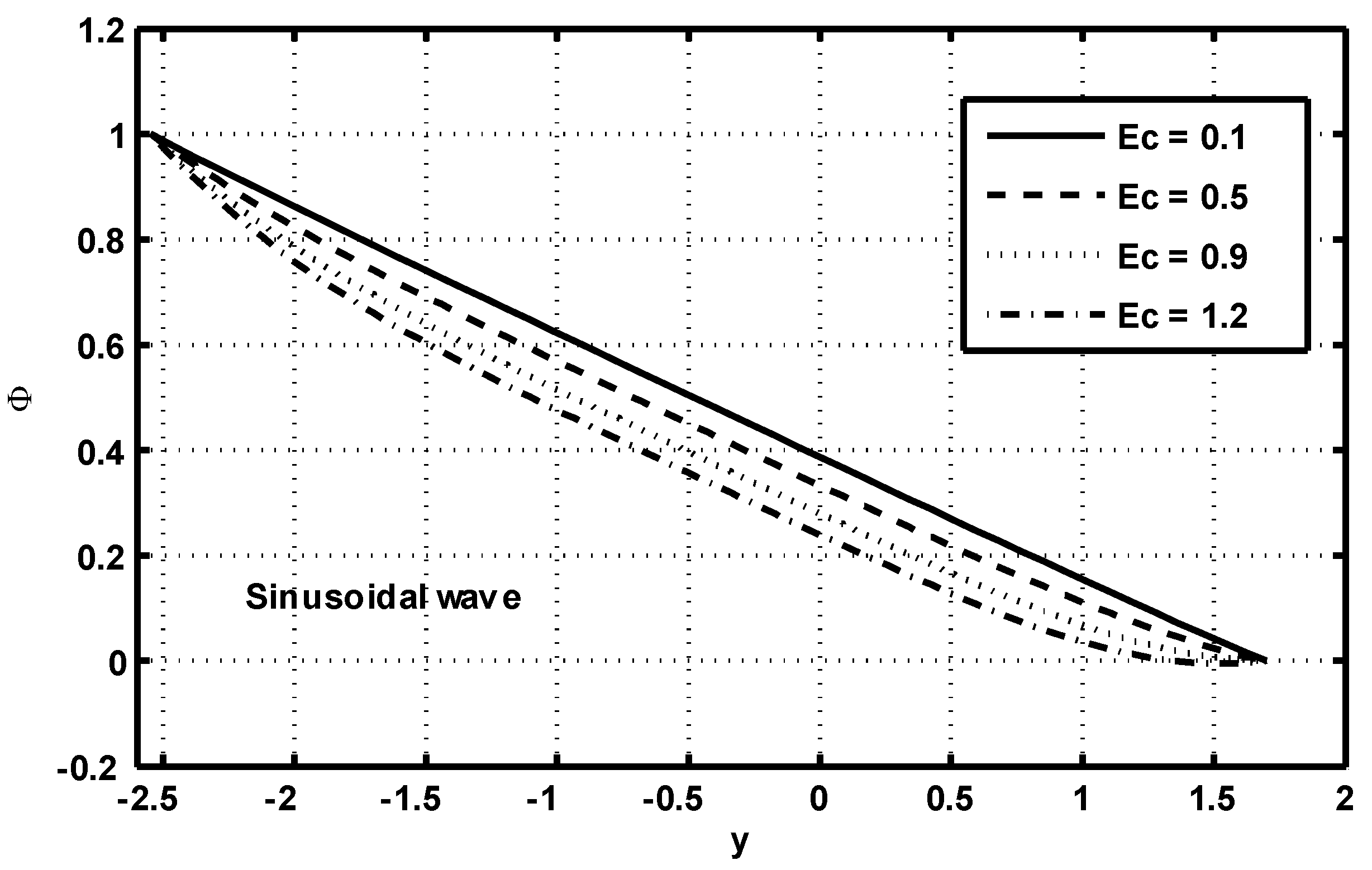
  • The temperature profile increases with an increase in values of Eckret number E c and decreases with an increase in relaxation to retardation times λ 1 .
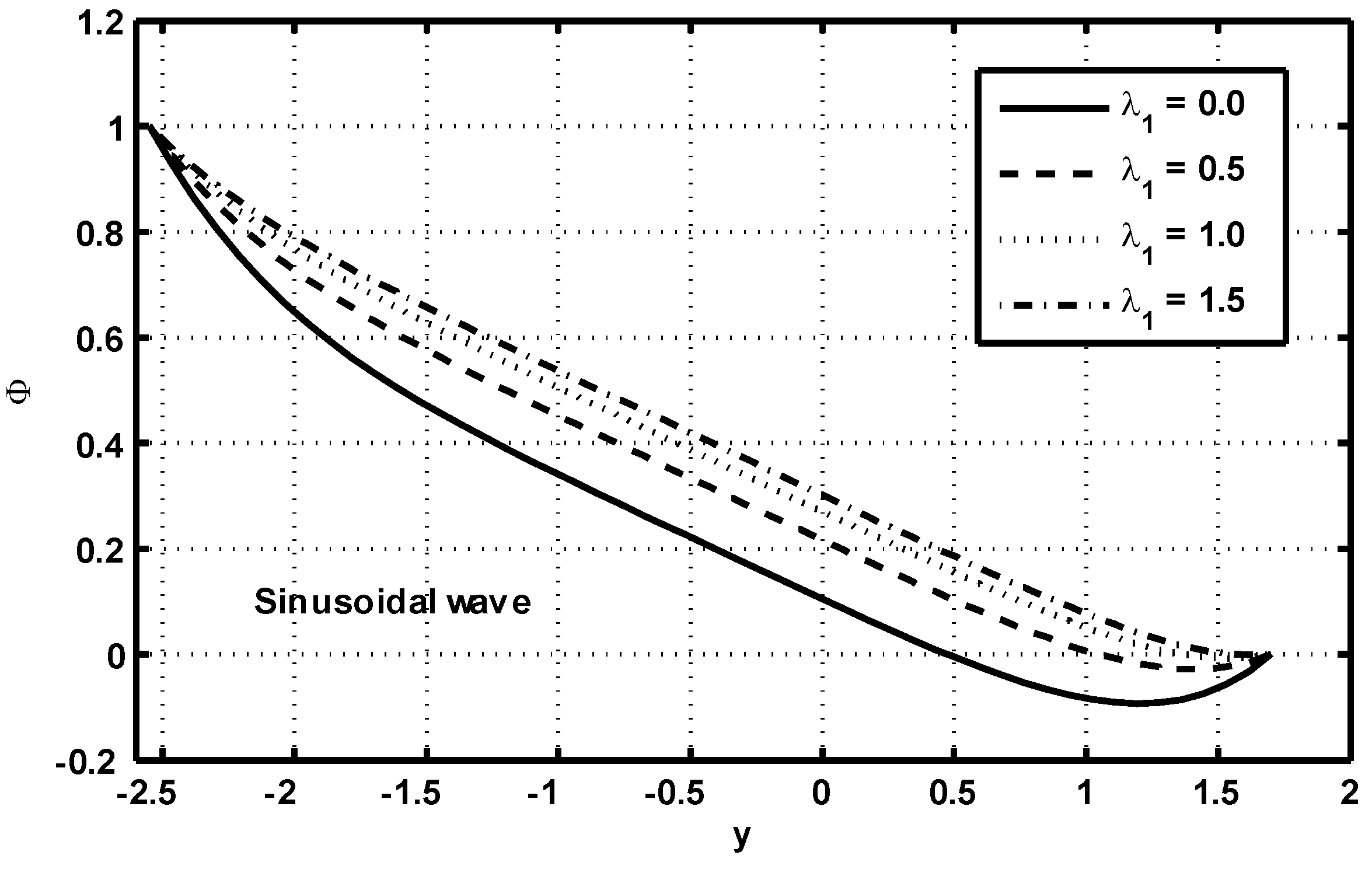
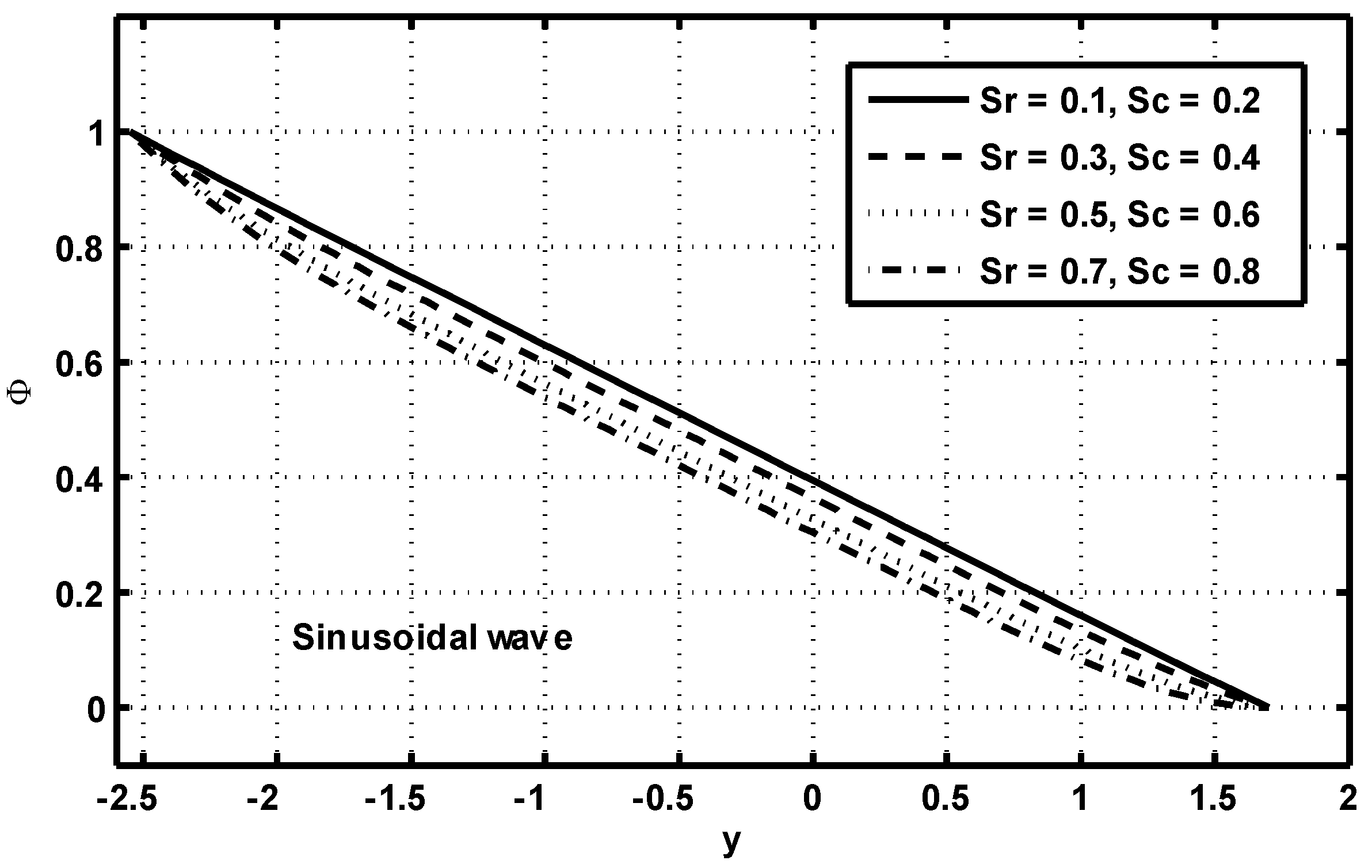
  • The concentration profile decreases with an increase in Soret number S r and Schmidt number S c .
  • The size of the trapping bolus decreases with an increase in values of relaxation to retardation times λ 1 , Hartmann number M , slip parameter η 1 and η 2 .

Author Contributions

Conceptualization, S.A. and E.H.A.; methodology, S.A.; software, N.S.; validation, S.A., N.S. and F.A.; formal analysis, A.H.; investigation, N.S.; resources, S.A.; data curation, E.H.A.; writing—original draft preparation, S.A.; writing—review and editing, E.H.A.; visualization, F.A.; supervision, S.A.; project administration, A.H.; funding acquisition, N.S. All authors have read and agreed to the published version of the manuscript.

Funding

This research received no external funding.

Acknowledgments

The authors would like to acknowledge the support provided by the Deanship of Scientific Research (DSR) at the Prince Mohammad Bin Fahd University (PMU) for funding this work.

Conflicts of Interest

The authors declare no conflict of interest.

Nomenclature

U , V Velocities in X and Y directions in fixed frame F r Froude Number
P Pressure S r Soret number
a 1 and b 1 amplitudes of waves d 1 + d 2 width of channel
k ( k < < 1 )non-uniform parameter λ wavelength
λ 1 ratio of relaxation to retardation times λ 2 retardation time
b amplitude of the wave S c Schmidt number
Re Reynolds number E c Eckret number
δ dimensionless wave number Pr Prandtl number
M Hartmann number μ viscosity
Q volume flow rate Ψ Stream function
ν kinematic viscosity Φ concentration of fluid in dimensionless form
θ temperature of fluid in dimensionless formCConcentration of fluid
σ electrical conductivity K T thermal diffusion ratio
K 1 thermal conductivity C p specific heat
T m mean temperature D m coefficient of mass diffusivity

Appendix A

L = 4 ( η 1 ( h 1 h 2 ) m 2 1 ) cosh ( ( h 1 h 2 ) m ) 2 m ( 2 η 1 + h 1 ( η 2 2 m 4 η 1 2 m 2 1 ) + h 2 ( η 2 2 m 4 + η 1 2 m 2 + 1 ) ) sinh ( ( h 1 h 2 ) m ) + 4 L 0 = 8 ( λ 1 + 1 ) ( 2 ( η 1 ( h 2 h 1 ) m 2 + 1 ) cosh ( ( h 1 h 2 ) m ) 2 + m ( 2 η 1 + h 1 ( η 2 2 m 4 η 1 2 m 2 1 ) + h 2 ( η 2 2 m 4 + η 1 2 m 2 + 1 ) ) sinh ( ( h 1 h 2 ) m ) ) 2 L 1 = 2 m 2 ( γ + h 1 ) h 2 2 + ( 2 h 1 ( 4 γ + h 1 ) m 2 + 2 γ ( 2 m γ + sinh ( 2 m h 1 ) ) m + cosh ( 2 m h 1 ) ) h 2 γ ( cosh ( 2 m h 1 ) + cosh ( 2 m h 2 ) + 2 m γ ( sinh ( 2 m h 1 ) sinh ( 2 m h 2 ) ) ) h 1 ( 2 γ ( 2 γ + h 1 ) m 2 2 γ sinh ( 2 m h 2 ) m + cosh ( 2 m h 2 ) )
L 2 = 2 m 2 ( γ + h 1 ) h 2 2 + ( 2 h 1 ( 4 γ + h 1 ) m 2 + 2 γ ( sinh ( 2 m h 1 ) 2 m γ ) m + cosh ( 2 m h 1 ) ) h 2 γ ( cosh ( 2 m h 1 ) + cosh ( 2 m h 2 ) + 2 m γ ( sinh ( 2 m h 1 ) sinh ( 2 m h 2 ) ) ) + h 1 ( 2 γ ( 2 γ + h 1 ) m 2 + 2 γ sinh ( 2 m h 2 ) m cosh ( 2 m h 2 ) ) L 3 = m ( sinh ( m h 1 ) + sinh ( m h 2 ) ) η 1 + cosh ( m h 2 ) ( m 2 η 2 1 ) + cosh ( m h 1 ) ( η 2 m 2 + 1 ) L 4 = ( m ( cosh ( m h 1 ) + cosh ( m h 2 ) ) η 1 + sinh ( m h 2 ) ( m 2 η 2 1 ) + sinh ( m h 1 ) ( η 2 m 2 + 1 ) ) L 5 = ( 2 cosh ( m ( h 1 h 2 ) ) ( ( h 2 h 1 ) η 1 m 2 + 1 ) + m sinh ( m ( h 1 h 2 ) ) ( 2 η 1 + h 1 ( η 2 2 m 4 η 1 2 m 2 1 ) + h 2 ( η 2 2 m 4 + η 1 2 m 2 + 1 ) ) 2 ) 2
L 6 = m ( sinh ( m h 1 ) + sinh ( m h 2 ) ) η 1 + cosh ( m h 2 ) ( m 2 η 2 1 ) + cosh ( m h 1 ) ( η 2 m 2 + 1 ) L 7 = 2 m γ cosh ( 2 m h 2 ) ( γ + h 1 ) sinh ( 2 m h 2 ) ( γ + h 1 ) ( 2 m γ cosh ( 2 m h 1 ) + sinh ( 2 m h 1 ) ) ( γ h 2 ) L 8 = ( 2 ( η 1 ( h 2 h 1 ) m 2 + 1 ) cosh ( ( h 1 h 2 ) m ) + m ( 2 η 1 + h 1 ( η 2 2 m 4 η 1 2 m 2 1 ) + h 2 ( η 2 2 m 4 + η 1 2 m 2 + 1 ) ) sinh ( ( h 1 h 2 ) m ) 2 ) 2 L 9 = 2 m 2 ( β + h 1 ) h 2 2 ( 2 h 1 ( 4 β + h 1 ) m 2 + 2 β ( 2 m β + sinh ( 2 m h 1 ) ) m + cosh ( 2 m h 1 ) ) h 2 + β ( cosh ( 2 m h 1 ) + cosh ( 2 m h 2 ) + 2 m β ( sinh ( 2 m h 1 ) sinh ( 2 m h 2 ) ) ) + h 1 ( 2 β ( 2 β + h 1 ) m 2 2 β sinh ( 2 m h 2 ) m + cosh ( 2 m h 2 ) )
L 10 = 2 m 2 ( β + h 1 ) h 2 2 + ( 2 ( 2 β 2 + 4 h 1 β + h 1 2 ) m 2 2 β sinh ( 2 m h 1 ) m cosh ( 2 m h 1 ) ) h 2 + β ( cosh ( 2 m h 1 ) + cosh ( 2 m h 2 ) + 2 m β ( sinh ( 2 m h 1 ) sinh ( 2 m h 2 ) ) ) + h 1 ( 2 β ( 2 β + h 1 ) m 2 2 β sinh ( 2 m h 2 ) m + cosh ( 2 m h 2 ) ) L 11 = 2 m β cosh ( 2 m h 2 ) ( β + h 1 ) + sinh ( 2 m h 2 ) ( β + h 1 ) + ( 2 m β cosh ( 2 m h 1 ) + sinh ( 2 m h 1 )

References

  1. Hayat, T.; Saleem, N.; Ali, N. Effect of induced magnetic field on peristaltic transport of a Carreau fluid. Commun. Nonlinear Sci. Numer. Simul. 2010, 15, 2407–2423. [Google Scholar] [CrossRef]
  2. Ellahi, R.; Riaz, A.; Nadeem, S.; Ali, M. Peristaltic flow of Carreau fluid in a rectangular duct through a porous medium. Math. Probl. Eng. 2012, 2012, 329639. [Google Scholar] [CrossRef]
  3. Vajravelu, K.; Sreenadh, S.; Saravana, R. Combined influence of velocity slip, temperature and concentration jump conditions on MHD peristaltic transport of a Carreau fluid in a non-uniform channel. Appl. Math. Comput. 2013, 225, 656–676. [Google Scholar] [CrossRef]
  4. Vajravelu, K.; Sreenadh, S.; Babu, V.R. Peristaltic transport of a Hershel-Bulkley fluid in an inclined tube. Int. J. Non Linear Mech. 2005, 40, 83–90. [Google Scholar] [CrossRef]
  5. Sankar, D.S.; Hemalatha, K. Pulsatile flow of Herschel—Bulkley fluid through catheterized arteries—A mathematical model. Appl. Math. Model. 2007, 31, 1497–1517. [Google Scholar] [CrossRef]
  6. Tripathi, D. A mathematical model for the peristaltic flow of chyme movement in small intestine. Math. Biosci. 2011, 233, 90–97. [Google Scholar] [CrossRef]
  7. Khan, A.A.; Ellahi, R.; Gulzar, M.M.; Sheikholeslami, M. Effects of heat transfer on peristaltic motion of Oldroyd fluid in the presence of inclined magnetic field. J. Magn. Magn. Mater. 2014, 372, 97–106. [Google Scholar] [CrossRef]
  8. Nadeem, S.; Akram, S. Peristaltic flow of a Williamson fluid in ana symmetric channel. Commun. Nonlinear Sci. Numer. Simul. 2010, 15, 1705–1716. [Google Scholar] [CrossRef]
  9. Hayat, T.; Wang, Y.; Siddiqui, A.M.; Hutter, K. Peristaltic motion of a Johnson—Segalman fluid in a plannar channel. Math. Probl. Eng. 2003, 1, 1–23. [Google Scholar] [CrossRef]
  10. Hayat, T.; Javed, M.; Asghar, S. MHD peristaltic motion of Johnson—Segalman fluid in a channel with compliant walls. Phys. Lett. 2008, 372, 5026–5036. [Google Scholar] [CrossRef]
  11. Akbar, N.S.; Nadeem, S.; Hayat, T. Simulation of thermal and velocity slip on the peristaltic flow of a Johnson—Segalman fluid in an inclined asymmetric channel. Int. J. Heat Mass Transf. 2012, 55, 5495–5502. [Google Scholar] [CrossRef]
  12. Akbar, N.S. Influence of magnetic field on peristaltic flow of a Casson fluid in an asymmetric channel: Application in crude oil refinement. J. Magn. Magn. Mater. 2015, 378, 463–468. [Google Scholar] [CrossRef]
  13. Ellahi, R.; Wang, X.; Hameed, M. Effects of heat transfer and nonlinear slip on the steady flow of Couette fluid by means of chebyshev spectral method. Z. Fur Nat. A 2014, 69, 1–8. [Google Scholar] [CrossRef]
  14. Ellahi, R.; Zeeshan, A.; Hussain, F.; Asadollahi, A. Peristaltic blood flow of couple stress fluid suspended with nanoparticles under the influence of chemical reaction and activation energy. Symmetry 2019, 11, 276. [Google Scholar] [CrossRef] [Green Version]
  15. Abbas, M.A.; Bai, Y.Q.; Bhatti, M.M.; Rashidi, M.M. Three dimensional peristaltic flow of hyperbolic tangent fluid in non-uniform channel having flexible walls. Alex. Eng. J. 2016, 55, 653–662. [Google Scholar] [CrossRef] [Green Version]
  16. Ellahi, R.; Hassan, M.; Zeeshan, A.; Khan, A.A. The shape effects of nanoparticles suspended in HFE-7100 over wedge with entropy generation and mixed convection. Appl. Nanosci. 2016, 6, 641–651. [Google Scholar] [CrossRef] [Green Version]
  17. Abbas, M.A.; Bai, Y.; Rashidi, M.M.; Bhatti, M.M. Analysis of entropy generation in the flow of peristaltic nanofluids in channels with compliant walls. Entropy 2016, 18, 90. [Google Scholar] [CrossRef]
  18. Ellahi, R.; Hussain, F.; Ishtiaq, F.; Hussain, A. Peristaltic transport of Jeffrey fluid in a rectangular duct through a porous medium under the effect of partial slip: An application to upgrade industrial sieves/filters. Pramana 2019, 93, 34. [Google Scholar] [CrossRef]
  19. Mekheimer, K.S.; Abdelmaboud, Y. Peristaltic flow of a couple stress fluid in an annulus: Application of an endoscope. Phys. A Stat. Mech. Appl. 2008, 2403, 387. [Google Scholar] [CrossRef]
  20. Ellahi, R.; Rahman, S.U.; Nadeem, S.; Vafai, K. A Mathematical Study of Non-Newtonian Micropolar Fluid in Arterial Blood Flow through Composite Stenosis. J. Appl. Math. Inf. Sci. 2014, 8, 1–7. [Google Scholar] [CrossRef]
  21. Abd-Alla, A.M.; Abo-Dahab, S.M.; El-Shahrany, H.D. Effects of rotation and initial stress on peristaltic transport of fourth grade fluid with heat transfer and induced magnetic field. J. Magn. Magn. Mater. 2014, 49, 268–280. [Google Scholar] [CrossRef]
  22. Akram, S.; Nadeem, S. Influence of induced magnetic field and heat transfer on the peristaltic motion of a Jeffrey fluid in an asymmetric channel: Closed form solutions. J. Magn. Magn. Mater. 2013, 328, 11–20. [Google Scholar] [CrossRef]
  23. Hussain, Q.; Asghar, S.; Hayat, T.; Alsaedi, A. Heat transfer analysis in peristaltic flow of MHD Jeffrey fluid with variable thermal conductivity. Appl. Math. Mech. Engl. Ed. 2015, 36, 499–516. [Google Scholar] [CrossRef]
  24. Nadeem, S.; Akram, S. Influence of inclined magnetic field on peristaltic flow of a Jeffrey fluid with heat and mass transfer in an inclined symmetric or asymmetric channel. Asia Pac. J. Chem. Eng. 2012, 7, 33–44. [Google Scholar] [CrossRef]
  25. Akram, S.; Aly, E.H.; Nadeem, S. Effects of metachronal wave on biomagnetic Jeffery fluid with inclined magnetic field. Rev. Téc. Ing. Univ. Zulia. 2015, 38, 18–28. [Google Scholar]
  26. Kothandapani, M.; Srinivas, S. Peristaltic transport of a Jeffrey fluid under the effect of magnetic field in an asymmetric channel. Int. J. Non Linear Mech. 2008, 43, 915. [Google Scholar] [CrossRef]
  27. Tripathi, D.; Ali, N.; Hayat, T.; Chaube, M.K.; Hendi, A.A. Peristaltic flow of MHD Jeffrey fluid through finite length cylindrical tube. Appl. Math. Mech. 2011, 32, 1231–1244. [Google Scholar] [CrossRef]
  28. Nadeem, S.; Riaz, A.; Ellahi, R.; Mushtaq, M. Series solutions of magnetohydrodynamic peristaltic flow of a Jeffrey fluid in eccentric cylinders. J. Appl. Math. Inf. Sci. 2013, 7, 1441–1449. [Google Scholar]
  29. Khan, A.A.; Ellahi, R.; Vafai, K. Peristaltic transport of a Jeffrey fluid with variable viscosity through a porous medium in an asymmetric channel. Adv. Math. Phys. 2012, 2012. [Google Scholar] [CrossRef]
  30. Srinivas, S.; Pushparaj, V. Non-linear peristaltic transport in an inclined asymmetric channel. Commun. Nonlinear Sci. Numer. Simul. 2008, 13, 1782–1795. [Google Scholar] [CrossRef]
  31. Navier, C.L.M.H. Sur les lois du mouvement des fluids. Mem. Acad. R. Sci. Inst. Fr. 1827, 6, 389–440. [Google Scholar]
  32. Saleem, N.; Hayat, T.; Alsaedi, A. Effects of induced magnetic field and slip condition on peristaltic transport with heat and mass transfer in a non-uniform channel. Int. J. Phys. Sci. 2012, 7, 191–204. [Google Scholar]
  33. Ebaid, A.; Aly, E.H. Exact analytical solution of the peristaltic nanofluids flow in an asymmetric channel with flexible walls and slip condition: Application to the cancer treatment. Comput. Math. Meth. Med. 2013, 8. [Google Scholar] [CrossRef] [PubMed] [Green Version]
  34. Aly, E.H.; Ebaid, A. Exact analytical solution for the peristaltic flow of nanofluids in an asymmetric channel with slip effect of the velocity, temperature and concentration. J. Mech. 2014, 30, 411–422. [Google Scholar] [CrossRef]
  35. Srinivas, S.; Gayathri, R.; Kothandapani, M. The influence of slip conditions, wall properties and heat transfer on MHD peristaltic transport. Comput. Phys. Commun. 2009, 180, 2115–2122. [Google Scholar] [CrossRef]
  36. Hayat, T.; Hina, S.; Hendi, A.A. Peristaltic motion of power-law fluid with heat and mass transfer. Chin. Phys. Lett. 2011, 28, 084707. [Google Scholar] [CrossRef]
  37. Hayat, T.; Hina, S. The influence of wall properties on the MHD peristaltic flow of a Maxwell fluid with heat and mass transfer. Nonlinear Anal. Real World Appl. 2010, 11, 3155–3169. [Google Scholar] [CrossRef]
  38. Hayat, T.; Hina, S. Effects of heat and mass transfer on peristaltic flow of Williamson fluid in a non-uniform channel with slip conditions. Int. J. Numer. Methods Fluids 2011, 67, 1590–1604. [Google Scholar] [CrossRef]
  39. Nadeem, S.; Akram, S. Heat transfer in a peristaltic flow of MHD fluid with partial slip. Commun. Nonlinear Sci. Numer. Simul. 2010, 15, 312–321. [Google Scholar] [CrossRef]
  40. Hayat, T.; Noreen, S.; Hendi, A.A. Peristaltic motion of Phan-Thien-Tanner fluid in the presence of slip condition. J. Biorheol. 2011, 25, 8–17. [Google Scholar] [CrossRef]
  41. Hayat, T.; Khan, M.; Ayub, M. The effect of the slip condition on flows of an Oldroyd 6-constant fluid. J. Comput. Appl. Math. 2007, 202, 402–413. [Google Scholar] [CrossRef] [Green Version]
  42. Mishra, M.; Rao, A.R. Peristaltic transport of a Newtonian fluid in an asymmetric channel. ZAMP 2003, 54, 532–550. [Google Scholar] [CrossRef]
  43. Akram, S.; Nadeem, S. Significance of nanofluid and partial slip on the peristaltic transport of a non-Newtonian fluid with different waveforms. IEEE Trans. Nanotechnol. 2014, 13, 375–385. [Google Scholar] [CrossRef]
  44. Hina, S.; Mustafa, M.; Hayat, T.; Alotaibi, N. On peristaltic motion of pesudoplastic fluid in a curved channel with heat/mass transfer and wall properties. Appl. Math. Comput. 2015, 263, 378–391. [Google Scholar]
  45. Roşca, A.V.; Pop, I. Flow and heat transfer over a vertical permeable stretching/shrinking sheet with a second order slip. Int. J. Heat Mass Transf. 2013, 60, 355–364. [Google Scholar] [CrossRef]
  46. Aly, E.H. Radiation and MHD boundary layer stagnation—point of nanofluid flow towards a stretching sheet embedded in a porous medium: Analysis of suction/injection and heat generation/absorption with effect of the slip model. Math. Probl. Eng. 2015, 2015. Available online: www.Hindawi.com/Journals/mpe/aip/563647 (accessed on 8 May 2015). [CrossRef]
  47. Aly, E.H. Effect of the velocity slip boundary condition on the flow and heat transfer of nanofluids over a stretching sheet. J. Comput. Theor. Nanosci. 2015, in press. [Google Scholar] [CrossRef]
  48. Aly, E.H.; Vajravelu, K. Exact and numerical solutions of MHD nano boundary-layer flows over stretching surfaces in porous medium. Appl. Math. Comput. 2014, 232, 191–204. [Google Scholar] [CrossRef]
  49. Aly, E.H.; Ebaid, A. Effect of the velocity second slip boundary condition on the peristaltic flow of nanofluids in an asymmetric channel: Exact solution. Abstr. Appl. Anal. 2014, 2014. [Google Scholar] [CrossRef]
  50. Kothandapani, M.; Prakash, J. Effects of thermal radiation parameter and magnetic field on the peristaltic motion of Williamson nanofluids in a tapered asymmetric channel. Int. J. Heat Mass Transf. 2015, 81, 234–245. [Google Scholar] [CrossRef]
  51. Kothandapani, M.; Prakash, J. Effect of radiation and magnetic field on peristaltic transport of nanofluids through a porous space in a tapered asymmetric channel. J. Magn. Magn. Mater. 2015, 378, 152–163. [Google Scholar] [CrossRef]
  52. Kothandapani, M.; Prakash, J.; Srinivas, S. Peristaltic transport of a MHD Carreau fluid in a tapered asymmetric channel with permeable walls. Int. J. Biomath. 2015, 8. [Google Scholar] [CrossRef]
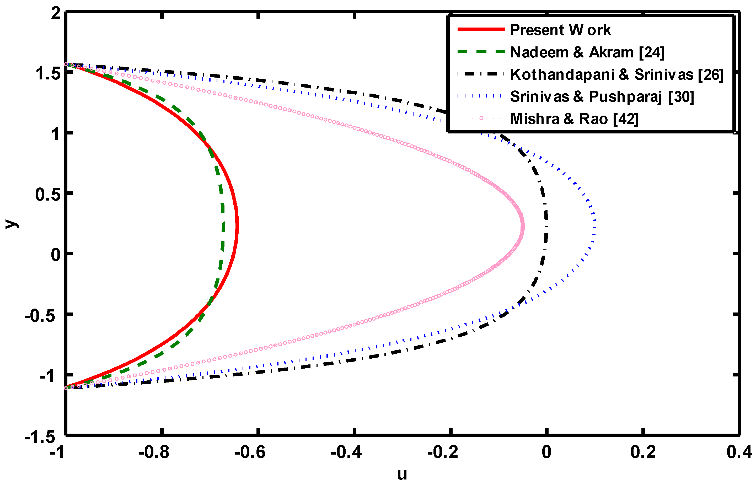
Figure 1. Variation of Δ p with Q for different values of λ 1 for fixed a = 0.7 , α = 0.2 , b = 0.7 , d = 1.5 , Θ = π 6 , M = 0.5 , Re = 0.4 , φ = π 4 , F r = 0.6 , η 1 = 0.3 , η 2 = 0.4 , k = 0.5 .
Coatings 10 00030 g001
Figure 2. Variation of Δ p with Q for different values of k for fixed a = 0.7 , α = 0.2 , b = 0.7 , d = 1.5 , Θ = π 6 , M = 0.5 , Re = 0.4 , φ = π 4 , F r = 0.6 , η 2 = 0.4 , η 1 = 0.5 , λ 1 = 0.1 .
Coatings 10 00030 g002
Figure 3. Variation of Δ p with Q for different values of Re for fixed a = 0.7 , α = 0.2 , b = 0.7 , d = 1.5 , Θ = π 6 , λ 1 = 0.4 , M = 0.5 , φ = π 4 , F r = 0.6 , η 1 = 0.3 , η 2 = 0.4 , k = 0.5 .
Coatings 10 00030 g003
Figure 4. Variation of Δ p with Q for different values of Θ for fixed a = 0.7 , α = 0.2 , b = 0.7 , d = 1.5 , λ 1 = 0.7 , M = 1 , R = 0.3 , φ = π 4 , F r = 0.6 , η 1 = 0.3 , η 2 = 0.4 , k = 0.5 .
Coatings 10 00030 g004
Figure 5. Variation of d p / d x with x for different values of α for fixed a = 0.7 , b = 0.7 , d = 1.5 , F r = 0.6 , Θ = π 3 , M = 0.5 , Re = 0.4 , φ = π 4 , η 1 = 0.4 η 2 = 0.5 , λ 1 = 0.3 , k = 0.1 , Q = 1 .
Coatings 10 00030 g005
Figure 6. Variation of d p / d x with x for different values of λ 1 for fixed a = 0.7 , α = 0.3 , b = 0.7 , d = 1.5 , Θ = π 3 , Re = 0.4 , φ = π 4 , F r = 0.6 , η 1 = 0.5 , η 2 = 0.4 , k = 0.1 , M = 0.5 , Q = 0.8 . .
Coatings 10 00030 g006
Figure 7. Variation of d p / d x with x for different values of M for fixed a = 0.7 , α = 0.3 , b = 0.5 , d = 1.8 , Θ = π 3 , Re = 0.4 , φ = π 4 , F r = 0.6 , η 1 = 0.5 , η 2 = 0.4 , k = 0.5 , λ 1 = 0.1 , Q = 1 .
Coatings 10 00030 g007
Figure 8. Variation of d p / d x with x for different values of η 1 and η 2 for fixed a = 0.7 , α = 0.2 , b = 0.7 , d = 1.5 , F r = 0.6 , Θ = π 3 , M = 0.5 , Re = 0.4 , φ = π 4 , λ 1 = 0.3 , k = 0.1 , Q = 1 .
Coatings 10 00030 g008
Figure 9. Variation of d p / d x with x for different wave forms for fixed a = 0.9 , α = 0.3 , b = 0.1 , d = 2 , Θ = π 3 , M = 0.5 , Re = 0.4 , φ = π 4 , F r = 0.6 , η 1 = 0.5 , η 2 = 0.4 , λ 1 = 0.5 , k = 0.1 .
Coatings 10 00030 g009aCoatings 10 00030 g009b
Figure 10. Temperature profile for different values of E c for fixed a = 0.5 , b = 1.2 , d = 1.5 , φ = π 4 , β = 0.0009 , η 1 = 0.009 , η 2 = 0.001 , k = 0.2 , λ 1 = 0.2 , M = 0.1 , Pr = 1 , Q = 4 , x = 1 .
Coatings 10 00030 g010
Figure 11. Temperature profile for different values of λ 1 for fixed a = 0.5 , b = 1.2 , d = 1.5 , φ = π 4 , β = 0.0009 , η 1 = 0.009 , η 2 = 0.001 , k = 0.2 , M = 0.1 , Pr = 1 , Q = 4 , E c = 0.2 , x = 1 .
Coatings 10 00030 g011
Figure 12. Temperature profile for different values of Pr for fixed a = 0.5 , b = 1.2 , d = 1.5 , φ = π 4 , β = 0.0009 , η 1 = 0.009 , η 2 = 0.001 , λ 1 = 1 , k = 0.2 , M = 0.1 , Q = 4 , E c = 0.2 , x = 1 .
Coatings 10 00030 g012
Figure 13. Concentration profile for different values of E c for fixed a = 0.5 , b = 1.2 , d = 1.5 , φ = π 4 , γ = 0.0009 , η 1 = 0.009 , η 2 = 0.001 , k = 0.2 , λ 1 = 0.2 , M = 0.1 , Pr = 1 , Q = 4 , S c = 0.3 , S r = 0.4 , x = 1 .
Coatings 10 00030 g013
Figure 14. Concentration profile for different values of λ 1 for fixed a = 0.5 , b = 1.2 , d = 1.5 , φ = π 4 , γ = 0.0009 , η 1 = 0.009 , η 2 = 0.001 , k = 0.2 , M = 0.9 , Pr = 1 , Q = 5 , S c = 0.6 , S r = 0.4 , E c = 0.8 , x = 1 .
Coatings 10 00030 g014
Figure 15. Concentration profile for different values of S r and S c for fixed a = 0.5 , b = 1.2 , d = 1.5 , φ = π 4 , γ = 0.0009 , η 1 = 0.009 , η 2 = 0.001 , λ 1 = 0.9 , k = 0.2 , M = 0.8 , Pr = 0.5 , Q = 5 , E c = 0.8 , x = 1 .
Coatings 10 00030 g015
Figure 16. Stream lines for different values of λ 1 . (a) for λ 1 = 0.1 , (b) for λ 1 = 1.6 . The other parameters are a = 0.7 , b = 0.7 , d = 1 , Θ = π 5 , M = 2.2 , φ = 0.01 , η 1 = 0.009 , η 2 = 0.001 , k = 0.1 , Q = 1.5 .
Coatings 10 00030 g016
Figure 17. Stream lines for different values of M . (a) for M = 2.2 . (b) for M = 2.54 . The other parameters are a = 0.7 , b = 0.7 , d = 1 , Θ = π 5 , M = 2.2 , φ = 0.01 , η 1 = 0.009 , η 2 = 0.001 , λ 1 = 1 , k = 0.1 , Q = 1.5 .
Coatings 10 00030 g017
Figure 18. Stream lines for different values of η 1 and η 2 . (a) for η 1 = 0.01 and η 2 = 0.001 , (b) for η 1 = 0.09 and η 2 = 0.002 . The other parameters are a = 0.7 , b = 0.7 , d = 1 , Θ = π 5 , M = 1.8 , φ = 0.01 , λ 1 = 1.2 , k = 0.1 , Q = 1.5 .
Coatings 10 00030 g018
Figure 19. Stream lines fordifferent wave forms. (a) for multisinsoidal wave, (b) for trapezoidal wave, (c) for triangular wave, (d) for square wave, (e) for sawtooth wave, for fixed a = 0.9 , α = 0.3 , b = 0.1 , d = 2 , Θ = π 3 , M = 0.5 Re = 0.4 , φ = π 4 , F r = 0.6 , η 1 = 0.5 , η 2 = 0.4 , λ 1 = 0.5 , k = 0.1 .
Coatings 10 00030 g019aCoatings 10 00030 g019b
Figure 20. Comparison of the present work with existing literature.
Coatings 10 00030 g020
Table 1. Shows the comparison of the present work with existing literature in tabular form.
yPresent WorkNadeem andAkram [24]Kothandapani and Srinivas [26]Srinivas and Pushparaj [30]Mishra and Rao [42]
−1.109−1.000−1.000−1.000−1.000−1.000
−1.009−0.932753−0.714278−0.678228−0.757937−0.862651
−0.909−0.8743−0.505606−0.459713−0.565103−0.736612
−0.809−0.825682−0.352378−0.310456−0.410812−0.621188
−0.709−0.785355−0.239918−0.208522−0.287568−0.516378
−0.609−0.752035−0.157452−0.138929−0.189381−0.422183
−0.509−0.724664−0.097082−0.0914497−0.11148,−0.338602
−0.409−0.702372−0.0530242−0.0591067−0.0500785−0.265636
−0.309−0.684449−0.0210585−0.0371466,−0.00219338−0.203285
−0.209−0.6703260.00187701−0.02234190.0345026−0.151548
−0.109−0.6595540.0179793−0.01251680.0617927−0.110426
−0.009−0.651790.0287909−0.006227390.081003−0.0799192
0.091−0.6467870.0353474−0.002549370.0930671−0.0600266
0.191−0.6443870.0382767−0.0009421650.0985713−0.0507487
0.291−0.6445130.0378597−0.001169580.0977831−0.0520854
0.391−0.6471690.0340561−0.003265040.0906641−0.0640367
0.491−0.652440.0265019−0.007536510.0768684−0.0866028
0.591−0.6604920.0144732−0.01461170.0557255−0.119783
0.691−0.671583,−0.00318205−0.02553050.0262081−0.163579
0.791−0.686065−0.0281551−0.0418976−0.0131183−0.217989
0.891−0.704397−0.0628381−0.0661183−0.0641648−0.283014
0.991−0.727164−0.110553−0.101752−0.129412−0.358653
1.091−0.755089−0.175871−0.154037−0.212031−0.444907
1.191−0.789059−0.265049−0.230655−0.316035−0.541775
1.291−0.830155−0.386629−0.342868−0.446481−0.649259
1.391−0.879684−0.552257−0.507167−0.609706−0.767357
1.491−0.939219−0.777798−0.747697−0.813642−0.896069
1.591−1.000−1.000−1.000−1.000−1.000

