Convective Heat Transfer and Magnetohydrodynamics across a Peristaltic Channel Coated with Nonlinear Nanofluid

Abstract

The aim of the current study is to present an analytical and numerical treatment of a two-dimensional peristaltic channel along with the coating of laminar layers of nanoparticles with non-Newtonian (Williamson) base liquid. In addition to this, convective heat transfer and magnetic field effects also take into consideration. The geometry is considered as an asymmetric two dimensional channel experiencing sinusoidal waves propagating across the walls. The walls are supposed to have heat convection at the upper wall and the lower wall is having no temperature gradient. The problem is manufactured under the theory of lubrication approach. The mathematical models are evolved by using appropriate transformations. The obtained nonlinear differential equations are solved analytically. Graphical features are presented to find the influence of emerging physical parameters on the stream function, velocity of the nanofluid, heat transfer, nanoparticles concentration, pressure gradient, and pressure increase. It is found that the velocity decreases in the lower part while increasing in the upper side of the channel in the presence of nanoparticles. The temperature is becoming large with increasing amount of nanoparticles and heat convection at the boundaries. It is also observed that nanoparticle concentration is getting higher with Brownian motion parameter, but fluid becomes less thermal against thermophoresis parameter. The streamlines phenomenon clearly reflects the asymmetry of the channel. The characteristics of viscous fluid can be recovered by switching the Weissenbureg number (We) to zero.

1. Introduction

Nanofluids attract current predilection because of its heat conduction attributes. Changing the flow geometry, boundary conditions, or thermal conductivity of liquids can improve convective heat transfer. Over the years, researchers have tried to increase the thermal conductivity of liquids. For this purpose, with the idea of Maxwell [1] solid metal particles are introduced into the base liquid. The large micro-sized particles are used to make suspensions because the conductivity of solids is greater than that of liquids, but these particles tend to produce greater resistance to the flow of base fluid. Modern nanotechnology tends to take a new direction in this field. In 1995, Choi [2] proposed a liquid with nano-sized particles suspended in a base liquid to eliminate the disadvantages of micro-sized particles. These liquids have efficient convective heat transfer compared to pure liquids. Recently, the idea of nanofluid in peristalsis has been studied by some researchers [3,4,5,6,7,8,9,10].

Peristalsis is characterized as the extension and the arrival of a substance into a liquid that improves the formative waves that broaden the length of the conduit, blending and shipping the liquid toward the wave spread. It is a mechanism that is available in numerous organs of the human body. In some specific instruments—for example heart–lung machines, implantation gadgets, and other pumping apparatus—such types of processes are utilized. It is of specific significance in many species and especially in human body that the transportation of many tissues of the body under various conditions, for example, the sucking of blood by leaches, the heap from the kidneys to the bladder through filtration, transport of the spermatozoa to the male genital tract, the development of the bosom in the Fallopian tubes, vasomotion of little veins, just as the blending and transport of gastrointestinal entry material.

The use of heat is of particular importance in the field due to its wide scope in engineering and biomechanics. In addition, the common relationship of heat stress and peristalsis can be observed during the oxygenation process with the patient. The assessment of magnetic resonance in biological tissues has aroused great interest among researchers regarding physical problems such as blood.

The assessment of heat transfer is related to the conditions of convection used in processes such as thermal conductivity, mechanical properties, chemical reactions, and so on. Aziz [11] presented a similarity solution to incorporate the convective walls conditions for thermal boundary layer on a smooth plate. In another article, Makinde and Aziz [12] developed the MHD mixed model on a flat surface in a concise way in terms of compatibility. Makinde [13] also discussed the flow of the MHD component with the temperature and the mechanical evaluation of a plate on a flat surface with extended conditions. Merkin and Pop [14] considered the analysis of heat transfer by dynamically simulating the flow of a uniform current on a flat surface with a horizontal displacement. According to them, the heat flux near the main edge is dominated by the surface heat flux.

After knowing the significance of the above discussed phenomena, authors are keen to develop a series solution of peristaltic flow of nanofluid with Williamson fluid model as a base liquid with convective boundary conditions travelling through asymmetric channel. At least we know that this study has not been yet explored in the literature. This study will be a good base for the engineers to utilize the results in procedures like thermal energy storage, gas turbines, nuclear workshops, etc. The problem is modeled under the induction of lubrication approach. The series solutions of stream function, temperature distribution, and nanoparticle concentration are achieved by using a well-known converging method the homotopy perturbation method. The important features are analyzed more specifically by sketching graphs to estimate the impact of pertinent constant physical factors.

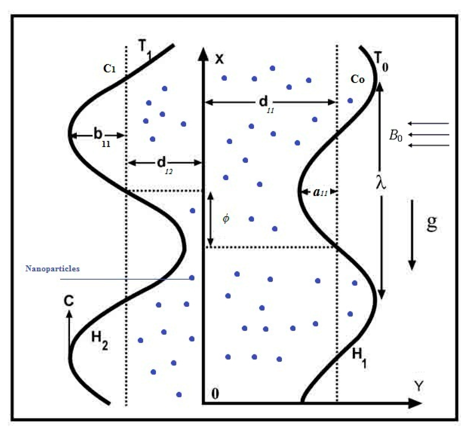
2. Mathematical Modeling

The incompressible Williamson model is chosen as a base fluid for nanofluid in between an asymmetric channel experiencing heat convection at the peristaltic type surfaces. The width of the channel is taken as $(d_{11}+d_{12})$. Flow is initiated due to the propagation of curved waves travelling with uniform speed $c$ towards the flow. The exchange of heat is recognized by imposing temperatures $T_0$ and $T_1$ at the lower and upper areas, correspondingly. To discuss nano particle phenomenon, we have taken the nanoparticle concentration $C_0$ and on the lower side and upper one, accordingly (see Figure 1).

The magnetic field $B_0$ is exerted orthogonally. The wall surfaces are taken as

$$Y=H_1=d_{11}+a_{11}\cos [2\pi \lambda X^{\prime }]$$

(1)

$$Y=H_2=-d_{12}-b_{11}\cos [2\pi \lambda X^{\prime }+\overline{\phi }], \mathrm{where} X^{\prime }=X-ct$$

(2)

In upper defined equations, $a_{11}$ and b₁₁ represent the wave amplitudes, λ gives the wavelength, $t$ suggests the time, $X$ depicts the wave’s direction, and $Y$ is placed normally to $X$. The range of phase variance $\overline{\phi }$ alters as $0\le \overline{\phi }\le \pi$. If $\overline{\phi }=0$, we meant that a symmetric dimensional channel is having waves located out of the phase and $\overline{\phi }=\pi$, suggest the waves within the phase. Moreover $a_{11}, b_{11}, d_{11}, d_{12}$ and $\overline{\phi }$ overcome the following relation

$$a_{11}^2+b_{11}^2+2a_{11}{b}_{11}\cos \overline{\phi }\le {(d_{11}+d_{12})}^2$$

(3)

The mathematical models of the considered problem given as

$$\mathbf{\nabla }\cdot \stackrel{⌢}{V}=0$$

(4)

$$\rho \left(\frac{\partial \stackrel{⌢}{V}}{\partial t}+\stackrel{⌢}{V}\cdot \mathbf{\nabla }\stackrel{⌢}{V}\right)=-\mathbf{\nabla }\overline{P}+\mathbf{\nabla }\cdot \mathbf{S}+{\rho }_f\mathbf{g}{\alpha }_f\left(\tilde{T}-T_0\right)+{\rho }_f\mathbf{g}{\alpha }_f\left(\tilde{C}-C_0\right)+\mathbf{J}\times \mathbf{B}$$

(5)

$${\left(\rho c\right)}_f\left(\frac{\partial \tilde{T}}{\partial t}+\stackrel{⌢}{V}\cdot \mathbf{\nabla }\tilde{T}\right)=\mathbf{\nabla }\cdot K\mathbf{\nabla }\tilde{T}+\mathbf{S}\cdot \mathbf{\nabla }\stackrel{⌢}{V}+{\left(\rho c\right)}_p\left(D_B\left(\mathbf{\nabla }\tilde{C}\cdot \mathbf{\nabla }\tilde{T}\right)+\frac{D_T}{T_m}(\mathbf{\nabla }\tilde{T}\cdot \mathbf{\nabla }\tilde{T})\right)$$

(6)

$$\frac{\partial \tilde{C}}{\partial t}+\widehat{V}\cdot \mathbf{\nabla }\tilde{C}=\mathbf{\nabla }\cdot \left(D_B\mathbf{\nabla }\tilde{C}+D_T\frac{\mathbf{\nabla }\tilde{T}}{T_o}\right)$$

(7)

where $\mathbf{g}$ is the gravitational body force and ${\alpha }_f$ represents the volumetric volume distension nanofluid’s coefficient. In above relations, ${(\rho c)}_f$ denotes the fluid’s heat capacity, ${(\rho c)}_p$ accounts for effective nanoparticles heat capacity, $\mathbf{J}=\sigma (\stackrel{⌢}{V}\times \overline{\mathbf{B}})$ reveals the current density, $\overline{\mathit{B}}=\left(0,B_0\right)$ notifies the external magnetic field, and $\mathbf{S}$ is placed for the Cauchy stress tensor for Williamson fluid and is determined as

$$\mathbf{\tau }=\left({\mu }_{\infty }+\left({\mu }_0+{\mu }_{\infty }\right) {\left(1-\mathsf{\Gamma }\stackrel{\cdot }{\mathbf{\gamma }}\right)}^{-1}\right) \stackrel{\cdot }{\overline{\mathbf{\gamma }}}$$

(8)

where $\stackrel{\cdot }{\overline{\mathbf{\gamma }}}$ comprises the subsequent value

$$\stackrel{\cdot }{\overline{\mathbf{\gamma }}}=\sqrt{\frac{1}{2}{\displaystyle \sum }_i{\displaystyle \sum }_j{\stackrel{\cdot }{\mathbf{\gamma }}}_{ij}{\stackrel{\cdot }{\mathbf{\gamma }}}_{ji}}=\sqrt{\frac{1}{2}\overline{\mathsf{\Pi }}}$$

(9)

Here $\overline{\mathsf{\Pi }}$ is the strain tensor. The velocity profile for the given problem is considered as $\stackrel{⌢}{V}=(U^{\prime }, V^{\prime }).$ Introducing a wavy frame we introduce the following transformations

$$x=X^{\prime }, y=Y, u=U^{\prime }-c, v=V^{\prime }, p(x)=\overline{P}(X, t)$$

(10)

We suggest the following dimensionless parameters to be used in the above expressions

$$\begin{array}{l}\overline{x}=\frac{2\pi x}{\lambda }, \overline{y}=\frac{y}{d_{11}}, \overline{u}=\frac{u}{c}, \overline{v}=\frac{v}{c\delta }, \delta =\frac{d_{11}}{\lambda }, d=\frac{d_{12}}{d_{11}}, \overline{p}=\frac{d_{11}^{2}p}{\mu c\lambda }, h_{11}=\frac{H_{11}}{d_{11}}, h_{12}=\frac{H_{12}}{d_{12}},\\ a_{12}=\frac{a_{11}}{d_{11}}, Br=Ec\mathrm{Pr}, b=\frac{b_{11}}{d_{11}}, \mathrm{Re}=\frac{\rho c{d}_{11}}{\mu }, \overline{\psi }=\frac{\psi }{c{d}_{11}}, \theta =\frac{\tilde{T}-T_0}{T_1-T_0}, Ec=\frac{c^2}{c_p(T_1-T_0)},\\ \mathrm{Pr}=\frac{\rho \nu c}{K}, \overline{S}=\frac{S{d}_{11}}{\mu c}, We=\frac{\mathsf{\Gamma }c}{d_{11}}, \phi =\frac{\tilde{C}-C_0}{C_1-C_0}, G_r=\frac{{\rho }_{f}g{\alpha }_f{d}^2\left(T_1-T_0\right)}{c\mu }, G_c=\frac{{\rho }_{f}g{\alpha }_f{d}^2\left(C_1-C_0\right)}{c\mu },\\ N_b=\frac{\tau D_B\left(C_1-C_0\right)}{\nu }, N_t=\frac{\tau D_T\left(T_1-T_0\right)}{\tau T_m},M=\sqrt{\frac{\sigma }{\mu }}{B}_0{d}_{11},We=\frac{\mathsf{\Gamma }c}{d_{11}}\end{array}$$

(11)

where $M,We,Br, \mathrm{Pr}, N_b, N_t, G_r$, and $G_c$ represent the Hartman number, Weissenberg number, Brinkman number, Prandtl number, Brownian motion parameter, thermophoresis parameter, local temperature Grashof number, and local nanoparticle Grashof number, accordingly. After incorporating the above structured parameters and applying the conditions of large wavelength along with small Reynolds number in a wavy frame coordinates we have the final form of Equations (4)–(7)

$$\begin{gathered} \frac{\partial u}{\partial x}+\frac{\partial v}{\partial y}=0 \\ \frac{dp}{dx}=\frac{\partial }{\partial y}\left[\frac{{\partial }^2\psi }{\partial y^2}-M^2\psi +We{\left(\frac{{\partial }^2\psi }{\partial y^2}\right)}^2\right]+G_r\theta +G_c\phi \end{gathered}$$

(12)

or

$$\frac{{\partial }^2}{\partial y^2}\left[\frac{{\partial }^2\psi }{\partial y^2}+We{\left(\frac{{\partial }^2\psi }{\partial y^2}\right)}^2-M^2\psi \right]+G_r\frac{\partial \theta }{\partial y}+G_c\frac{\partial \phi }{\partial y}=0$$

(13)

$$\mathrm{Pr}\left[N_b\frac{\partial \phi }{\partial y}\frac{\partial \theta }{\partial y}+N_t{\left(\frac{\partial \theta }{\partial y}\right)}^2\right]+\frac{{\partial }^2\theta }{\partial y^2}+Br\left[{\left(\frac{{\partial }^2\psi }{\partial y^2}\right)}^2+We{\left(\frac{{\partial }^2\psi }{\partial y^2}\right)}^3\right]=0$$

(14)

$$\frac{{\partial }^2\phi }{\partial y^2}+\frac{N_t}{N_b}\frac{{\partial }^2\theta }{\partial y^2}=0$$

(15)

where $\psi$ is stream function satisfying the relations u = ∂δ/∂y and $v=-\delta \partial \psi /\partial x,$ The no-slip boundary conditions for velocity u and nanoparticles fraction $\phi$ and convective boundaries are taken into consideration for temperature $\theta$ which have the following dimensionless form in the wave frame [15]

$$\begin{array}{c}\psi =\frac{F}{2}, \frac{\partial \psi }{\partial y}=-1, \mathrm{at} y=h_{11}, \psi =-\frac{F}{2}, \frac{\partial \psi }{\partial y}=-1, \mathrm{at} y=h_{12},\\ \frac{\partial \theta }{\partial y}-B_i\theta =-B_i \mathrm{at} y=h_{11} \mathrm{and} \theta =0 \mathrm{at} y=h_{12})\\ \phi =1 \mathrm{at} y=h_{11,} \mathrm{and} \phi =0 \mathrm{at} y=h_{12},\end{array}\}$$

(16)

where $h_{11}=1+a_{12}\cos x$ and $h_{12}=-d-b\cos (x+\phi ).$ Also $Bi=h_f{d}_{11}/K$ is the Biot number, $h_f$ stands for the coefficient of convective thermal transport. The mean flow rate in dimensionless format is elaborated as

$$Q=F+1+d$$

(17)

3. Solution of the Problem

The above obtained Equations (12)–(15) display the nonlinear ordinary differential equations in which $\psi$, $\theta$, and $\phi$ are mutually dependent. Such types of problems cannot be handled by exact techniques. Therefore, we chose a more appropriate solution procedure, the homotopy perturbation method (HPM) [16,17] to solve the current highly complicated boundary value problems. The deformation equations for $\psi$, $\theta$, and $\phi$ can be constructed as

$$\left(1-q^{\prime }\right){ℒ}_1\left(\widehat{\psi }-{\psi }_0\right)+q^{\prime }\left[\frac{{\partial }^2}{\partial y^2}\left(\frac{{\partial }^2\widehat{\psi }}{\partial y^2}+We{\left(\frac{{\partial }^2\widehat{\psi }}{\partial y^2}\right)}^2-M^2\widehat{\psi }\right)+G_r\frac{\partial \widehat{\theta }}{\partial y}+G_c\frac{\partial \widehat{\phi }}{\partial y}\right]= 0,$$

(18)

$$\left(1-q^{\prime }\right){ℒ}_2\left(\widehat{\theta }-{\theta }_0\right)+q^{\prime }\left[N_b\frac{\partial \widehat{\theta }}{\partial y}\frac{\partial \widehat{\phi }}{\partial y}+N_t{\left(\frac{\partial \widehat{\theta }}{\partial y}\right)}^2+\frac{{\partial }^2\widehat{\theta }}{\partial y^2}+Br{\left(\frac{{\partial }^2\widehat{\psi }}{\partial y^2}\right)}^2+We{\left(\frac{{\partial }^2\widehat{\psi }}{\partial y^2}\right)}^3\right]= 0,$$

(19)

$$\left(1-q^{\prime }\right){ℒ}_2\left(\widehat{\phi }-{\phi }_0\right)+q^{\prime }\left[\frac{{\partial }^2\widehat{\phi }}{\partial y^2}+\frac{N_t}{N_b}\frac{{\partial }^2\widehat{\theta }}{\partial y^2}\right]= 0,$$

(20)

where ${\pounds }_1$ and ${\pounds }_2$ are linear operators which are picked as $\pounds$

$${\pounds }_1=\frac{{\partial }^4}{\partial y^4} \mathrm{and} {\pounds }_2=\frac{{\partial }^2}{\partial y^2}$$

(21)

and $\stackrel{⌢}{{\psi }_0}$, $\stackrel{⌢}{{\theta }_0}$, and $\stackrel{⌢}{{\phi }_0}$ are the initial approximations which must satisfy the boundary conditions as well as differential operator. The initial approximations for $\psi , \theta , \mathrm{and} \phi$ are elected as

$$\stackrel{⌢}{{\psi }_0}=\frac{\left(h_{11}-h_{12}-2y\right) \left(-2\left(h_{11}-h_{12}\right) \left(h_{11}-y\right) \left(h_{12}-y\right)\right)}{2{(h_{11}-h_{12})}^2}+F\left(\frac{h_{11}^2-4h_{11}{h}_{12}+h_{12}^2+2\left(h_{11}+h_{12}\right) y-2y^2}{2{\left(h_{11}-h_{12}\right)}^2}\right)$$

(22)

$$\stackrel{⌢}{{\theta }_0}=\frac{B_i{h}_{12}-B_{i}y}{1-B_i{h}_{11}+B_i{h}_{12}}$$

(23)

$$\stackrel{⌢}{{\phi }_0}=\frac{-h_{12}+y}{h_{11}-h_{12}}$$

(24)

Applying perturbation on small embedding parameters $F\in [0, 1],$ we suggest the following series solutions

$$\stackrel{⌢}{\psi }={\psi }_0+q^{\prime }{\psi }_1+q^{\prime 2}{\psi }_2\dots$$

(25)

$$\stackrel{⌢}{\theta }={\theta }_0+q^{\prime }{\theta }_1+q^{\prime 2}{\theta }_2\dots$$

(26)

$$\stackrel{⌢}{\phi }={\phi }_0+q^{\prime }{\phi }_1+q^{\prime 2}{\phi }_2\dots$$

(27)

After substituting the above series solutions in Equations (18)–(20), we get the two systems for $\psi$, $\theta$, and $\phi$.

• Zeroth Order System

  $$\begin{array}{c}{\pounds }_1\left[{\psi }_0-\stackrel{⌢}{{\psi }_0}\right]=0,\\ {\psi }_0=\frac{F}{2}, \frac{\partial {\psi }_0}{\partial y}=-1, \mathrm{at} y=h_1, {\psi }_0=-\frac{F}{2}, \frac{\partial {\psi }_0}{\partial y}=-1, \mathrm{at} y=h_2,\end{array}\}$$

  (28)

  $$\begin{array}{c}{\pounds }_2\left[{\theta }_0-\stackrel{⌢}{{\theta }_0}\right]=0,\\ {\theta }_0\left(h_1\right)-B_i{\theta }_0\left(h_1\right)=-B_i \mathrm{at} y=h_i \mathrm{and} {\theta }_0=0 \mathrm{at} y=h_2\end{array}\}$$

  (29)

  $$\begin{array}{c}{\pounds }_2\left[{\phi }_0-\stackrel{⌢}{{\phi }_0}\right]=0,\\ {\phi }_0=1, \mathrm{at} y=h_1 \mathrm{and} {\phi }_0=0 \mathrm{at} y=h_2,\end{array}\}$$

  (30)
• First Order System

  $$\begin{array}{c}{\pounds }_1\left[\psi \right]+\frac{{\partial }^2}{\partial y^2}\left[\frac{{\partial }^2{\psi }_0}{\partial y^2}+We{\left(\frac{{\partial }^2{\psi }_0}{\partial y^2}\right)}^2-M^2{\psi }_0\right]+G_r\frac{\partial {\theta }_0}{\partial y}+G_c\frac{\partial {\phi }_0}{\partial y}=0,\\ {\psi }_1=0, \frac{\partial {\psi }_1}{\partial y}=0, \mathrm{at} y=h_1 \mathrm{and} {\psi }_1=0, \frac{\partial {\psi }_1}{\partial y}=0, \mathrm{at} y=h_{2,}\end{array}\}$$

  (31)

  $$\begin{array}{c}{\pounds }_2\left({\theta }_1\right)+N_b\left[\frac{\partial {\phi }_0}{\partial y}\cdot \frac{\partial {\theta }_0}{\partial y}\right]+N_t{\left(\frac{\partial {\theta }_0}{\partial y}\right)}^2+\frac{{\partial }^2{\theta }_0}{\partial y^2}+Br\left[{\left(\frac{{\partial }^2{\psi }_0}{\partial y^2}\right)}^2+We{\left(\frac{{\partial }^2{\psi }_0}{\partial y^2}\right)}^3\right]=0,\\ {\theta }_1^{\prime }\left(h_1\right)-B_i{\theta }_1\left(h_1\right)=0 \mathrm{at} y=h_1 \mathrm{and} {\theta }_1=0 \mathrm{at} y=h_2\end{array}\}$$

  (32)

  $$\begin{array}{c}{\pounds }_2\left({\phi }_1\right)+\frac{{\partial }^2{\phi }_0}{\partial y^2}+\frac{N_t}{N_b}\frac{{\partial }^2{\theta }_0}{\partial y^2}=0,\\ {\phi }_1=0, at y=h_1, {\phi }_1=0 at y=h_2,\end{array}\}$$

  (33)
• Zeroth Order Solutions
  By solving zeroth order systems by built-in technique in mathematical software, we obtain

  $$\begin{array}{c}{\psi }_0=\stackrel{⌢}{{\psi }_0}=\frac{\left(h_{11}+h_{12}-2y\right) \left(-2\left(h_{11}-h_{12}\right) \left(h_{11}-y\right) h_{12}-y\right)}{2\left(h_{11}-h_{12}\right)}+\\ \frac{F\left(h_{11}^2-4h_{11}{h}_{12}+h_{12}^2+2\left(h_{11}+h_{12}\right) y\right)-2y}{2{\left(h_{11}-h_{12}\right)}^2} \end{array}$$

  (34)

  $${\theta }_0=\stackrel{⌢}{{\theta }_0}=\frac{B_i{h}_2-B_{i}y}{1-B_i{h}_1+B_i{h}_2}$$

  (35)

  $${\phi }_0=\stackrel{⌢}{{\phi }_0}=\frac{-h_{12}+y}{h_{11}-h_{12}}$$

  (36)
• First Order Solutions
  The first order system has acquired the following general solutions

  $$\begin{array}{c}{\psi }_1=\frac{-1}{6\left(-1+B_i{\left(h_{11}-h_{12}\right)}^7\right)}[1/4G_c{\left(-1+B_i(h_{11}-h_{12}\right)}^6-6\left(F+h_{11}-h_{12}\right)(-h_{11}{M}^2+2h_{11}^3\\ h_{12}{M}^2-2h_{11}{h}_{12}^3{M}^2+h_{12}^4{M}^2+48We\left(F+h_{11}-h_{12}\right)+B_i\left(h_{11}-h_{12}\right)(G_r{\left(h_{11}-h_{12}\right)}^5+\\ 6\left(F+h_{11}-h_{12}\right) \left(-h_{11}^4{M}^2+2h_{11}^3{h}_{12}{M}^2++h_{12}^4{M}^2+48We\left(F+h_{11}-h_{12}\right)\right)))y^4+\\ \frac{3}{5}\left(-1+B_i{\left(h_{11}-h_{12}\right)}^4\left(F+h_{11}-h_{12}\right) M^2{y}^5\right)]+L_{11}+y{L}_{12}+y^2{L}_{13}+y^3{L}_{14}\end{array}$$

  (37)

  $$\begin{array}{c}{\theta }_1=\frac{1}{{\left(-1+B_i\left(h_{11}-h_{12}\right)\right)}^2{\left(h_{11}-h_{12}\right)}^9}[1/2B_i{\left(h_{11}-h_{12}\right)}^8(\left(-1+B_i\left(h_{11}-h_{12}\right)\right) N_b+\\ B_i\left(h_{11}-h_{12}\right) N_t)\mathrm{Pr}+36Br(-1+B_i{\left(h_{11}-h_{12})\right)}^2{\left(F+h_{11}-h_{12}\right)}^2{\left(h_{11}-h_{12}\right)}^2(h_{11}^3-\\ 3h_{12}^2(h_{12}-2We)+3h_{11}\left(h_{12}^2+2FWe\right)-h_{12}\left(h_{12}^2-6We+6h_{12}We\right)))y^2-24Br\\ {\left(-1+B_i\left(h_{11}-h_{12}\right)\right)}^2{\left(F+h_{11}-h_{12}\right)}^2\left(h_{11}+h_{12}\right) h_{11}^3-3h_{11}^2\left(h_{12}-3We\right)+3h_{12}\\ \left(h_{12}^2+3FWe\right)(-h_{12}(h_{12}^2-9FWe+9h_{12}We))y^3+12Br(-1+B_i\left(h_{11}-h_{12}\right){)}^2(F+\\ h_{11}-h_{12}{)}^2(h_{11}^3-3h_{11}^2\left(h_{12}-6We\right)+3h_{11}\left(h_{12}^2+6FWe\right)-h_{12}(h_{12}^2-18FWe+18\\ h_{12}We))y^4)]-\frac{432}{5}Br{\left(-1+B_i\left(h_{11}-h_{12}\right) {\left(F+h_{11}-h_{12}\right)}^2\right)}^{3}We{y}^5+L_{15}+y{L}_{16} \end{array}$$

  (38)

  $$\begin{array}{c}{\phi }_1=\frac{1}{{\left(-1+B_i\left(h_{11}-h_{12}\right)\right)}^2{\left(h_{11}-h_{12}\right)}^9{N}_b}{N}_t[1/3B_i{\left(h_{11}-h_{12}\right)}^8(\left(-1+B_i\left(h_{11}-h_{12}\right)\right) N_b+\\ B_i\left(h_{11}-h_{12}\right) N_t)\mathrm{Pr}+36Br{\left(-1+B_i\left(h_{11}-h_{12}\right)\right)}^2{\left(F+h_{11}-h_{12}\right)}^2{\left(h_{11}-h_{12}\right)}^2(h_{11}^3\\ -3h_{11}^2\left(h_{12}-2We+3h_1\left(h_{12}^2+2FWe\right)-h_{12}\left(h_{12}^2-6FWe+6h_{12}We\right)\right))Y^2-24Br(-1\\ +B_i\left(h_{11}-h_{12}\right){)}^2{\left(F+h_{11}-h_{12}\right)}^2\left(h_{11}+h_{12}\right) h_{11}^3-3h_{12}^2\left(h_{12}-3We\right)+h_{11}\left(h_{12}^2+3FWe\right) \\ \left(-h_{12}\left(h_{12}^2-9FWe\right)+9h_{2}We\right) Y^3+12G_c(-1+B_i{\left(h_{11}-h_{12}\right)}^2{\left(F+h_{11}-h_{12}\right)}^2\\ \left(h_{11}^3-3h_{11}^2\left(h_{12}-6We\right)+3h_{11}^2\left(h_{12}-6We\right)+3h_{11}\left(h_{11}^2+6FWe\right)-h_{12}\left(h_{12}^2-18FWe\right)\right) \\ y^4]-{\left(\frac{432}{5}Br{\left(-1+B_i\left(h_{11}-h_{12}\right)\right)}^2{\left(F+h_{11}-h_{12}\right)}^2\right)}^{3}We{y}^5+L_{17}+y{L}_{18}\end{array}$$

  (39)

The final solutions according to the concept of HPM are given by using q → 1 in Equations (2)–(27).

$$\psi ={\psi }_0+{\psi }_1+\dots$$

(40)

$$\theta ={\theta }_0+{\theta }_1+\dots$$

(41)

$$\phi ={\phi }_0+{\phi }_1+\dots$$

(42)

where constants $L_{ij},$ $i=1, j=1-8$ can be found by routine calculation. The complete solutions of $\psi$, $\theta$, and $\phi$ can be obtained by supposed solutions. The solution for pressure gradient $dp/dx$ can be found by simply substituting the values in Equation (12). The mathematical formula for the pressure increase function $∆p$ can been visualized in next equation that has been solved numerically by built-in technique numerical integration on Mathematica.

$$∆p=\underset{0}{\overset{1}{{\displaystyle \int }}}\left(\frac{dp}{dx}\right) dx$$

(43)

4. Results and Discussion

This portion comprises of graphical results and discussion of obtained results for velocity, temperature, nanoparticles, pressure gradient, and stream functions. The numerical data of the pressure rise function $∆p$ is also sketched against the domain of flow rate and found the effects of physical parameters separately. Figure 2 and Figure 3 are sketched for the velocity profile with varying the values of $(G_r)$ and $(G_c)$, respectively in corresponding order. From Figure 2, it is clearly visible that velocity is decreasing in lower part and increasing in upper part of the channel and enhances its maximum peak at the center under the effect of $G_r$. One can see the similar behavior by taking increasing values of $G_c$ but here the difference is that the velocity is not varying much under the effect of $G_c$ in Figure 3. Figure 4, Figure 5 and Figure 6 contain correspondingly the alteration of temperature profile $\theta$ with the variability of Biot number $(B_i)$, Brinkman number $(Br)$, and the Prandtl number $(\mathrm{Pr}).$ From Figure 4, one can notice that the temperature profile is stretched vertically with the increase in magnitudes of $B_i$. It depicts that heat convection at the boundaries enhances the temperature of the Williamson nanofluid. It is also notable here that the temperature is maximum at lower wall and minimum at the lower surface and there is much variation in temperature level at upper region as compared to lower side. Figure 5 reflects the observation that temperature is an increasing function of $Br$ and the temperature gradients are prominent at the lower portions as equated with the upper ones, but the extent of heat is similar at both the surfaces as was observed for $B_i$. It can be received from Figure 6 that temperature profile is increasing in linear fashion for numerically increasing magnitudes of $Pr$ but the change in heat is calculated more significantly in the central parts of the enclosure which is the totally different result than we have achieved in Figure 4 and Figure 5. Figure 7 and Figure 8 are presented to see the behavior of nanoparticles volume fraction $\phi$ with increasing magnitudes of $(N_b)$ and $(N_t)$. Figure 7 shows that $\phi$ is getting higher when someone increases $N_b$. It is also explicit here that nanoparticles are dispersed in the region between the lower and upper surfaces. On the other hand, Figure 8 revels different story, the increase in $N_t$ decreases the nanoparticles concentration. Figure 9 is plotted for pressure gradient $dp/dx$ for $N_b.$ It is seen that $dp/dx$ is increasing as we increase $N_b$ and gets maximum height at the center of the domain, i.e., $x=0.5$. From Figure 10, we can see that pressure gradient is varying quite opposite manner for the parameter $N_t$. It can also be noticed from Figure 9 and Figure 10 that pressure gradient gets positive values only in the central part and remains negative at the corners. Figure 11 and Figure 12 are displaced to see the effects of parameters $M$ and $We$ on pressure rise $∆p$. Here the whole area is broken into three zones, namely Region I–III. The Region I is recognized by the portion where $Q>0, ∆p>0$. Region II is named the place where $Q>0$ and $∆p<0$ while Region III is composed of the part $Q, ∆p<0$. Figure 11 shows that $∆p$ curves are increasing in Region I and II while decreasing in Region III with the variation of $M$. Also, the free pumping exists at $Q\approx 1.5$. In Figure 12, it is observed that in Region I and II, $∆p$ is increasing and in Region III, it is decreasing. Also, the peristaltic pumping occurs in Regions I and II between the interval $(-1.7, 0.5)$. The streamlines are drawn in Figure 13, Figure 14 and Figure 15 for the parameters $G_c$, $We$, and $M$, respectively. From Figure 13, it is clear that the number of boluses is increasing, but size of the trapped bolus is decreasing in lower part of the channel, while in upper portion, the situation is totally reflected in opposite ways. Figure 14 gives the streamlines variation under the different values of $We$. It is attained here that, in the lower part, the number of boluses is increasing but size is changing randomly. The stream function for $M$ has been sketched in Figure 15 and it is noted in both the lower and upper parts, the size of bolus in increasing while number is decreasing. It is also admitted by Figure 13, Figure 14 and Figure 15 that trapped boluses are displaced towards left from upper to lower side due to asymmetric dimensions of the channel which can be made symmetric by imposing $\overline{\phi }=0.$

5. Conclusions

In this article, the authors have discovered the mathematical treatment of the peristaltic flow of Williamson nanofluid coated with the walls of an asymmetric heated channel. The flow has been studied analytically and graphically through variation of some pertinent parameters. From the above discussion, the main findings are given below:

(1)

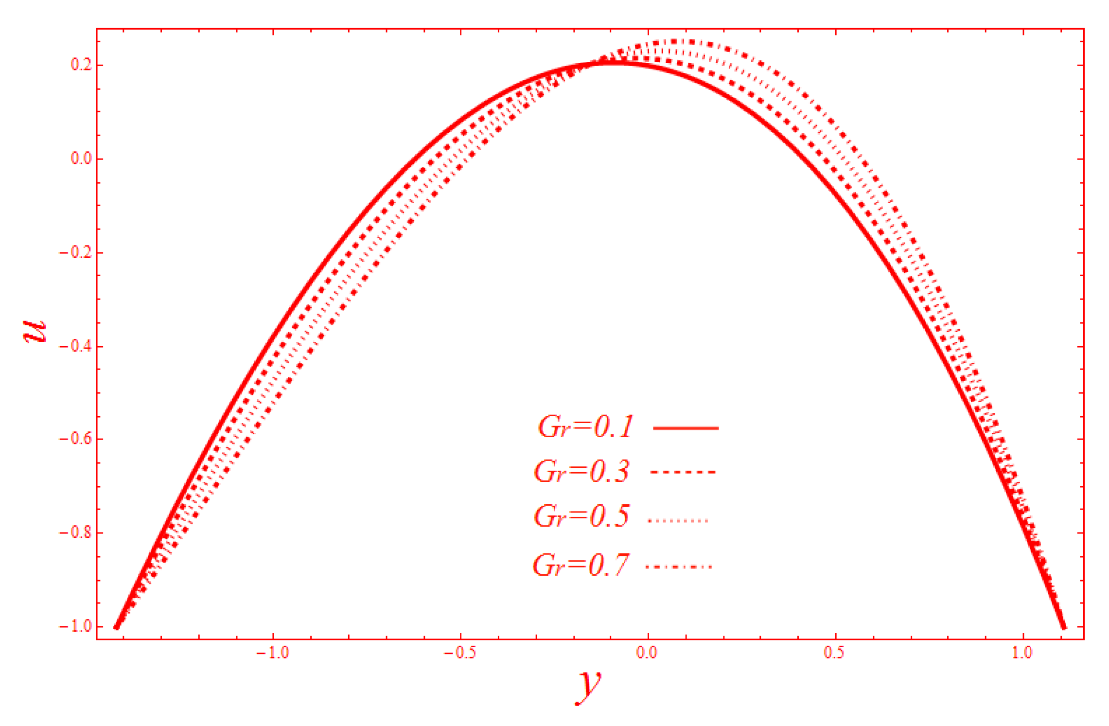
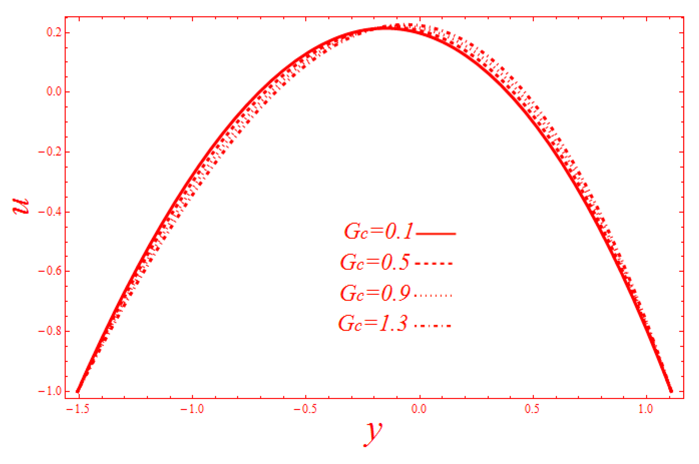
The velocity of nanofluid is decreasing in the lower part while increasing in the upper side with local temperature Grashof number and local nanoparticle Grashof number.

(2)

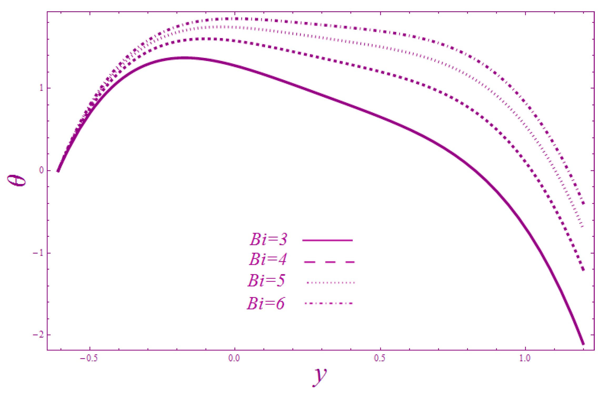
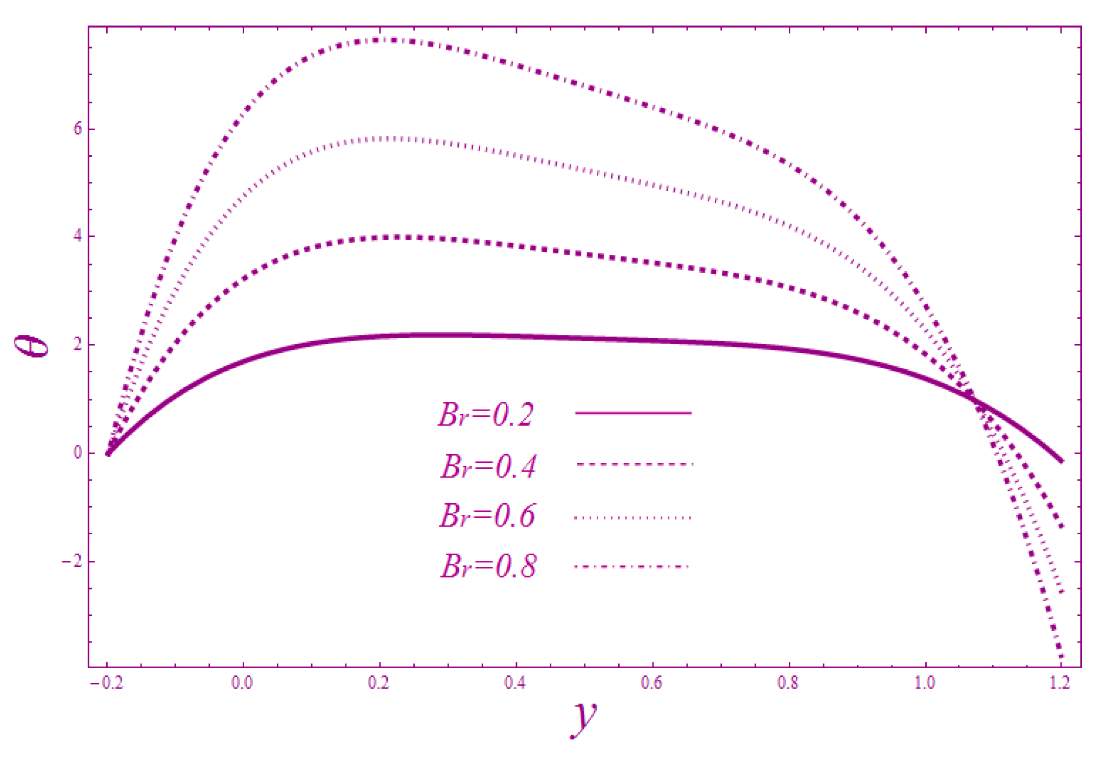
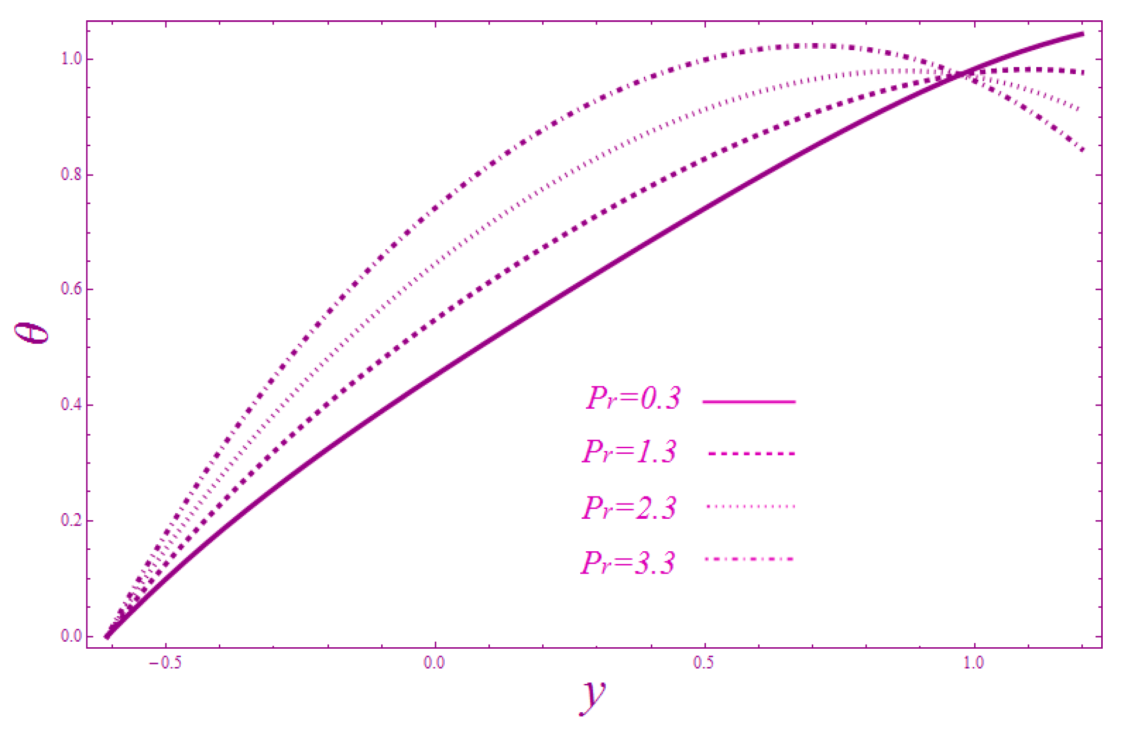
The temperature is becoming large with an increase in Biot number, Brinkman number, and Prandtl number.

(3)

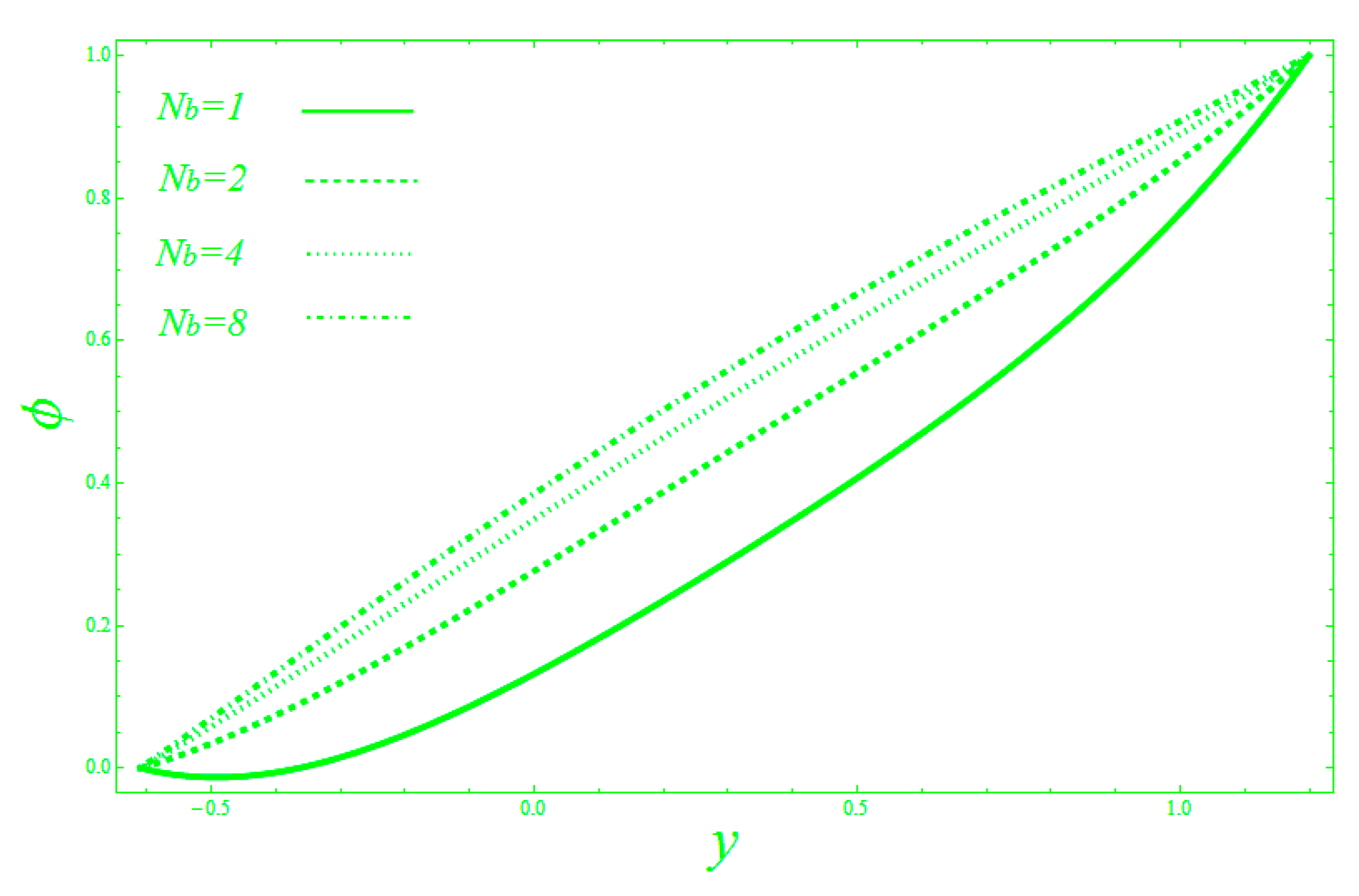
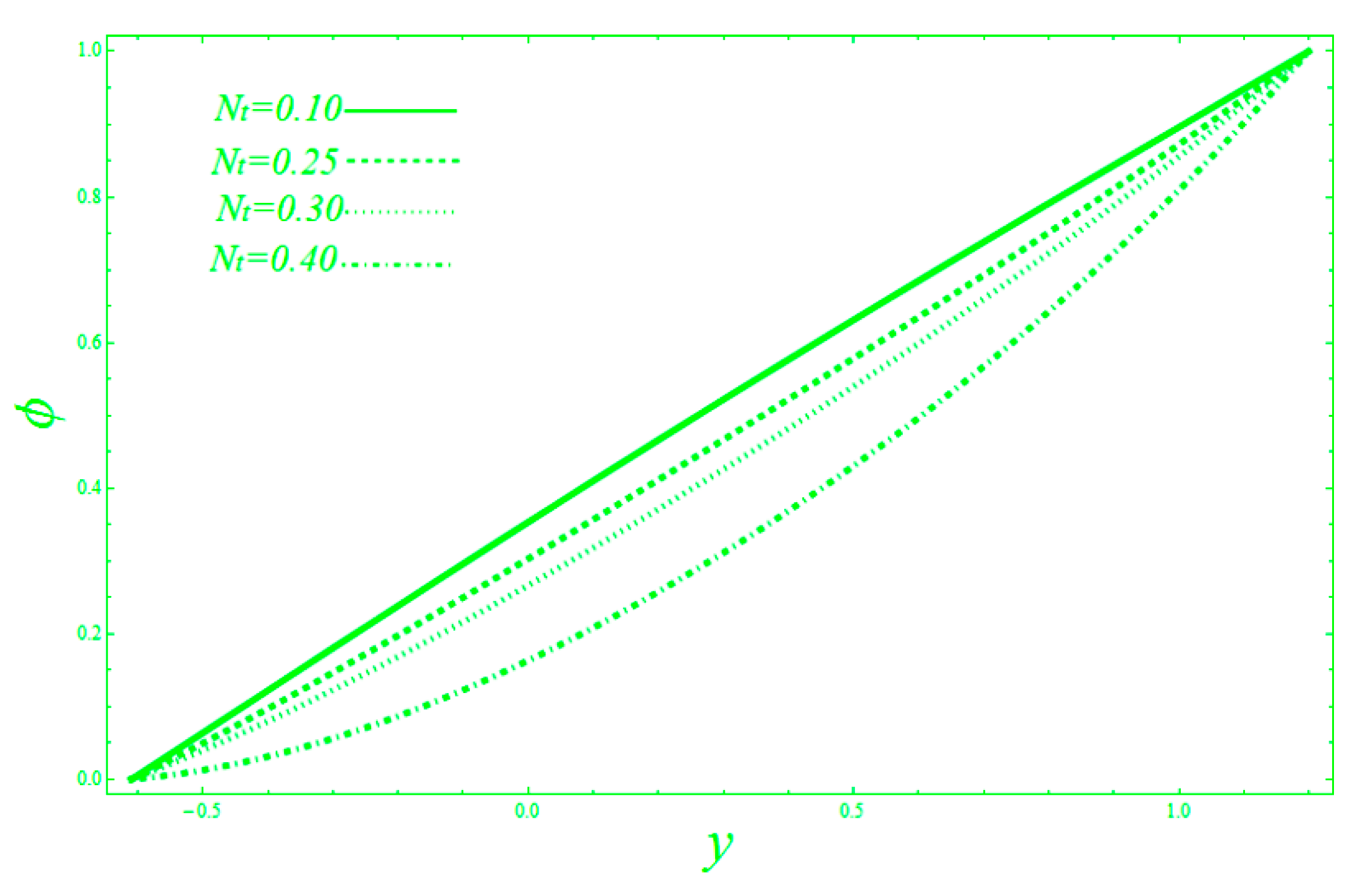
The nano particle concentration is getting higher when we increase Brownian motion parameter, but diminishes with thermophoresis parameter.

(4)

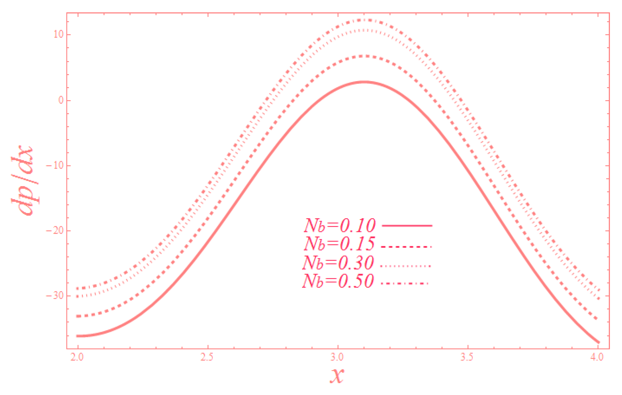
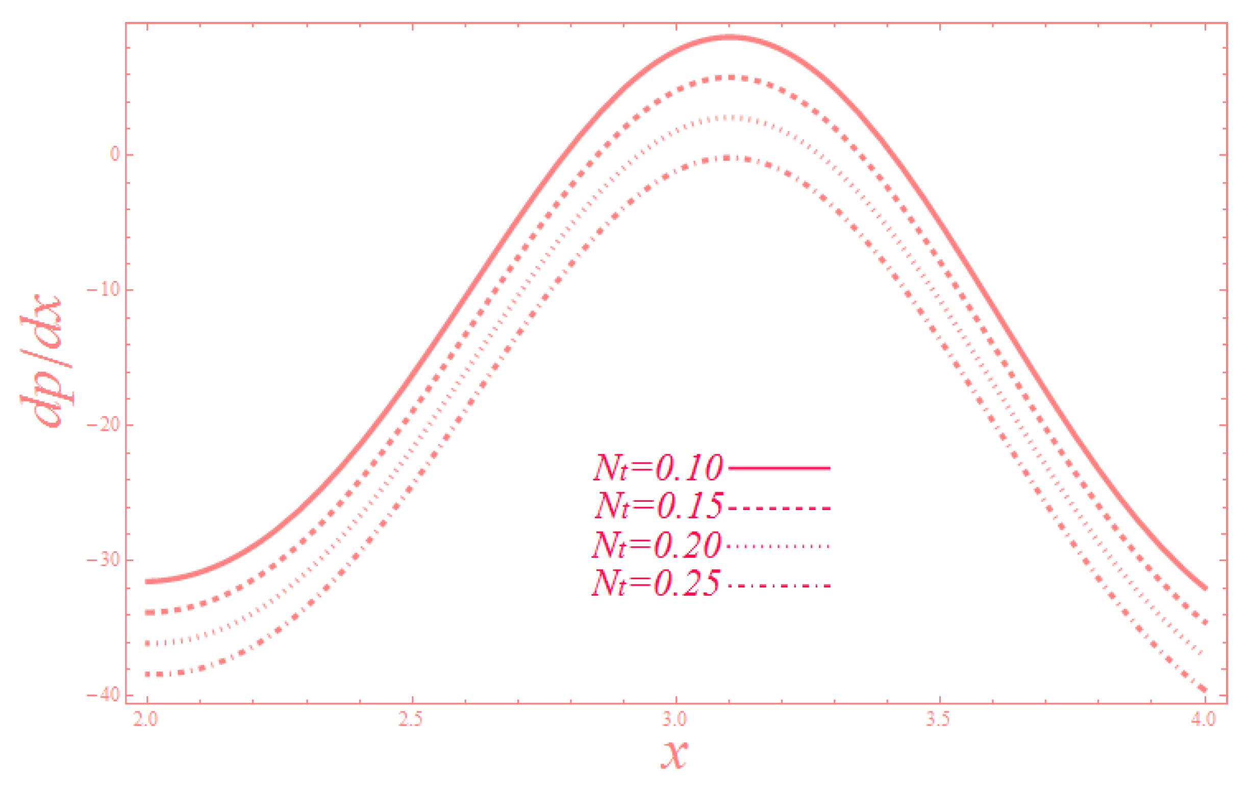
The pressure gradient is increasing with Brownian motion parameter, but lessening for thermophoresis parameter.

(5)

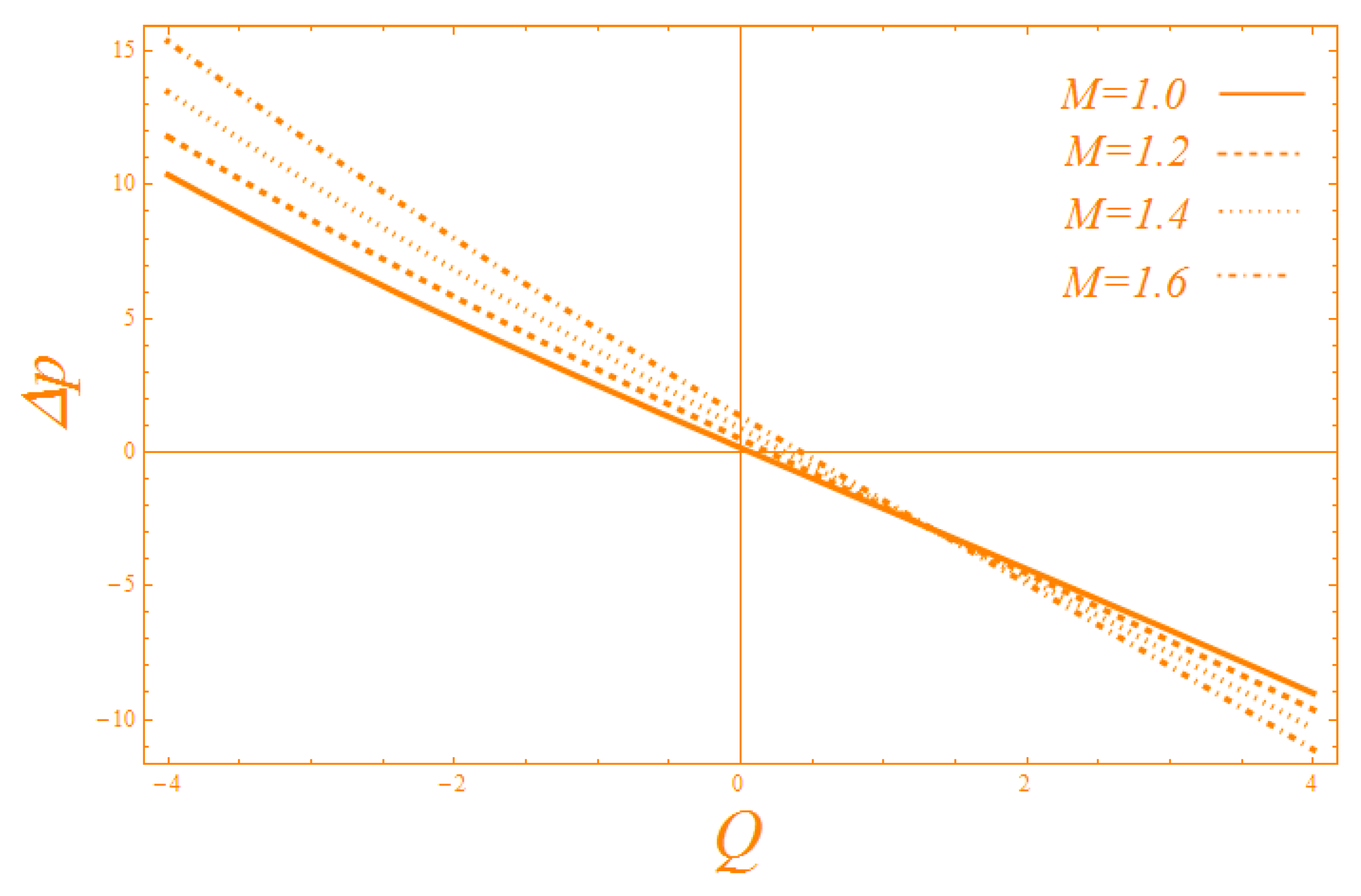
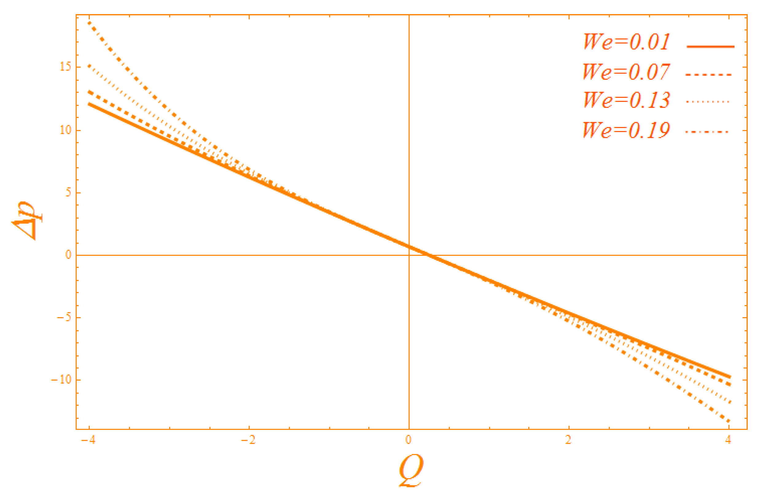
The peristaltic pumping fasten up with Hartman number and Weissenberg number.

(6)

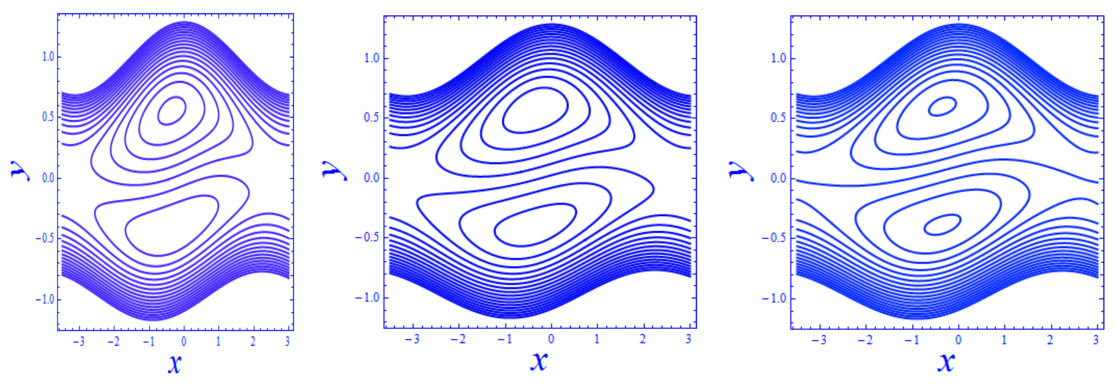
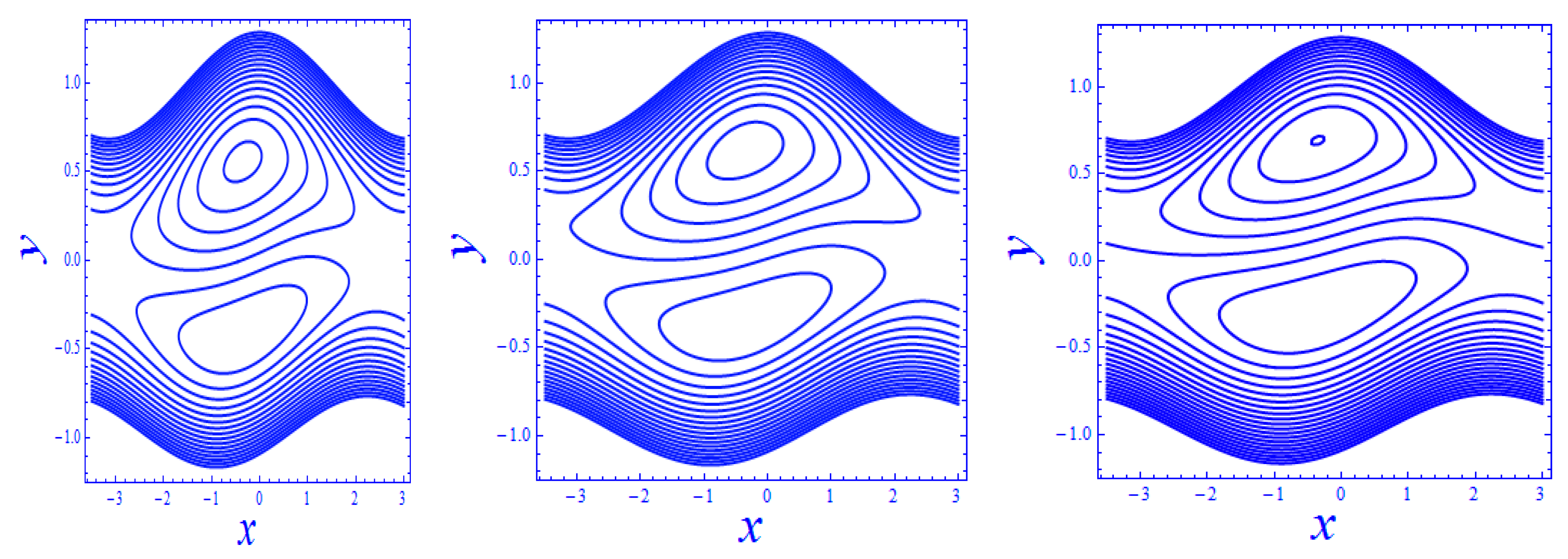
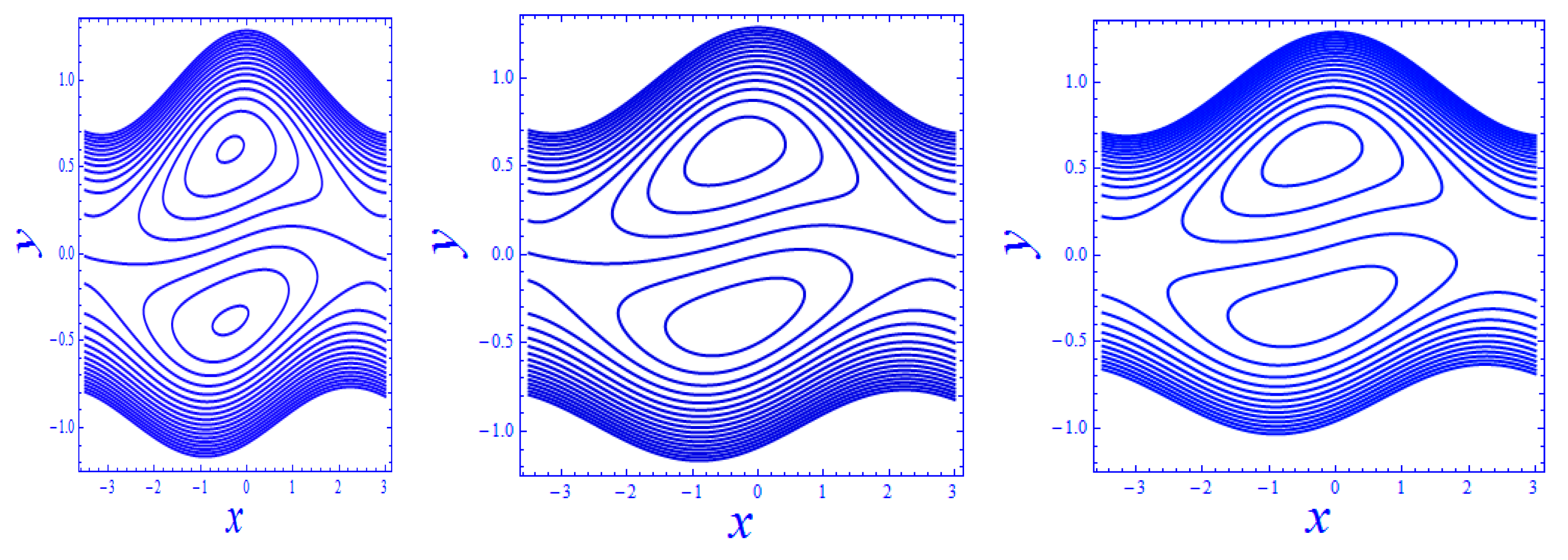
In the upper portion, the size of the trapped bolus is decreasing, but increasing in lower portion when we increase local nanoparticle Grashof numbers and Weissenberg numbers, but it varies in a random manner with Hartman numbers.

(7)

It is important to notice that boluses are trapped by their position in lower and upper corners of the channel due to its asymmetric structure. We can recover the results of symmetric channel by neglecting the phase difference.

(8)

The study of viscous nanofluid can be approached by neglecting Weissenburg number.

References

1. Maxwell, J.C. A Treatise on Electricity and Magnetism, 2nd ed.; Clarendan Press: Oxford, UK, 1881. [Google Scholar]
2. Choi, S.U.S.; Eastman, J.A. Enhancing Thermal Conductivity of Fluids with Nanoparticles; Argonne National Lab: Du Page County, IL, USA, 1995. [Google Scholar]
3. Hassan, M.; Marin, M.; Alsharif, A.; Ellahi, R. Convective heat transfer flow of nanofluid in a porous medium over wavy surface. Phys. Lett. A 2018, 382, 2749–2753. [Google Scholar] [CrossRef]
4. Safaei, M.R.; Togun, H.; Vafai, K.; Kazi, S.N.; Badarudin, A. Investigation of heat transfer enhancement in a forward-facing contracting channel using FMWCNT nanofluids. Numer. Heat Transf. Part A Appl. 2014, 66, 1321–1340. [Google Scholar] [CrossRef]
5. Alsagri, A.S.; Nasir, S.; Gul, T.; Islam, S.; Nisar, K.S.; Shah, Z.; Khan, I. MHD Thin Film Flow and Thermal Analysis of Blood with CNTs Nanofluid. Coatings 2019, 9, 175. [Google Scholar] [CrossRef]
6. B’eg, O.A.; Tripathi, D. Mathematica simulation of peristaltic pumping with double-diffusive convection in nanofluids: A bio-nano-engineering model. J. Nanoeng. Nanosyst. 2011, 225, 99–114. [Google Scholar]
7. Akbar, N.S.; Maraj, E.N.; Butt, A.W. Copper nanoparticles impinging on a curved channel with compliant walls and peristalsis. Eur. Phys. J. Plus. 2014, 129, 183. [Google Scholar] [CrossRef]
8. Bhatti, M.M.; Rashidi, M.M. Effects of thermo-diffusion and thermal radiation on Williamson nanofluid over a porous shrinking/stretching sheet. J. Mol. Liq. 2016, 221, 567–573. [Google Scholar] [CrossRef]
9. Bhatti, M.M.; Sheikholeslami, M.; Zeeshan, A. Entropy analysis on electro kinetically modulated peristaltic propulsion of magnetized nanofluid flow through a microchannel. Entropy 2017, 19, 481. [Google Scholar] [CrossRef]
10. Prakash, J.; Tripathi, D.; Tiwari, A.K.; Sait, S.M.; Ellahi, R. Peristaltic Pumping of Nanofluids through a Tapered Channel in a Porous Environment: Applications in Blood Flow. Symmetry 2019, 11, 868. [Google Scholar] [CrossRef]
11. Aziz, A. A similarity solution for laminar thermal boundary layer over a flat plate with a convective surface boundary condition. Commun. Nonlinear Sci. Numer. Simul. 2009, 14, 1064–1068. [Google Scholar] [CrossRef]
12. Makinde, O.D.; Aziz, A. MHD mixed convection from a vertical plate embedded in a porous medium with a convective boundary condition. Int. J. Therm. Sci. 2010, 49, 1813–1820. [Google Scholar] [CrossRef]
13. Makinde, O.D. Similarity solution of hydromagnetic heat and mass transfer over a vertical plate with a convective surface boundary condition. Int. J. Phys. Sci. 2010, 5, 700–710. [Google Scholar]
14. Merkin, J.H.; Pop, I. The forced convection flow of a uniform stream over a flat surface with a convective surface boundary condition. Commun. Nonlinear Sci. Numer. Simul. 2011, 16, 602–3609. [Google Scholar] [CrossRef]
15. Akbar, N.S. Non-Newtonian fluid flow in an asymmetric channel with convective surface boundary condition: A note. J. Power Technol. 2014, 94, 34–41. [Google Scholar]
16. He, J.H. Homo topy perturbation method for solving boundary value problems. Phys. Lett. A 2006, 350, 87–88. [Google Scholar] [CrossRef]
17. He, J.H. Homotopy perturbation method: A new nonlinear analytical technique. Appl. Math. Comput. 2003, 135, 73–79. [Google Scholar] [CrossRef]
Figure 1. Geometry of the channel.
Coatings 09 00816 g001
Figure 2. Modification of velocity profile against G r for x = 1 ,   F = 2 ,   a = 0.2 ,   b = 0.1 ,   d = 1.5 ,   φ = 1.5 ,   G c = 0.3 ,   W e = 0.01 ,   M = 0.1 ,   B i = 0.5 .
Coatings 09 00816 g002
Figure 3. Modification of velocity profile against G c for x = 1 ,   F = 2 ,   a = 0.2 ,   b = 0.1 ,   d = 1.5 ,   φ = 1.5 ,   G r = 0.1 ,   W e = 0.01 ,   M = 0.1 ,   B i = 0.5 .
Coatings 09 00816 g003
Figure 4. Modification of temperature profile against B i for, n = 2 ,   x = 0.1 ,   F = 5 ,   a = 0.2 ,   b = 0.1 ,   d = 0.51 ,   φ = 0.01 ,   W = 0.01 ,   M = 0.1 ,   G c = 0.9 ,   G r = 4 ,   G c = 0.3 ,   N b = 0.5 ,   Pr = 0.4 ,   N t = 0.2 .
Coatings 09 00816 g004
Figure 5. Modification of temperature profile against B r for n = 2 ,   x = 0.1 ,   F = 5 ,   a = 0.2 ,   b = 0.1 ,   d = 0.1 ,   φ = 0.1 ,   W e = 0.01 ,   G c = 0.9 ,   G r = 1 ,   B i     = 10 ,   N b = 0.5 ,   Pr = 0.4 ,   N t = 0.2 .
Coatings 09 00816 g005
Figure 6. Modification of temperature profile against Pr for n = 2 ,   x = 0.1 ,   F = 5 ,   a = 0.2 ,   b = 0.1 ,   d = 0.51 ,   φ = 0.1 ,   W e = 0.01 ,   G c = 0.9 ,   G r = 1 ,   B i     = 5 ,   N b = 0.5 ,   G c = 0.01 ,   N t = 0.2 .
Coatings 09 00816 g006
Figure 7. Modification of nanoparticles concentration against N b for n = 2 ,   x = 0.1 ,   F = 5 ,   a = 0.2 ,   b = 0.1 ,   d = 0.51 ,   φ = 0.01 ,   W e = 0.01 ,   G c = 0.9 ,   G r = 4 ,   B i     = 0.5 ,   Pr = 0.4 ,   G c = 0.1 ,   N t = 0.2 .
Coatings 09 00816 g007
Figure 8. Modification of nanoparticles concentration against N t for, n = 2 ,   x = 0.1 ,   F = 2 ,   a = 0.2 ,   b = 0.1 ,   d = 0.51 ,   φ = 0.01 ,   W e = 0.01 , , G c = 0.9 ,   G r = 4 ,   B i = 0.5 ,   Pr = 0.4 ,   G c = 0.1 ,   N t = 0.2 .
Coatings 09 00816 g008
Figure 9. Modification of pressure gradient against N b for n = 2 ,   y = 0.1 ,   F = 10 ,   a = 0.2 ,   b = 0.1 ,   d = 0.51 ,   φ = 0.01 , W e = 0.1 ,   G c = 0.9 ,   G r = 4 ,   B i     = 0.5 ,   Pr = 0.4 ,   G c = 0.1 ,   M = 1.5 ,   N t = 0.2 .
Coatings 09 00816 g009
Figure 10. Modification of pressure gradient against N t for, n = 2 ,   y = 0.1 ,   F = 10 ,   a = 0.2 ,   b = 0.1 ,   d = 0.51 ,   φ = 0.01 ,   W e = 0.1 , , G c = 0.9 ,   G r = 4 ,   B i     = 0.09 ,   Pr = 0.4 ,   G c = 0.3 ,   M = 1.5 ,   N b = 0.1 .
Coatings 09 00816 g010
Figure 11. Modification of pressure rise against M for, n = 2 ,   y = 0.1 ,   F = 10 ,   a = 0.2 ,   b = 0.3 ,   d = 0.5 ,   φ = 0.01 ,   M = 1.3 ,   G c = 0.3 ,   G r = 0.1 ,   B i     = 0.3 ,   Pr = 0.4 ,   G c = 0.3 ,   N b = 0.3 ,   N t = 0 .
Coatings 09 00816 g011
Figure 12. Modification of pressure rise against W e for, n = 0.1 ,   y = 0.1 ,   a = 0.2 ,   b = 0.3 ,   d = 0.5 ,   φ = 0.01 ,   M = 1.3 ,   G c = 0.3 ,   G r = 0.1 ,   B i     = 0.3 ,   Pr = 0.4 ,   G c = 0.3 ,   N b = 0.3 ,   N t = 0.2 .
Coatings 09 00816 g012
Figure 13. Modification of streamlines for G c = { 0.1 , 0.5 , 0.9 } when n = 0.1 ,   y = 0.1 ,   F = 5 ,   a = 0.3 ,   b = 0.2 ,   d = 0.1 ,   φ = 0.01 ,   M = 0.1 ,   W e = 0.1 ,   G r = 4 ,   B i     = 0.09 ,   Pr = 0.4 ,   B r = 0.9 ,   N b = 0.5 ,   N t = 0.2 .
Coatings 09 00816 g013
Figure 14. Modification of streamlines for W e = { 0.1 , 0.2 , 0.3 } when n = 0.1 ,   y = 0.1 ,   a = 0.2 ,   b = 0.3 ,   d = 0.5 ,   φ = 0.01 ,   M = 0.1 ,   B i     = 0.09 ,   Pr = 0.4 ,   G c = 0.9 ,   G r = 4 ,   N b = 0.5 ,   N t = 0.2 .
Coatings 09 00816 g014
Figure 15. Modification of streamlines for M = { 0.1 , 0.9 , 1.7 } when n = 2 ,   F = 5 ,   a = 0.3 ,   b = 0.2 ,   d = 1 ,   φ = 0.01 ,   W e = 0.1 ,   G r = 4 ,   G c = 0.1 ,   B i     = 0.09 ,   Pr = 0.4 ,   G c = 0.9 ,   N b = 0.5 ,   N t = 0.2 .
Coatings 09 00816 g015