Figure 1.
Tecsis Model Selection Tool (MST) main window.
Figure 1.
Tecsis Model Selection Tool (MST) main window.
Figure 2.
Structure of neural network in the present work.
Figure 2.
Structure of neural network in the present work.
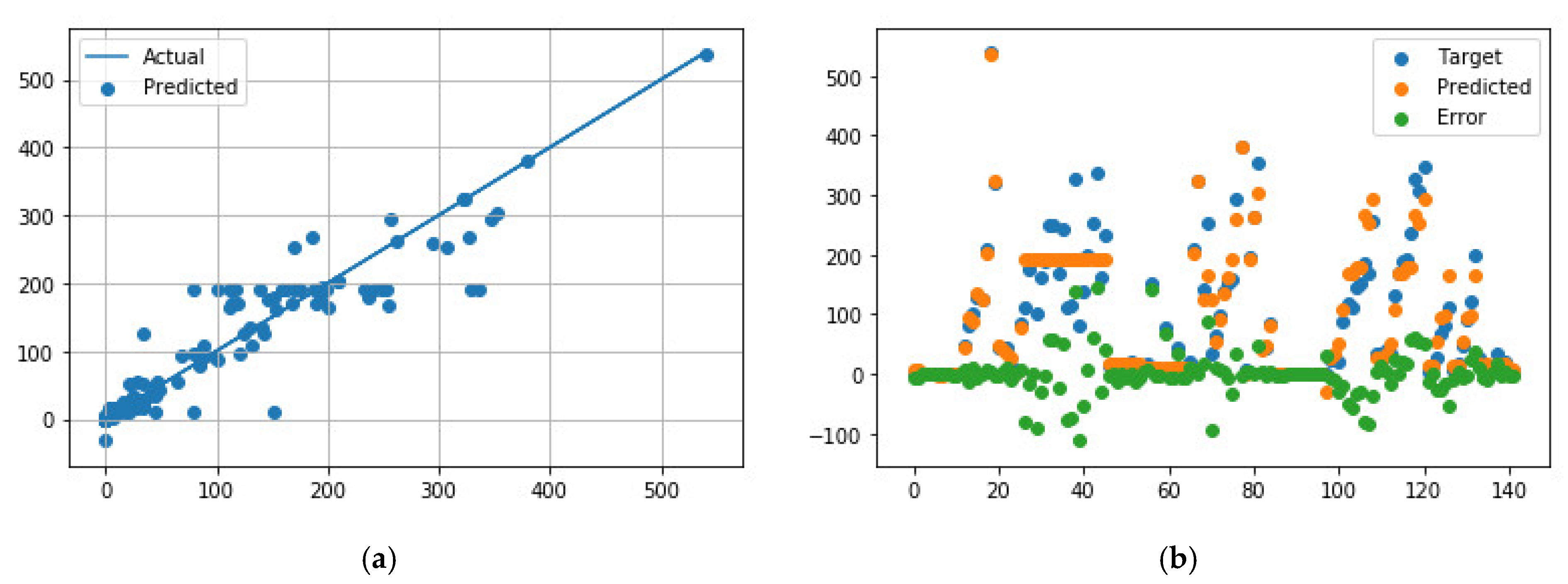
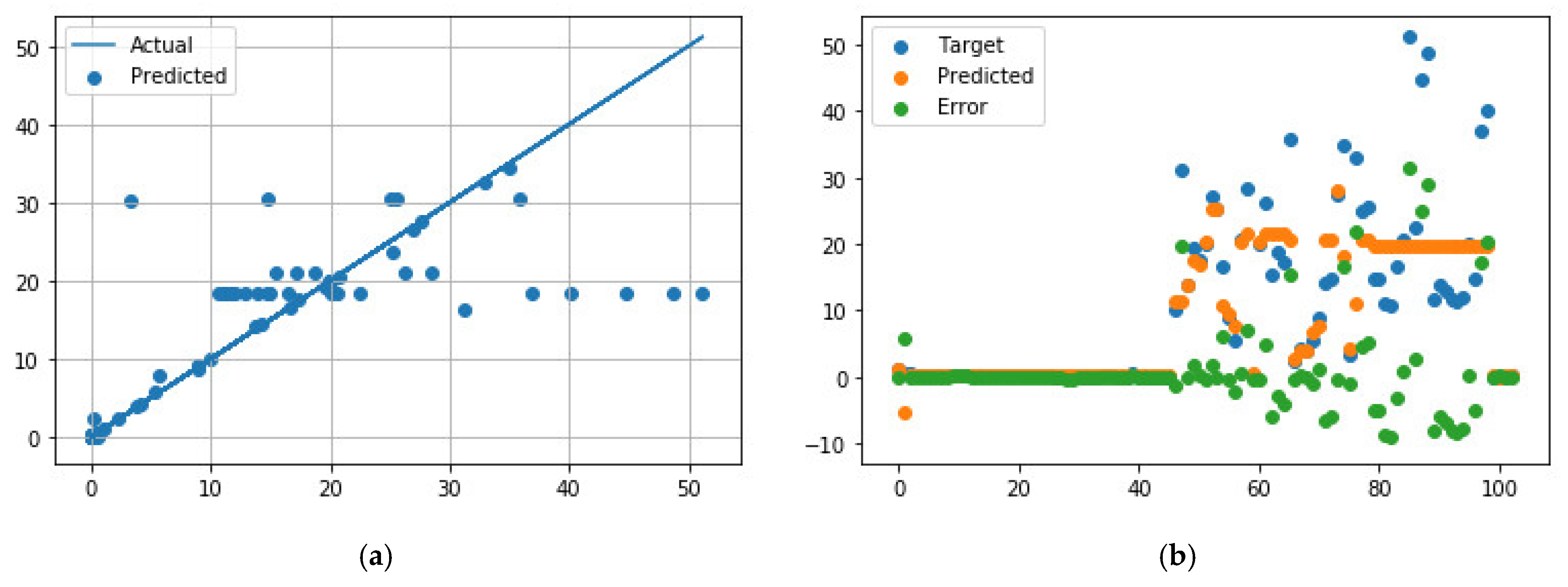
Figure 3.
Comparison of predicted and measured ER values for APS + EB-PVD data points using the best NN model parameters. (a) Predicted values vs. actual values; (b) Distribution of actual values, predicted values, and errors.
Figure 3.
Comparison of predicted and measured ER values for APS + EB-PVD data points using the best NN model parameters. (a) Predicted values vs. actual values; (b) Distribution of actual values, predicted values, and errors.
Figure 4.
Comparison of predicted and measured ER values for APS data points using the best NN model parameters. (a) Predicted values vs. actual values; (b) Distribution of actual values, predicted values, and errors.
Figure 4.
Comparison of predicted and measured ER values for APS data points using the best NN model parameters. (a) Predicted values vs. actual values; (b) Distribution of actual values, predicted values, and errors.
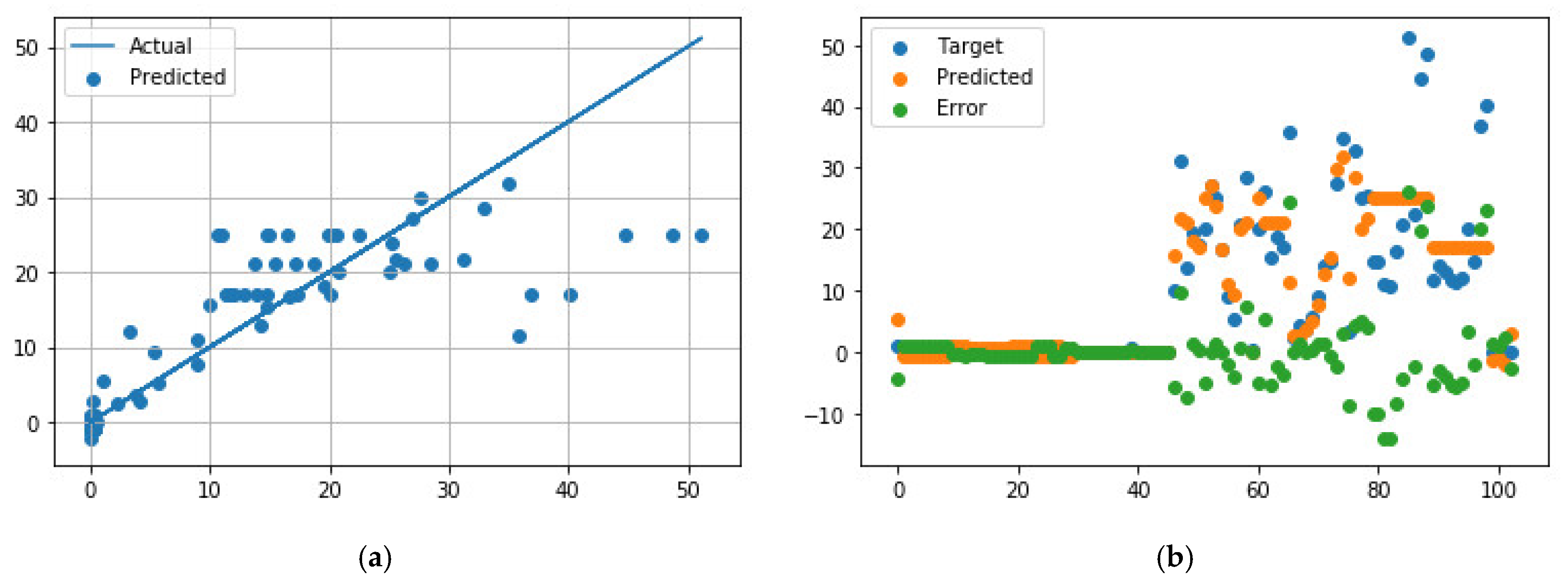
Figure 5.
Comparison of predicted and measured ER values for EB-PVD data points using the best NN model parameters. (a) Predicted values vs. actual values; (b) Distribution of actual values, predicted values, and errors.
Figure 5.
Comparison of predicted and measured ER values for EB-PVD data points using the best NN model parameters. (a) Predicted values vs. actual values; (b) Distribution of actual values, predicted values, and errors.
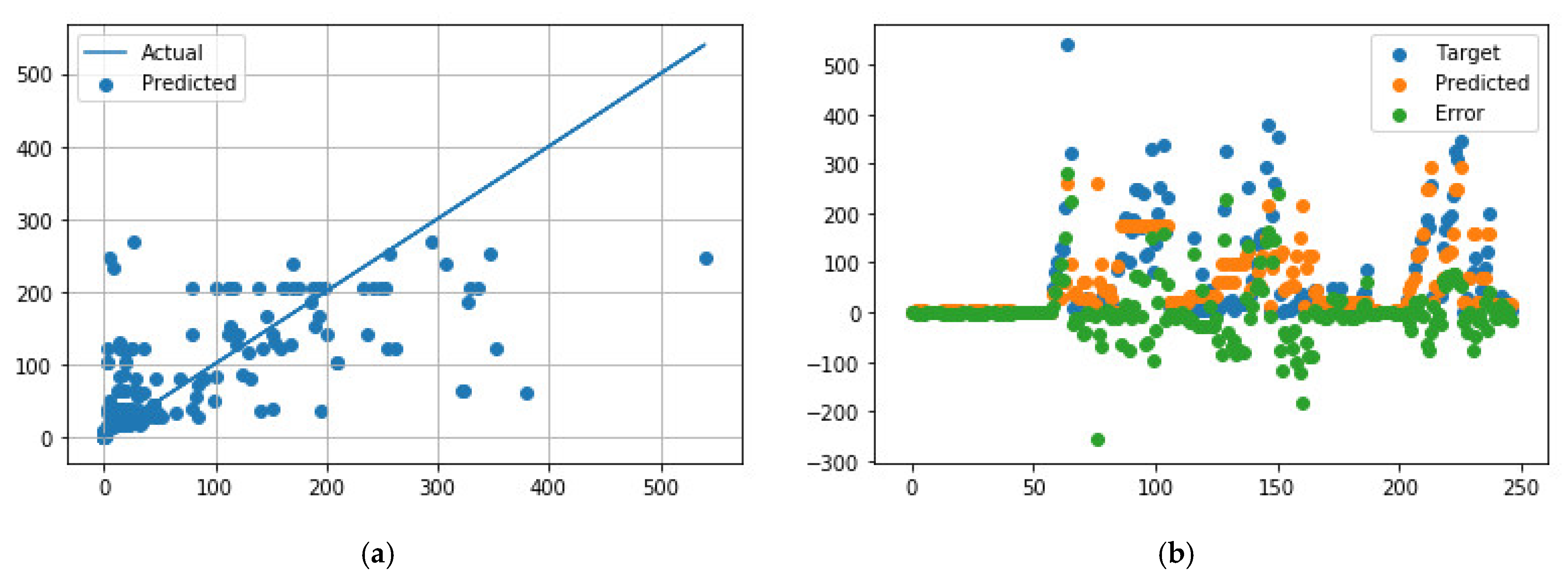
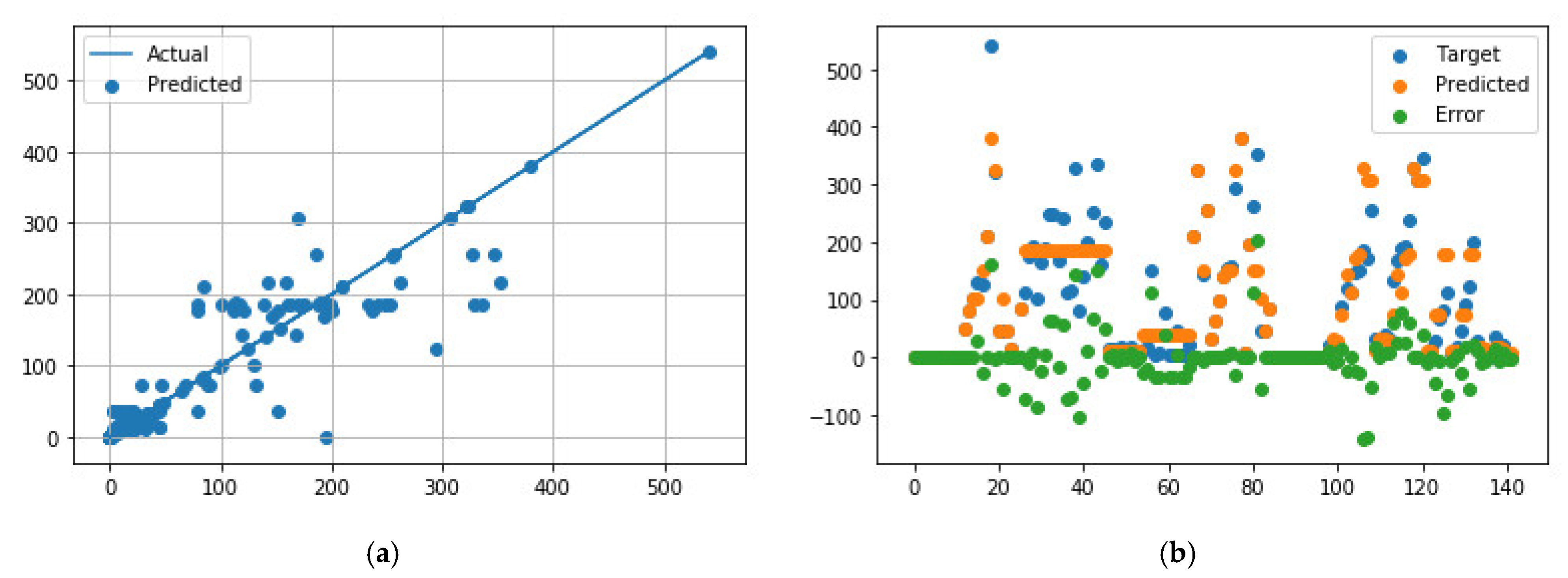
Figure 6.
Comparison of predicted and measured ER values for APS + EB-PVD data points using the best GB model parameters. (a) Predicted values vs. actual values; (b) Distribution of actual values, predicted values, and errors.
Figure 6.
Comparison of predicted and measured ER values for APS + EB-PVD data points using the best GB model parameters. (a) Predicted values vs. actual values; (b) Distribution of actual values, predicted values, and errors.
Figure 7.
Comparison of predicted and measured ER values for APS TBC data points using the best GB model parameters. (a) Predicted values vs. actual values; (b) Distribution of actual values, predicted values, and errors.
Figure 7.
Comparison of predicted and measured ER values for APS TBC data points using the best GB model parameters. (a) Predicted values vs. actual values; (b) Distribution of actual values, predicted values, and errors.
Figure 8.
Comparison of predicted and measured ER values for EB-PVD TBC data points using the best GB model parameters. (a) Predicted values vs. actual values; (b) Distribution of actual values, predicted values, and errors.
Figure 8.
Comparison of predicted and measured ER values for EB-PVD TBC data points using the best GB model parameters. (a) Predicted values vs. actual values; (b) Distribution of actual values, predicted values, and errors.
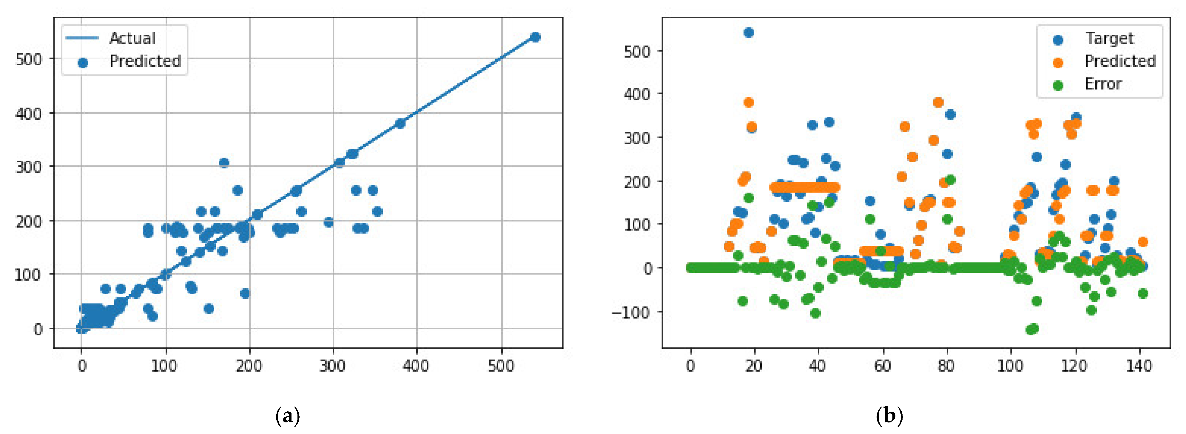
Figure 9.
Comparison of predicted and measured ER values for all TBC data points using the best TDR model parameters. (a) Predicted values vs. actual values; (b) Distribution of actual values, predicted values, and errors.
Figure 9.
Comparison of predicted and measured ER values for all TBC data points using the best TDR model parameters. (a) Predicted values vs. actual values; (b) Distribution of actual values, predicted values, and errors.
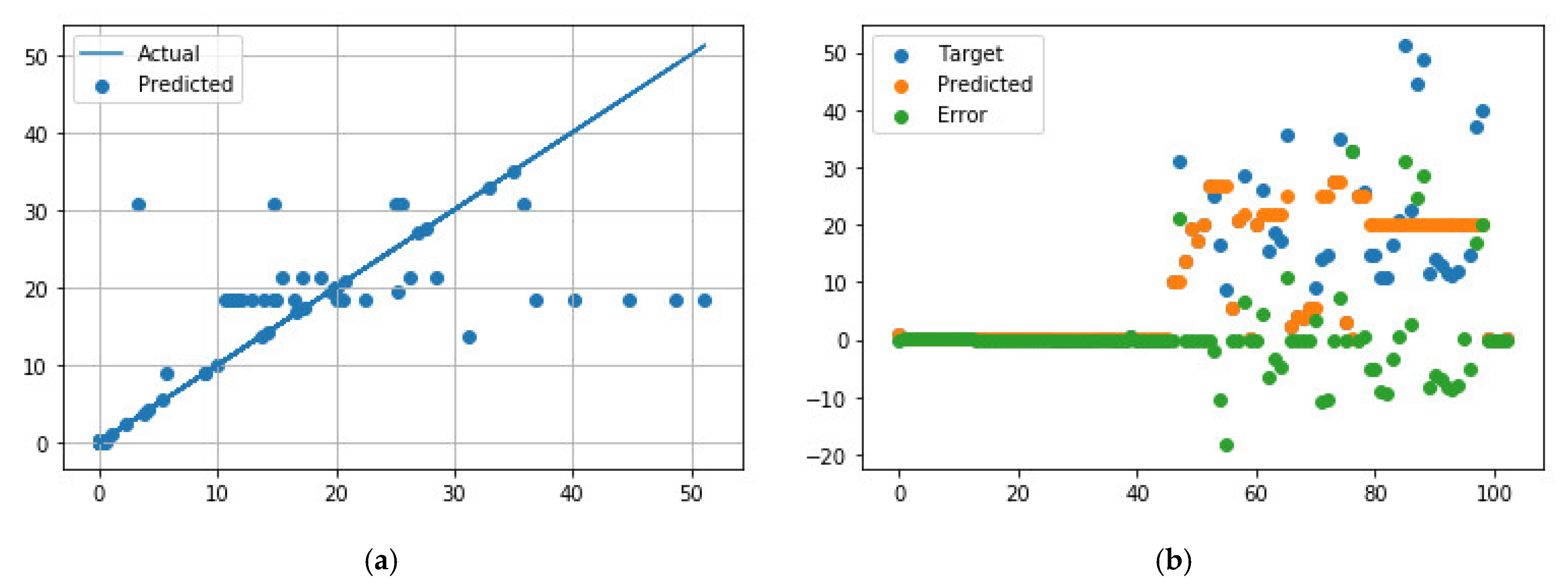
Figure 10.
Comparison of predicted and measured ER values for APS TBC data points using the best TDR model parameters. (a) Predicted values vs. actual values; (b) Distribution of actual values, predicted values, and errors.
Figure 10.
Comparison of predicted and measured ER values for APS TBC data points using the best TDR model parameters. (a) Predicted values vs. actual values; (b) Distribution of actual values, predicted values, and errors.
Figure 11.
Comparison of predicted and measured ER values for EB-PVD TBC data points using the best TDR model parameters. (a) Predicted values vs. actual values; (b) Distribution of actual values, predicted values, and errors.
Figure 11.
Comparison of predicted and measured ER values for EB-PVD TBC data points using the best TDR model parameters. (a) Predicted values vs. actual values; (b) Distribution of actual values, predicted values, and errors.
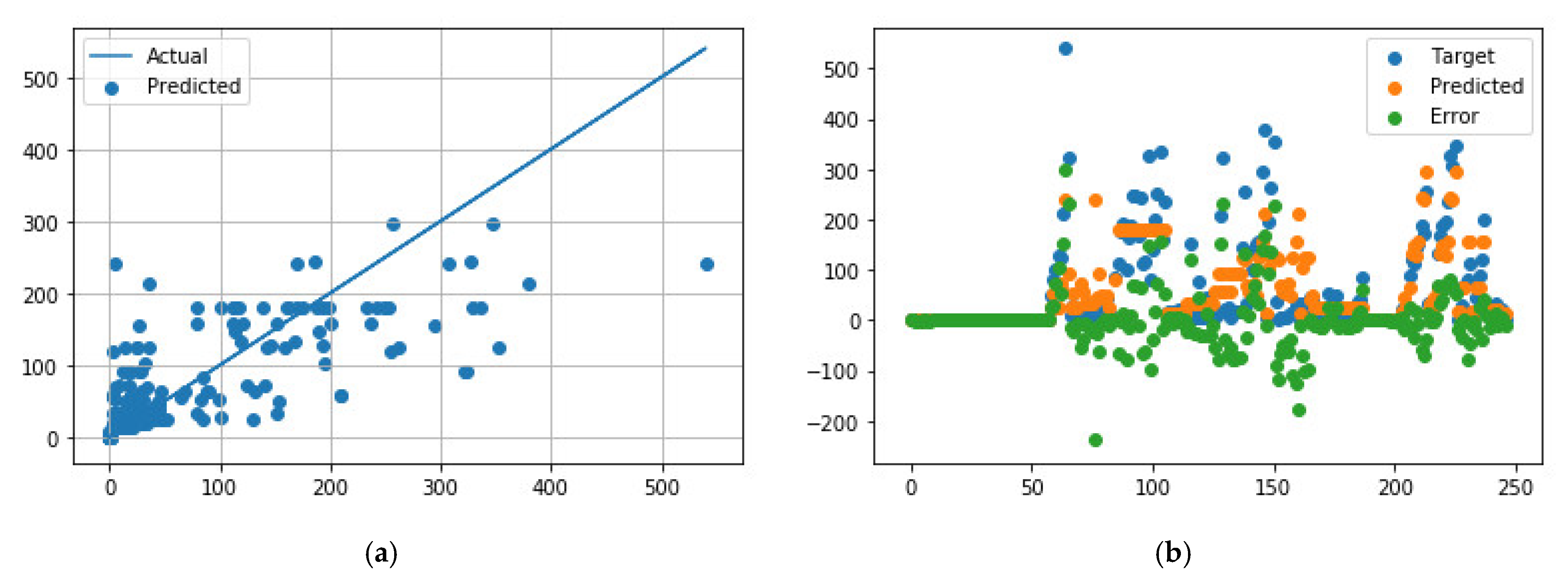
Figure 12.
Comparison of predicted and measured ER values for all TBC data points using the best RFR model parameters. (a) Predicted values vs. actual values; (b) Distribution of actual values, predicted values, and errors.
Figure 12.
Comparison of predicted and measured ER values for all TBC data points using the best RFR model parameters. (a) Predicted values vs. actual values; (b) Distribution of actual values, predicted values, and errors.
Figure 13.
Comparison of predicted and measured ER values for APS TBC data points using the best RFR model parameters. (a) Predicted values vs. actual values; (b) Distribution of actual values, predicted values, and errors.
Figure 13.
Comparison of predicted and measured ER values for APS TBC data points using the best RFR model parameters. (a) Predicted values vs. actual values; (b) Distribution of actual values, predicted values, and errors.
Figure 14.
Comparison of predicted and measured ER values for APS TBC data points using the best RFR model parameters. (a) Predicted values vs. actual values; (b) Distribution of actual values, predicted values, and errors.
Figure 14.
Comparison of predicted and measured ER values for APS TBC data points using the best RFR model parameters. (a) Predicted values vs. actual values; (b) Distribution of actual values, predicted values, and errors.
Figure 15.
The process to obtain the thermal conductivity of a coating [
41].
Figure 15.
The process to obtain the thermal conductivity of a coating [
41].
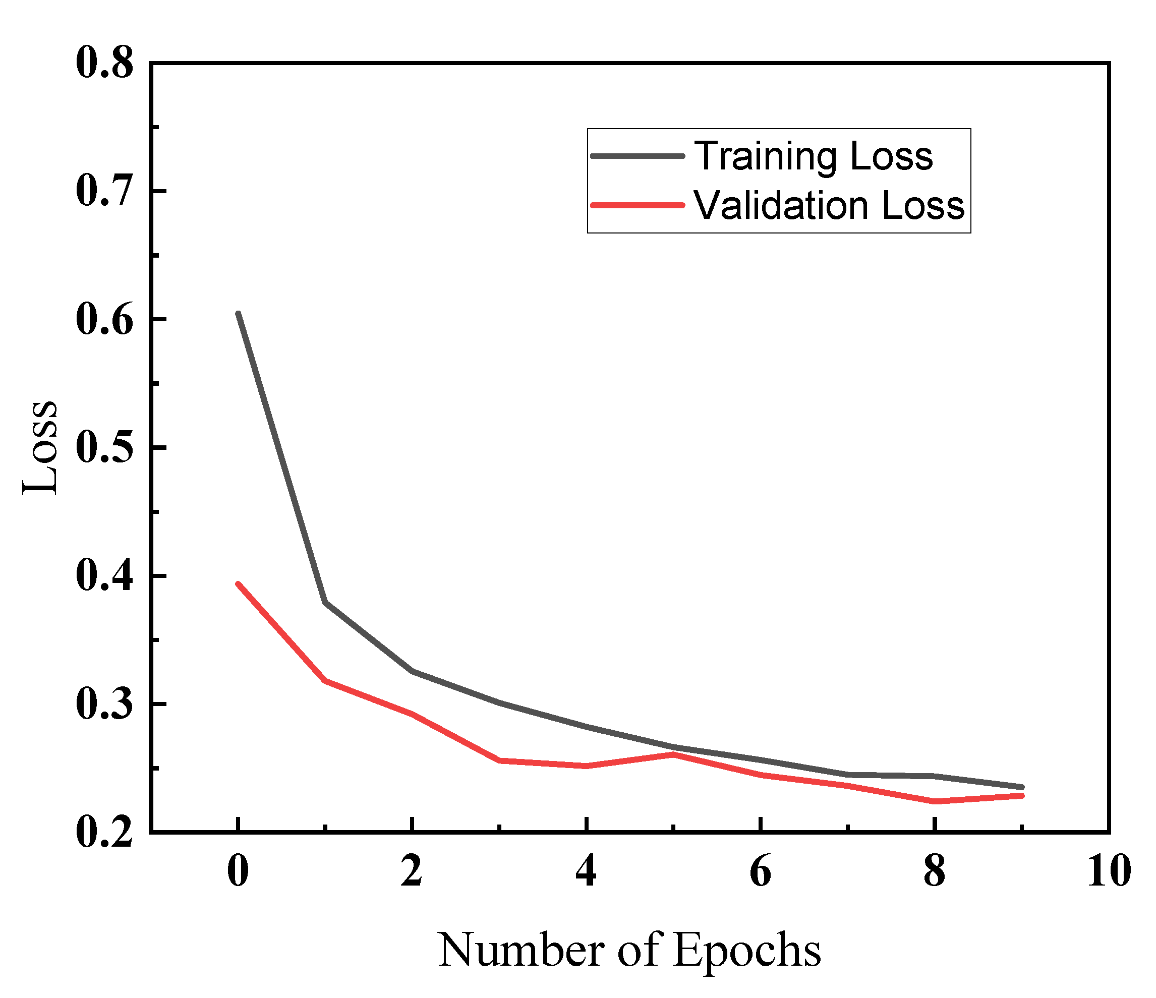
Figure 16.
Training and validation loss (Y axis) for different epochs (X axis) using the CNNs model for a fashion preliminary case.
Figure 16.
Training and validation loss (Y axis) for different epochs (X axis) using the CNNs model for a fashion preliminary case.
Table 1.
Summarised experimental research studies on erosion rates of TBCs.
Table 1.
Summarised experimental research studies on erosion rates of TBCs.
| Ref. No. | Year | Author | Material | Research Topic |
|---|
| [9] | 1998 | Davis | 6.6%–20% Y2O3-ZrO2 and of four and eight layers of Al2O3-ZrO2 | Erosion rate vs. TBC Thickness, TBC Surface roughness, Impact particle size, Particle velocity, Impingement angle, Test temperature (Room temp) |
| [10] | 1998 | Bruce | 7% Y2O3-ZrO2 | Erosion rate vs. TBC Thickness, Impact particle size, Particle velocity, Impingement angle, Test temperature;
Equivalent equations |
| [11] | 1998 | Nicholls | APS and EB-PVD 7% Y2O3-ZrO2 | Erosion rate vs. TBC Thickness, TBC Surface roughness, Impact particle size, Particle velocity, Impingement angle, Test temperature, and Erodent types |
| [12] | 1999 | Eaton | APS 7.5% Y2O3-ZrO2 | Erosion rate vs. TBC Thickness, Impact particle size, Particle velocity, Impingement angle, Test temperature
Function of erosion rate as velocity |
| [5] | 1999 | Janos | APS 7.5% Y2O3-ZrO2 | Erosion rate vs. TBC Thickness, Hardness, Impact particle size, Particle velocity, Impingement angle, Test temperature, Erodent types, Porosity, Ageing temp and time.
Function of erosion rate as micro-hardness |
| [13] | 1999 | Nicholls | EB-PVD 8% Y2O3-ZrO2 | Erosion rate vs. Impact particle size, Particle velocity, Impingement angle, Test temperature, Erodent types |
| [14] | 2003 | Nicholls | EB-PVD 8% Y2O3-ZrO2 | Erosion rate vs. Impact particle size, Particle velocity, Impingement angle, Test temperature, Erodent types |
| [15] | 2009 | Wellman | APS and EB-PVD 7% Y2O3-ZrO2 | Erosion rate vs. Impact particle size, Particle velocity, Impingement angle, Test temperature, Erodent types |
| [16] | 2011 | Cernuschi | APS and EB-PVD 7.5~8% Y2O3-ZrO2 | Erosion rate vs. TBC Thickness, hardness, Impact particle size, Particle velocity, Impingement angle, Test temperature, Erodent types, Porosity, Ageing temp and time.; Function of erosion rate as micro-hardness |
| [17] | 2018 | Shin and Hamed | APS 7% Y2O3-ZrO2 | Erosion rate vs. TBC Thickness, hardness, Impact particle size, Particle velocity, Impingement angle, Test temperature, Erodent types, Porosity, Ageing temp and time.; Function of erosion rate as micro-hardness |
Table 2.
Summarised data of EB-PVD YSZ TBC.
Table 2.
Summarised data of EB-PVD YSZ TBC.
| Ref. No. | Year | Author | APS Sample No. | EB-PBD Sample No. | Total |
|---|
| [9] | 1998 | Davis | 12 | 1 | 13 |
| [10] | 1998 | Bruce | 0 | 45 | 45 |
| [11] | 1998 | Nicholls | 14 | 14 | 28 |
| [12] | 1999 | Eaton | 28 | 0 | 28 |
| [5] | 1999 | Janos | 12 | 0 | 12 |
| [13] | 1999 | Nicholls | 10 | 0 | 10 |
| [14] | 1999 | Nicholls | 16 | 14 | 30 |
| [15] | 2009 | Wellman | 1 | 20 | 21 |
| [16] | 2011 | Cernuschi | 5 | 9 | 14 |
| [17] | 2017 | Shi | 44 | 0 | 44 |
| total | - | - | 142 | 103 | 245 |
Table 3.
Summarised experimental research on erosion rates of TBCs.
Table 3.
Summarised experimental research on erosion rates of TBCs.
| Variables | Unit | Description | Function |
|---|
| Material | W/(m∙K) | wt.% of Y2O3 | Inputs |
| Impact Angle | Degree | Impact angle of particles |
| Impact Velocity | m/s | Impact velocity of particles |
| Particle Size | micron | Diameter of erodent particles |
| TestTemp | °C | Temperature during measurement |
| Target ER | g/kg | Erosion rate of TBC | Output |
Table 4.
Correlation coefficients for all TBC data.
Table 4.
Correlation coefficients for all TBC data.
| Parameters | Material | Impact Angle | Impact V | Particle Size | Test Temp | Erosion Rate |
|---|
| Material | 1 | −0.03194 | −0.09196 | −0.04592 | −0.26285 | −0.02612 |
| Impact Angle | −0.03194 | 1 | −0.42818 | 0.356322 | −0.04395 | −0.13179 |
| Impact V | −0.09196 | −0.42818 | 1 | −0.48263 | 0.374805 | 0.54068 |
| Particle Size | −0.04592 | 0.356322 | −0.48263 | 1 | 0.186174 | −0.24137 |
| Test Temp | −0.26285 | −0.04395 | 0.374805 | 0.186174 | 1 | 0.049198 |
| Errosion Rate | −0.02612 | −0.13179 | 0.54068 | −0.24137 | 0.049198 | 1 |
Table 5.
Correlation coefficients for APS TBC data.
Table 5.
Correlation coefficients for APS TBC data.
| Title | Material | Impact Angle | Impact V | Particle Size | Test Temp | Errosion Rate |
|---|
| Material | 1 | 0.142241 | −0.18374 | 0.332938 | −0.24079 | −0.08089 |
| Impact Angle | 0.142241 | 1 | −0.32357 | 0.310126 | −0.2549 | 0.229697 |
| Impact V | −0.18374 | −0.32357 | 1 | −0.47894 | 0.640075 | 0.495648 |
| Particle Size | 0.332938 | 0.310126 | −0.47894 | 1 | −0.30445 | −0.21112 |
| Test Temp | −0.24079 | −0.2549 | 0.640075 | −0.30445 | 1 | 0.145308 |
| Errosion Rate | −0.08089 | 0.229697 | 0.495648 | −0.21112 | 0.145308 | 1 |
Table 6.
Correlation coefficients for EB-PVD TBC data.
Table 6.
Correlation coefficients for EB-PVD TBC data.
| Parameters | Material | Impact Angle | Impact V | Particle Size | Test Temp | Errosion Rate |
|---|
| Material | 1 | −0.30787 | 0.034516 | −0.15291 | −0.30402 | 0.061988 |
| Impact Angle | −0.30787 | 1 | −0.12055 | 0.205277 | 0.257427 | 0.004347 |
| Impact V | 0.034516 | −0.12055 | 1 | −0.70291 | 0.013128 | 0.242658 |
| Particle Size | −0.15291 | 0.205277 | −0.70291 | 1 | 0.358358 | −0.30279 |
| Test Temp | −0.30402 | 0.257427 | 0.013128 | 0.358358 | 1 | −0.59386 |
| Errosion Rate | 0.061988 | 0.004347 | 0.242658 | −0.30279 | −0.59386 | 1 |
Table 7.
Quick test results for all TBC data.
Table 7.
Quick test results for all TBC data.
| Features | RAlg | MSE | MAE | R2 | AdjR2 | PRESS | BIC | GCV |
|---|
| 5 | LR | 5599.136 | 51.0778 | 0.3463 | 0.3327 | 52.9465 | 2164.757 | 1,452,706 |
| 5 | GB | 4143.612 | 41.9211 | 0.5162 | 0.5062 | 43.4084 | 2090.399 | 1,075,068 |
| 5 | RF | 3403.455 | 31.0987 | 0.6026 | 0.5944 | 32.1065 | 2041.795 | 883,032.7 |
| 5 | DT | 3184.008 | 30.2029 | 0.6282 | 0.6205 | 31.187 | 2025.333 | 826,096.7 |
| 5 | KNN | 4591.058 | 40.6564 | 0.464 | 0.4528 | 42.1395 | 2115.727 | 1,191,158 |
| 5 | RIDGE | 6333.306 | 55.1329 | 0.2605 | 0.2452 | 57.0639 | 2195.19 | 1,643,188 |
| 5 | LASSO | 7581.492 | 63.9384 | 0.1148 | 0.0964 | 66.0237 | 2239.622 | 1,967,032 |
| 5 | AB | 4197.602 | 41.752 | 0.5099 | 0.4997 | 43.1949 | 2093.597 | 1,089,075 |
| 5 | SV | 7451.062 | 42.7329 | 0.13 | 0.112 | 44.313 | 2235.336 | 1,933,192 |
Table 8.
Quick test results for APS TBC data.
Table 8.
Quick test results for APS TBC data.
| Features | RAlg | MSE | MAE | R2 | AdjR2 | PRESS | BIC | GCV |
|---|
| 5 | LR | 6315.652 | 60.1596 | 0.4588 | 0.439 | 62.7441 | 1281.14 | 983,977.6 |
| 5 | GB | 3552.395 | 45.6964 | 0.6956 | 0.6845 | 47.4223 | 1198.856 | 553,462.5 |
| 5 | RF | 1454.941 | 24.0177 | 0.8753 | 0.8708 | 24.9086 | 1071.206 | 226,679.5 |
| 5 | DT | 1115.415 | 17.1148 | 0.9044 | 0.9009 | 17.7995 | 1033.206 | 173,781.5 |
| 5 | KNN | 5812.361 | 55.3393 | 0.5019 | 0.4837 | 57.6708 | 1269.264 | 905,564.9 |
| 5 | RIDGE | 7960.008 | 68.9798 | 0.3178 | 0.293 | 71.7985 | 1314.23 | 1,240,168 |
| 5 | LASSO | 9680.04 | 78.8275 | 0.1704 | 0.1402 | 82.1582 | 1342.206 | 1,508,149 |
| 5 | AB | 3142.537 | 46.3897 | 0.7307 | 0.7209 | 48.2247 | 1181.325 | 489,606.7 |
| 5 | SV | 7627.288 | 58.6225 | 0.3464 | 0.3225 | 60.8968 | 1308.124 | 1,188,330 |
Table 9.
Quick test results for EB-PBD TBC data.
Table 9.
Quick test results for EB-PBD TBC data.
| Features | RAlg | MSE | MAE | R2 | AdjR2 | PRESS | BIC | GCV |
|---|
| 5 | LR | 84.191 | 6.5402 | 0.4797 | 0.4526 | 7.5648 | 479.9248 | 9694.465 |
| 5 | GB | 58.5397 | 5.0387 | 0.6382 | 0.6194 | 5.6239 | 442.8598 | 6740.761 |
| 5 | RF | 42.2348 | 3.4883 | 0.739 | 0.7254 | 3.6952 | 409.5608 | 4863.272 |
| 5 | DT | 34.6876 | 2.4219 | 0.7856 | 0.7745 | 2.5633 | 389.4808 | 3994.224 |
| 5 | KNN | 70.8368 | 5.2107 | 0.5622 | 0.5394 | 5.5297 | 462.3084 | 8156.746 |
| 5 | RIDGE | 105.8371 | 7.8759 | 0.3459 | 0.3119 | 9.432 | 503.2637 | 12,186.97 |
| 5 | LASSO | 161.8108 | 10.4959 | 0 | −0.0521 | 12.5985 | 546.5655 | 18,632.27 |
| 5 | AB | 55.6216 | 4.5628 | 0.6563 | 0.6384 | 4.8273 | 437.6442 | 6404.744 |
| 5 | SV | 68.6382 | 4.0034 | 0.5758 | 0.5537 | 4.2498 | 459.0924 | 7903.579 |
Table 10.
Performances of ER prediction using the NN approach for APS + EB-PVD TBC data.
Table 10.
Performances of ER prediction using the NN approach for APS + EB-PVD TBC data.
| Hyper-Parameters | Train | Test | All |
|---|
| Number of Nodes | Repeat | R2 | MSE | MAXE | R2 | MSE | MAXE | R2 | MSE | MAXE |
|---|
| 10 | 100 | 0.4740 | 4570.4 | 327.79 | 0.3329 | 6031 | 261.04 | 0.4463 | 4791 | 348.23 |
| 20 | 100 | 0.4636 | 4649.6 | 334.95 | 0.3240 | 6786.9 | 269.54 | 0.4306 | 4972.3 | 357.01 |
| 30 | 100 | 0.5627 | 3735.4 | 290.14 | 0.2789 | 9322 | 322.22 | 0.4847 | 4579.1 | 372.07 |
| 40 | 100 | 0.5310 | 4013 | 306.53 | 0.3377 | 6865.9 | 289.63 | 0.4871 | 4443.8 | 355.04 |
| 50 | 100 | 0.5436 | 3891.7 | 298.03 | 0.3211 | 8374.8 | 317.36 | 0.4838 | 4568.7 | 373.41 |
| 60 | 100 | 0.5371 | 3988.7 | 300.58 | 0.3021 | 7824.4 | 298.21 | 0.4767 | 4567.9 | 364.35 |
Table 11.
Performances of ER prediction using the NN approach for APS TBC data.
Table 11.
Performances of ER prediction using the NN approach for APS TBC data.
| Hyper-Parameters | Train | Test | All |
|---|
| Number of Nodes | Repeat | R2 | MSE | MAXE | R2 | MSE | MAXE | R2 | MSE | MAXE |
|---|
| 5 | 100 | 0.8340 | 1958.3 | 159.21 | 0.6473 | 4388 | 178.58 | 0.8034 | 2317.6 | 192.14 |
| 10 | 100 | 0.8540 | 1732.2 | 155.81 | 0.6524 | 4196.8 | 181.08 | 0.8219 | 2096.7 | 190.42 |
| 15 | 100 | 0.8419 | 1851.3 | 157.04 | 0.6554 | 4394 | 180.7 | 0.8108 | 2227.4 | 190.86 |
| 20 | 100 | 0.8687 | 1535.6 | 149.59 | 0.6991 | 3946.7 | 170.84 | 0.8400 | 1892.2 | 184.01 |
| 25 | 100 | 0.8510 | 1750.6 | 158.41 | 0.6701 | 4022.3 | 171.5 | 0.8227 | 2086.5 | 187.81 |
| 30 | 100 | 0.8428 | 1849.8 | 158.17 | 0.6625 | 4391.2 | 178.8 | 0.8116 | 2225.6 | 194.69 |
| 35 | 100 | 0.8549 | 1702.6 | 152.25 | 0.6816 | 4211.6 | 172.59 | 0.8245 | 2073.6 | 188.45 |
| 40 | 100 | 0.8459 | 1843.8 | 157.39 | 0.6146 | 4737.9 | 191.73 | 0.8078 | 2271.8 | 204.34 |
Table 12.
Performances of ER prediction using the NN approach for EB-PVD TBC data.
Table 12.
Performances of ER prediction using the NN approach for EB-PVD TBC data.
| Hyper-Parameters | Train | Test | All |
|---|
| Number of Nodes | Repeat | R2 | MSE | MAXE | R2 | MSE | MAXE | R2 | MSE | MAXE |
|---|
| 5 | 100 | 0.7106 | 46.684 | 27.339 | 0.6039 | 83.216 | 22.887 | 0.6802 | 52.004 | 28.305 |
| 10 | 100 | 0.7147 | 46.416 | 27.294 | 0.5868 | 81.478 | 22.99 | 0.6827 | 51.522 | 28.253 |
| 15 | 100 | 0.7118 | 46.457 | 27.529 | 0.5893 | 86.439 | 23.182 | 0.6786 | 52.28 | 28.627 |
| 20 | 100 | 0.7027 | 47.918 | 27.771 | 0.5909 | 79.554 | 22.685 | 0.6765 | 52.525 | 28.602 |
| 25 | 100 | 0.7025 | 48.234 | 27.534 | 0.6146 | 75.217 | 21.724 | 0.6782 | 52.164 | 28.384 |
| 30 | 100 | 0.6983 | 48.857 | 27.83 | 0.6253 | 73.212 | 21.032 | 0.6769 | 52.403 | 28.321 |
| 35 | 100 | 0.6983 | 48.895 | 27.917 | 0.6162 | 72.445 | 21.073 | 0.6767 | 52.324 | 28.502 |
| 40 | 100 | 0.6938 | 50.019 | 27.534 | 0.6465 | 70.822 | 20.763 | 0.6729 | 53.049 | 28.303 |
Table 13.
Values of parameters of GBR.
Table 13.
Values of parameters of GBR.
| Parameters | Description | Options or Values | Default Values |
|---|
| loss | Loss function to be optimised | String, ‘ls’, ‘lad’, ‘huber’, ‘quantile’ | ls |
| learning_rate | Learning rate shrinks the contribution of each tree | float, optional | 0.055 |
| n_estimators | The number of boosting stages to perform | int | 400 |
| subsample | The fraction of samples to be used for fitting the individual base learners | float | 1.0 |
| min_samples_split | The minimum number of samples required to split an internal node | int, float, optional | 4 |
| min_weight_fraction_leaf | The minimum weighted fraction of the sum total of weights (of all the input samples) required to be at a leaf node. | float, optional | 0 |
| max_depth | Maximum depth of the individual regression estimators | integer, optional | 4 |
| min_impurity_decrease | A node will be split if this split induces a decrease of the impurity greater than or equal to this value | float, optional | 0 |
| min_impurity_split | Threshold for early stopping in tree growth | float | 1 × 10⁻⁷ |
| validation_fraction | The proportion of training data to set aside as the validation set for early stopping | float | 0.1 |
| tot | Tolerance for the early stopping | float, optional | 1 × 10⁻⁴ |
| ccp_alpha | Complexity parameter used for minimal cost-complexity pruning | non-negative float, optional | 0.0 |
Table 14.
Performances of ER prediction using the GBR approach for all TBC data.
Table 14.
Performances of ER prediction using the GBR approach for all TBC data.
| Hyper-Parameters | Train | Test | All |
|---|
| N of Est. | Max Dep. | Min Sample Split | Learning Rate | Repeat | R2 | MSE | MAXE | R2 | MSE | MAXE | R2 | MSE | MAXE |
|---|
| 500 | 4 | 6 | 0.01 | 10 | 0.6499 | 2906.54 | 265.85 | 0.2498 | 7390.64 | 370.12 | 0.5547 | 3814.25 | 378.42 |
| 500 | 4 | 2 | 0.01 | 10 | 0.6509 | 2898.25 | 263.29 | 0.2359 | 7531.86 | 377.20 | 0.5521 | 3836.23 | 383.77 |
| 100 | 4 | 6 | 0.01 | 10 | 0.5136 | 4029.38 | 322.12 | 0.2876 | 7036.15 | 347.88 | 0.4585 | 4638.04 | 397.26 |
| 1000 | 4 | 6 | 0.01 | 10 | 0.6531 | 2880.90 | 258.56 | 0.2116 | 7760.85 | 380.09 | 0.5483 | 3868.74 | 384.41 |
| 500 | 4 | 6 | 0.1 | 10 | 0.6533 | 2878.55 | 256.78 | 0.1973 | 7879.10 | 380.96 | 0.5457 | 3890.80 | 384.03 |
| 500 | 2 | 6 | 0.01 | 10 | 0.5846 | 3447.75 | 314.67 | 0.3552 | 6359.93 | 333.17 | 0.5286 | 4037.26 | 386.36 |
Table 15.
Performances of ER prediction using the GBR approach for APS TBC data.
Table 15.
Performances of ER prediction using the GBR approach for APS TBC data.
| Hyper-Parameters | Train | Test | All |
|---|
| N of Est. | Max Dep. | Min Sample Split | Learning Rate | Repeat | R2 | MSE | MAXE | R2 | MSE | MAXE | R2 | MSE | MAXE |
|---|
| 10 | 4 | 6 | 0.2 | 10 | 0.8484 | 1785.11 | 157.87 | 0.6208 | 3959.35 | 170.14 | 0.8093 | 2229.15 | 179.94 |
| 500 | 4 | 6 | 0.2 | 10 | 0.8815 | 1395.88 | 146.29 | 0.6595 | 3447.56 | 161.86 | 0.8447 | 1814.88 | 163.96 |
| 500 | 4 | 6 | 0.01 | 10 | 0.8792 | 1422.32 | 147.88 | 0.6679 | 3403.43 | 159.31 | 0.8437 | 1826.91 | 166.05 |
| 500 | 4 | 2 | 0.2 | 10 | 0.8815 | 1395.88 | 146.29 | 0.6548 | 3534.03 | 167.08 | 0.8432 | 1832.54 | 170.08 |
| 500 | 6 | 6 | 0.2 | 10 | 0.8815 | 1395.88 | 146.29 | 0.6229 | 3853.18 | 175.80 | 0.8376 | 1897.72 | 176.89 |
| 500 | 2 | 6 | 0.2 | 10 | 0.8815 | 1395.90 | 146.29 | 0.6632 | 3518.42 | 168.74 | 0.8435 | 1829.37 | 171.89 |
Table 16.
Performances of ER prediction using the GBR approach for EB-PVD TBC data.
Table 16.
Performances of ER prediction using the GBR approach for EB-PVD TBC data.
| Hyper-Parameters | Train | Test | All |
|---|
| N of Est. | Max Dep. | Min Sample Split | Learning Rate | Repeat | R2 | MSE | MAXE | R2 | MSE | MAXE | R2 | MSE | MAXE |
|---|
| 500 | 4 | 2 | 0.01 | 10 | 0.7705 | 34.98 | 29.52 | 0.4736 | 100.51 | 27.88 | 0.7000 | 48.34 | 30.83 |
| 500 | 6 | 2 | 0.01 | 10 | 0.7709 | 34.91 | 29.51 | 0.4707 | 103.48 | 28.04 | 0.6966 | 48.89 | 31.00 |
| 1000 | 4 | 2 | 0.01 | 10 | 0.7710 | 34.90 | 29.44 | 0.4709 | 100.89 | 27.82 | 0.6999 | 48.35 | 30.75 |
| 500 | 4 | 6 | 0.01 | 10 | 0.7702 | 35.02 | 29.55 | 0.4681 | 101.86 | 27.87 | 0.6981 | 48.65 | 30.81 |
| 500 | 4 | 6 | 0.1 | 10 | 0.7710 | 34.90 | 29.43 | 0.4652 | 102.33 | 27.72 | 0.6981 | 48.65 | 30.73 |
| 500 | 2 | 6 | 0.1 | 10 | 0.7420 | 39.30 | 30.62 | 0.4846 | 100.19 | 27.25 | 0.6791 | 51.72 | 31.12 |
Table 17.
Hyper-parameters of DTR.
Table 17.
Hyper-parameters of DTR.
| Parameters | Description | Options or Values | Default Values |
|---|
| criterion | The function to measure the quality of a split. | “mse”, “friedman_mse”, “mae” | ”mse” |
| Splitter | The strategy used to choose the split at each node. | “best”, “random” | ”best” |
| max_depth | The maximum depth of the tree. If none, then nodes are expanded until all leaves are pure or until all leaves contain less than min_samples_split samples. | integer, optional | None |
| min_samples_split | The minimum number of samples required to split an internal node. | int, float, optional | 2 |
| min_samples_leaf | The minimum number of samples required to be at a leaf node. | int, float, optional | 1 |
| min_weight_fraction_leaf | The minimum weighted fraction of the sum total of weights (of all the input samples) required to be at a leaf node. | float, optional | 0 |
| max_depth | Maximum depth of the individual regression estimators. | integer, optional | None |
| min_impurity_decrease | A node will be split if this split induces a decrease of the impurity greater than or equal to this value. | float, optional | 0 |
| min_impurity_split | Threshold for early stopping in tree growth. | float | 0 |
| random_state | Define the random number generator. | int, RandomState instance or none, optional | none |
| max_features | The number of features to consider when looking for the best split. | nt, float, string or none, optional | none |
| max_leaf_nodes | Grow trees with max_leaf_nodes in best-first fashion. | int or none, optional | none |
| tot | Tolerance for the early stopping. | float, optional | 1 × 10⁻⁴ |
| ccp_alpha | Complexity parameter used for Minimal Cost-Complexity Pruning. | non-negative float, optional | 0.0 |
Table 18.
Performances of ER prediction using the DTR approach for all TBC data.
Table 18.
Performances of ER prediction using the DTR approach for all TBC data.
| Hyper-Parameters | Train | Test | All |
|---|
| Min Sample Split | Min Samples Leaf | Min Weight Fraction Leaf | Min Impurity Decrease | CCP Alpha | R2 | MSE | MAXE | R2 | MSE | MAXE | R2 | MSE | MAXE |
|---|
| 2 (def) | 1 (def) | 0 (def) | 0 (def) | 0 (def) | 0.6533 | 2878.55 | 256.77 | 0.1407 | 8428.65 | 385.56 | 0.5327 | 4002.05 | 388.63 |
| 4 | 1 | 0 | 0 | 0 | 0.6510 | 2897.31 | 259.24 | 0.1711 | 8149.88 | 385.56 | 0.5376 | 3960.58 | 391.09 |
| 6 | 1 | 0 | 0 | 0 | 0.6402 | 2987.76 | 263.82 | 0.1745 | 8114.65 | 359.30 | 0.5300 | 4025.59 | 363.85 |
| 2 | 2 | 0 | 0 | 0 | 0.6311 | 3063.11 | 258.91 | 0.2243 | 7638.51 | 355.67 | 0.5342 | 3989.31 | 361.50 |
| 2 | 4 | 0 | 0 | 0 | 0.5753 | 3524.22 | 304.93 | 0.2163 | 7730.95 | 354.78 | 0.4891 | 4375.78 | 396.79 |
| 2 | 1 | 0.1 | 0 | 0 | 0.4510 | 4556.44 | 332.56 | 0.2946 | 6887.12 | 328.96 | 0.4129 | 5028.24 | 398.04 |
| 2 | 1 | 0 | 0.1 | 0 | 0.6533 | 2878.77 | 256.77 | 0.1351 | 8484.42 | 385.36 | 0.5314 | 4013.52 | 388.43 |
| 2 | 1 | 0 | 0.5 | 0 | 0.6531 | 2880.49 | 256.77 | 0.1313 | 8547.40 | 387.86 | 0.5297 | 4027.64 | 390.83 |
| 2 | 1 | 0 | 0 | 0.1 | 0.6533 | 2878.72 | 256.77 | 0.1413 | 8423.97 | 386.98 | 0.5328 | 4001.24 | 390.05 |
Table 19.
Performances of ER prediction using the DTR approach for APS TBC data.
Table 19.
Performances of ER prediction using the DTR approach for APS TBC data.
| Hyper-Parameters | Train | Test | All |
|---|
| Min Sample Split | Min Samples Leaf | Min Weight Fraction Leaf | Min Impurity Decrease | CCP Alpha | R2 | MSE | MAXE | R2 | MSE | MAXE | R2 | MSE | MAXE |
|---|
| 2 (def) | 1 (def) | 0 (def) | 0 (def) | 0 (def) | 0.8815 | 1395.88 | 146.29 | 0.6165 | 3846.94 | 178.08 | 0.8377 | 1896.45 | 178.55 |
| 4 | 1 | 0 | 0 | 0 | 0.8660 | 1570.00 | 146.00 | 0.6180 | 3840.00 | 175.00 | 0.8260 | 2040.00 | 176.00 |
| 6 | 1 | 0 | 0 | 0 | 0.8475 | 1801.79 | 148.55 | 0.5798 | 4204.34 | 181.52 | 0.8039 | 2292.45 | 184.13 |
| 2 | 2 | 0 | 0 | 0 | 0.8511 | 1752.10 | 146.45 | 0.6365 | 3637.31 | 170.61 | 0.8172 | 2137.11 | 173.96 |
| 2 | 4 | 0 | 0 | 0 | 0.7605 | 2825.72 | 180.90 | 0.5668 | 4430.75 | 184.93 | 0.7302 | 3153.51 | 204.16 |
| 2 | 1 | 0.1 | 0 | 0 | 0.5477 | 5354.25 | 302.01 | 0.3449 | 6983.93 | 211.96 | 0.5134 | 5687.07 | 311.16 |
| 2 | 1 | 0 | 0.1 | 0 | 0.8814 | 1395.96 | 146.29 | 0.6001 | 3983.24 | 180.32 | 0.8354 | 1924.35 | 180.85 |
| 2 | 1 | 0 | 0.5 | 0 | 0.8814 | 1396.75 | 146.29 | 0.6152 | 3846.68 | 177.98 | 0.8377 | 1897.09 | 178.52 |
| 2 | 1 | 0 | 0 | 0.1 | 0.8814 | 1395.96 | 146.29 | 0.6027 | 3973.13 | 172.68 | 0.8355 | 1922.29 | 174.17 |
Table 20.
Performances of ER prediction using the DTR approach for EB-PVD TBC data.
Table 20.
Performances of ER prediction using the DTR approach for EB-PVD TBC data.
| Hyper-Parameters | Train | Test | All |
|---|
| Min Sample Split | Min Samples Leaf | Min Weight Fraction Leaf | Min Impurity Decrease | CCP Alpha | R2 | MSE | MAXE | R2 | MSE | MAXE | R2 | MSE | MAXE |
|---|
| 2 (def) | 1 (def) | 0 (def) | 0 (def) | 0 (def) | 0.7710 | 34.90 | 29.43 | 0.4369 | 110.31 | 28.39 | 0.6880 | 50.27 | 31.07 |
| 4 | 1 | 0 | 0 | 0 | 0.7655 | 35.76 | 29.43 | 0.4118 | 113.58 | 29.02 | 0.6796 | 51.62 | 31.07 |
| 6 | 1 | 0 | 0 | 0 | 0.7512 | 37.85 | 29.43 | 0.4335 | 110.41 | 28.67 | 0.6733 | 52.64 | 31.07 |
| 2 | 2 | 0 | 0 | 0 | 0.7382 | 39.97 | 29.45 | 0.4635 | 104.07 | 28.30 | 0.6709 | 53.04 | 30.94 |
| 2 | 4 | 0 | 0 | 0 | 0.6951 | 46.55 | 29.35 | 0.4574 | 106.00 | 27.65 | 0.6359 | 58.67 | 30.89 |
| 2 | 1 | 0 | 0.5 | 0 | 0.7619 | 36.27 | 29.34 | 0.3928 | 118.04 | 28.51 | 0.6715 | 52.94 | 31.01 |
| 2 | 1 | 0 | 0 | 0.1 | 0.7695 | 35.13 | 29.41 | 0.4147 | 112.96 | 28.79 | 0.6835 | 51.00 | 31.07 |
Table 21.
Hyper-parameters of RFR.
Table 21.
Hyper-parameters of RFR.
| Parameters | Description | Options or Values | Default Values |
|---|
| n_estimators | The number of trees in the forest. | int | 0 |
| min_samples_split | The minimum number of samples required to split an internal node. | int, float | 2 |
| min_samples_leaf | The minimum number of samples required to be at a leaf node. | int, float | 1 |
| min_weight_fraction_leaf | The minimum weighted fraction of the sum total of weights (of all the input samples) required to be at a leaf node. | float, optional | 0 |
| max_depth | The maximum depth of the individual regression estimators. | integer, optional | None |
| min_impurity_decrease | A node will be split if this split induces a decrease of the impurity greater than or equal to this value. | float, optional | 0 |
| min_impurity_split | Threshold for early stopping in tree growth. | float | 0 |
| random_state | Define the random number generator. | int, RandomState instance or none, optional | none |
| max_samples | If bootstrap is true, the number of samples to draw from X to train each base estimator. | nt, float | none |
| max_leaf_nodes | Grow trees with max_leaf_nodes in best-first fashion. | int or none, optional | none |
| tot | Tolerance for the early stopping. | float, optional | 1 × 10⁻⁴ |
| ccp_alpha | Complexity parameter used for Minimal Cost-Complexity Pruning. | non-negative float, optional | 0.0 |
Table 22.
Performances of ER prediction using the RFR approach for all TBC data.
Table 22.
Performances of ER prediction using the RFR approach for all TBC data.
| Hyper-Parameters | Train | Test | All |
|---|
| N of Est. | Max Depth | Min Sample Split | Min Samples Leaf | CCP Alpha | R2 | MSE | MAXE | R2 | MSE | MAXE | R2 | MSE | MAXE |
|---|
| 10 | None | 2 | 1 | 0 | 0.6192 | 3160.65 | 285.89 | 0.2861 | 6938.43 | 322.91 | 0.5417 | 3925.38 | 351.92 |
| 100 | None | 2 | 1 | 0 | 0.6370 | 3013.81 | 281.62 | 0.2951 | 6921.69 | 342.92 | 0.5557 | 3804.88 | 369.92 |
| 200 | None | 2 | 1 | 0 | 0.6388 | 2998.72 | 274.95 | 0.2884 | 6981.54 | 345.30 | 0.5557 | 3804.96 | 366.62 |
| 500 | None | 2 | 1 | 0 | 0.6392 | 2995.33 | 271.86 | 0.2952 | 6913.27 | 344.76 | 0.5577 | 3788.44 | 361.61 |
| 500 | 4 | 2 | 1 | 0 | 0.5982 | 3330.92 | 273.38 | 0.3112 | 6760.09 | 342.04 | 0.5300 | 4025.08 | 357.77 |
| 500 | None | 4 | 1 | 0 | 0.6344 | 3035.32 | 281.25 | 0.3063 | 6801.32 | 339.83 | 0.5566 | 3797.67 | 365.95 |
| 500 | None | 2 | 2 | 0 | 0.6173 | 3176.67 | 296.32 | 0.3232 | 6643.01 | 332.11 | 0.5472 | 3878.35 | 374.16 |
| 500 | None | 2 | 1 | 0.1 | 0.6393 | 2995.18 | 270.86 | 0.2904 | 6975.11 | 345.43 | 0.5562 | 3800.83 | 362.98 |
Table 23.
Performances of ER prediction using the RFR approach for APS TBC data.
Table 23.
Performances of ER prediction using the RFR approach for APS TBC data.
| Hyper-Parameters | Train | Test | All |
|---|
| N of Est. | Max Depth | Min Sample Split | Min Samples Leaf | CCP Alpha | R2 | MSE | MAXE | R2 | MSE | MAXE | R2 | MSE | MAXE |
|---|
| 10 | None | 2 | 1 | 0 | 0.8392 | 1895.39 | 161.97 | 0.6250 | 3866.68 | 161.25 | 0.8034 | 2297.98 | 179.14 |
| 10 | 4 | 2 | 1 | 0 | 0.7973 | 2388.49 | 158.98 | 0.5914 | 4259.93 | 164.94 | 0.7629 | 2770.68 | 180.05 |
| 100 | None | 2 | 1 | 0 | 0.8540 | 1721.07 | 145.01 | 0.6503 | 3637.27 | 162.41 | 0.8193 | 2112.40 | 172.57 |
| 200 | None | 2 | 1 | 0 | 0.8544 | 1715.10 | 146.13 | 0.6582 | 3583.94 | 163.83 | 0.8206 | 2096.76 | 173.64 |
| 500 | None | 2 | 1 | 0 | 0.8543 | 1717.74 | 146.05 | 0.6598 | 3558.09 | 159.80 | 0.8209 | 2093.59 | 170.63 |
| 500 | None | 4 | 1 | 0 | 0.8406 | 1881.33 | 155.41 | 0.6531 | 3621.78 | 161.01 | 0.8086 | 2236.77 | 177.53 |
| 500 | None | 2 | 2 | 0 | 0.8167 | 2162.93 | 186.94 | 0.6549 | 3664.26 | 163.54 | 0.7887 | 2469.54 | 205.84 |
| 500 | None | 2 | 1 | 0.1 | 0.8548 | 1710.61 | 146.14 | 0.6548 | 3617.42 | 160.30 | 0.8203 | 2100.03 | 171.64 |
Table 24.
Performances of ER prediction using the RFR approach for EB-PVD TBC data.
Table 24.
Performances of ER prediction using the RFR approach for EB-PVD TBC data.
| Hyper-Parameters | Train | Test | All |
|---|
| N of Est. | Max Depth | Min Sample Split | Min Samples Leaf | CCP Alpha | R2 | MSE | MAXE | R2 | MSE | MAXE | R2 | MSE | MAXE |
|---|
| 10 | None | 2 | 1 | 0 | 0.7369 | 39.98 | 29.59 | 0.5000 | 99.22 | 26.31 | 0.6770 | 52.05 | 30.17 |
| 100 | None | 2 | 1 | 0 | 0.7468 | 38.54 | 29.60 | 0.5189 | 95.16 | 26.37 | 0.6892 | 50.09 | 30.45 |
| 200 | None | 2 | 1 | 0 | 0.7465 | 38.58 | 29.42 | 0.5171 | 94.80 | 26.49 | 0.6894 | 50.04 | 30.18 |
| 500 | None | 2 | 1 | 0 | 0.7473 | 38.47 | 29.46 | 0.5175 | 94.83 | 26.40 | 0.6900 | 49.96 | 30.25 |
| 500 | 4 | 2 | 1 | 0 | 0.7274 | 41.47 | 29.41 | 0.5244 | 93.29 | 26.37 | 0.6771 | 52.04 | 30.18 |
| 500 | None | 4 | 1 | 0 | 0.7405 | 39.49 | 29.39 | 0.5196 | 94.17 | 26.27 | 0.6857 | 50.64 | 30.18 |
| 500 | None | 2 | 2 | 0 | 0.7236 | 42.03 | 29.45 | 0.5265 | 92.58 | 26.60 | 0.6752 | 52.33 | 30.26 |
| 500 | None | 2 | 1 | 0.1 | 0.7468 | 38.54 | 29.45 | 0.5184 | 94.54 | 26.42 | 0.6900 | 49.96 | 30.25 |
Table 25.
Comparison of ER prediction using different approaches for APS + EB-PVD TBC.
Table 25.
Comparison of ER prediction using different approaches for APS + EB-PVD TBC.
| All | Train | Test | All |
|---|
| Model | R2 | MSE | MAXE | R2 | MSE | MAXE | R2 | MSE | MAXE |
|---|
| NN | 0.5436 | 3891.7 | 298.03 | 0.3211 | 8374.8 | 317.36 | 0.4838 | 4568.7 | 373.41 |
| GBR | 0.6499 | 2906.54 | 265.85 | 0.2498 | 7390.64 | 370.12 | 0.5547 | 3814.25 | 378.42 |
| DTR | 0.6510 | 2897.31 | 259.24 | 0.1711 | 8149.88 | 385.56 | 0.5376 | 3960.58 | 391.09 |
| RFR | 0.6392 | 2995.33 | 271.86 | 0.2952 | 6913.27 | 344.76 | 0.5577 | 3788.44 | 361.61 |
Table 26.
Comparison of ER prediction using different approaches for APS TBC.
Table 26.
Comparison of ER prediction using different approaches for APS TBC.
| APS | Train | Test | All |
|---|
| Model | R2 | MSE | MAXE | R2 | MSE | MAXE | R2 | MSE | MAXE |
|---|
| NN | 0.8687 | 1535.6 | 149.59 | 0.6991 | 3946.7 | 170.84 | 0.8400 | 1892.2 | 184.01 |
| GBR | 0.8815 | 1395.88 | 146.29 | 0.6595 | 3447.56 | 161.86 | 0.8447 | 1814.88 | 163.96 |
| DTR | 0.8815 | 1395.88 | 146.29 | 0.6165 | 3846.94 | 178.08 | 0.8377 | 1896.45 | 178.55 |
| RFR | 0.8392 | 1895.39 | 161.97 | 0.6250 | 3866.68 | 161.25 | 0.8034 | 2297.98 | 179.14 |
Table 27.
Comparison of ER prediction using different approaches for EB-PVD TBC.
Table 27.
Comparison of ER prediction using different approaches for EB-PVD TBC.
| EB-PVD | Train | Test | All |
|---|
| Model | R2 | MSE | MAXE | Model | R2 | MSE | MAXE | Model | R2 |
|---|
| NN | 0.7147 | 46.42 | 27.294 | 0.5868 | 81.48 | 22.99 | 0.6827 | 51.52 | 28.25 |
| GBR | 0.7705 | 34.98 | 29.52 | 0.4736 | 100.51 | 27.88 | 0.7000 | 48.34 | 30.83 |
| DTR | 0.7710 | 34.90 | 29.43 | 0.4369 | 110.31 | 28.39 | 0.6880 | 50.27 | 31.07 |
| RFR | 0.7473 | 38.47 | 29.46 | 0.5175 | 94.83 | 26.40 | 0.6900 | 49.96 | 30.25 |


