MPC Controllers in SIIR Epidemic Models

Abstract

Infectious diseases are one of the most important problems of the modern world, for example, the periodic outbreaks of coronavirus infections caused by COVID-19, influenza, and many other respiratory diseases have significantly affected the economics of many countries. Hence, it is therefore important to minimize the economic damage, which includes both loss of work and treatment costs, quarantine costs, etc. Recent studies have presented many different models describing the dynamics of virus spread, which help to analyze the epidemic outbreaks. In the current work we focus on finding solutions that are robust to noise and take into account the dynamics of future changes in the process. We extend previous results by using a nonlinear model-predictive-control (MPC) controller to find effective controls. MPC is a computational mathematical method used in dynamically controlled systems with observations to find effective controls.

1. Introduction

Infectious diseases are some of the modern world’s most important problems, e.g., influenza, the periodic outbreaks of coronavirus infections caused by COVID-19, and many other respiratory diseases have significantly affected the economies of many countries (lockdowns, masks, and reduced production efficiency) [1,2]. It is therefore important to minimize the economic damage, which includes both loss of work and treatment costs. Recent studies have presented many different models describing the dynamics of virus spread, which help to analyze and explain epidemic outbreaks [3,4]. Previously, it was shown that several infections can circulate in the population at the same time. In this case, the controlled Susceptible–Infected–Recovered model with multiple infected subgroups can be used [5]. 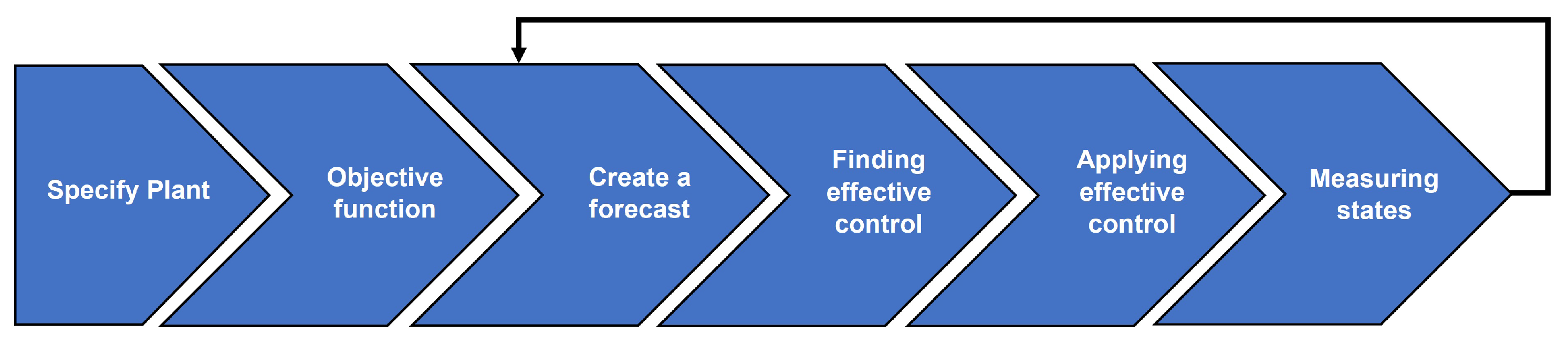The solution of this model is usually found by using classical optimality criteria, e.g., the Pontryagin’s maximum principle [6]. In this study, we focus on finding solutions that are robust to noise and take into account the dynamics of future changes in the process. We extend previous results by using a nonlinear model-predictive-control (MPC) controller to find effective controls [7]. MPC is a computational mathematical method used in dynamically controlled systems with observations to find effective controls.

It has been shown that several virus species, or several different virus strains of the same species, can circulate simultaneously in a population. In this case, the subpopulation of infected individuals can be divided into several subgroups. In our study, two types of virus were considered to simplify the calculations, but the results obtained can be generalized to a larger number of circulating strains.

Experience with influenza epidemics and the SARS-CoV-2 pandemic has shown that there can be several waves of illness in a population during a single epidemic season. To reduce the morbidity of an epidemic wave, the government and health authorities apply various measures to prevent and contain the epidemic. The use of different preventive and curative measures during a single wave reduces the number of cases and the rate at which the virus spreads in the population. Thus, the rise of the disease in the next wave of the epidemic begins with new initial states of the system. A review of the literature led to the idea of using predictive control models to develop effective control that takes into account changes in the environment. MPC controllers allow for the resulting control to be adapted by dividing the entire time interval into smaller sub-intervals. At each interval, the control system is checked to see if the constraints are satisfied, and if not, the control action is adjusted.

The main applications of this method are in the petrochemical [8], woodworking [9], and energy [10,11] industries, where, among other things, the stability of the obtained controllers and the possibility of their automatic adjustment are important. The MPC controller finds a solution in the form of piecemeal functions on the control interval, but the optimization problem is solved over a larger time interval—the forecast horizon. The MPC controller finds the solution in the form of piecewise constant functions on the control interval, but the optimization problem is solved on the forecast horizon.

As the main contribution of this work, we formulated a control problem and solved it using an MPC controller, a series of numerical experiments are carried out to confirm the effectiveness of the solutions obtained by the MPC controller for the SIIR model.

The paper is organized as follows. Section 2 presents the epidemic models and modified infection rate parameter. Section 3 shows the application of MPC-controllers to a SIIR epidemic model. In Section 4, we use numerical simulation to illustrate our results. The paper is concluded in Section 5.

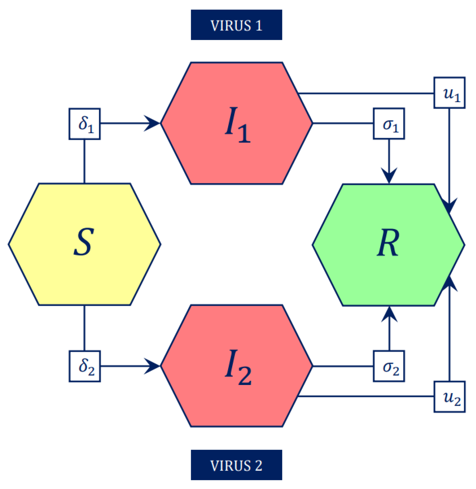
2. Epidemic Process in Total Urban Population

Our model is based on the extended Susceptible–Infected–Recovered model with two types of viruses, which circulate simultaneously in an urban population [6]. A size of population is equal to N. According to these assumptions, we can consider four groups: the Susceptible, the Infected by virus $V_1$, the Infected by virus $V_2$, and the Recovered group. Susceptible is a group of people who are not infected by viruses, but can be infected by one or both types of viruses and who have no immunity to the viruses. Depending on the viral strength, we observe that the number of people infected by virus 1 or by virus 2 can be different, and people infected by virus $V_1$ or $V_2$ belong to the subgroup Infected. The Recovered subgroup consists of people who have recovered from the infection. The mixing of populations allows for viruses to spread quickly, and each person in the population is assumed to have an equal probability of coming into contact with others. Therefore, when an infected person interacts with a susceptible person, the virus can spread. A virus with higher virulence, we assume, will have a higher probability of success in spreading when an encounter occurs between the infected and the susceptible. The scheme of process is represented in the Figure 1.

We model the spread of the virus in the population based on the classical SIR epidemiological model, where a system of differential equations is used to describe the proportion of the population as a function of time. Then, at time t, $n_S\left(t\right)$, $n_{I_1}\left(t\right)$, $n_{I_2}\left(t\right)$, and $n_R\left(t\right)$ correspond to the fractions of the population that are Susceptible, Infected by virus $v_1$, Infected by virus $v_2$, and Recovered, respectively, and for all t the condition $N=n_S\left(t\right)+n_{I_1}\left(t\right)+n_{I_2}\left(t\right)+n_R\left(t\right)$ is justified. Define $S\left(t\right)=\frac{n_S\left(t\right)}{N},I_1\left(t\right)=\frac{n_{I_1}\left(t\right)}{N},I_2\left(t\right)=\frac{n_{I_2}\left(t\right)}{N},R\left(t\right)=\frac{n_R\left(t\right)}{N}$ as proportions of Susceptible, Infected, and Recovered. At the beginning of the epidemic $t=0$, most people in the population belong to the susceptible subpopulation, a small group in the total population is infected and other people are in the recovered subpopulation. Therefore, initial states are $0<S\left(0\right)=S^0<1$, $0<I_1\left(0\right)=I_1^0<1$, $0<I_2\left(0\right)=I_2^0<1$, $R\left(0\right)=1-S^0-I_1^0-I_2^0$.

We have extended the simple SIR model introduced by [12] to describe the situation with two virus types:

$$\begin{array}{c}\dot{S}\left(t\right)=-{\mathsf{\delta }}_{1}S\left(t\right)I_1\left(t\right)-{\mathsf{\delta }}_{2}S\left(t\right)I_2\left(t\right);\hfill \\ \dot{I_1}\left(t\right)=({\mathsf{\delta }}_{1}S\left(t\right)-{\mathsf{\sigma }}_1-u_1\left(t\right))I_1\left(t\right);\hfill \\ \dot{I_2}\left(t\right)=({\mathsf{\delta }}_{2}S\left(t\right)-{\mathsf{\sigma }}_2-u_2\left(t\right))I_2\left(t\right);\hfill \\ \dot{R}\left(t\right)=({\mathsf{\sigma }}_1+u_1\left(t\right))I_1\left(t\right)+({\mathsf{\sigma }}_2+u_2\left(t\right))I_2\left(t\right);\hfill \end{array}$$

(1)

where ${\mathsf{\delta }}_i$ are infection rates for virus $V_i$, $i=1,2$, ${\mathsf{\sigma }}_i$ are recovery rates (see Figure 1). Infection rate is defined as a product of the contact rate l and transmissibility of infection, i.e., probability of transmission infection during the contact, ${\mathsf{\delta }}_{i_0}$

$${\mathsf{\delta }}_i=l{\mathsf{\delta }}_{i_0}\left(\frac{n_{I_i}}{N}\right).$$

Infection rate is integrated into the evolution of mutation process to epidemics in the urban population.

Medical treatment or quarantine reduces the number of the infected individuals in the urban population. These prevention measures can be interpreted as control parameters in the system defined as $u=(u_1,u_2)$; here, $u_i$ is a fraction of the infected which are quarantined or under intensive medical treatment. Recovered rates are inversely proportional to disease duration $\overline{T}$, hence ${\displaystyle {\mathsf{\sigma }}_i=\frac{1}{\overline{T}}}$.

The objective function: We will minimize the overall cost in time interval $[0,T]$ [13,14,15,16]. At any given t following costs exist in the system:

• $f_i\left(I_i\left(t\right)\right),i=\overline{1,2}$ is a function measuring the direct costs of infection, with a non-decreasing, twice differentiable function, such that $f_i\left(0\right)=0$, $f_i\left(I_i\left(t\right)\right)>0$ for $I_i\left(t\right)>0$. These costs can be interpreted as the price the government or medical organization pays for the health system to treat the infected and increase the probability of recovery for the treated individuals. Infected individuals who are not detected because they are asymptomatic are not treated, and therefore there are no direct costs for them.
• The treatment or medical cure of those infected produces costs for society. The functions $h_i\left(u_i\left(t\right)\right)$ represents the costs of treating the infected to keep them out of the labor market until recovery. The function $h_i\left(u_i\left(t\right)\right)$ is increasing on the argument $u_i\left(t\right)$, is twice differentiable, and is such that $h_i\left(u_i\left(0\right)\right)=0$.
• The function $g\left(R\right(t\left)\right)$ is a benefit rate. These are the bonuses that society receives from Recovered individuals who have returned to work and started contributing to society. The function $g\left(t\right)$ is non-decreasing and differentiable and $g\left(0\right)=0$.
• Constants $e_{I_1}$, $e_{I_2}$, $e_R$ represent the costs and benefit for Infected and Recovered in the end of the epidemic.

Aggregated system costs is given by

$$\begin{array}{c}{\displaystyle J=\underset{0}{\overset{T}{\int }}\left[f_1\left(I_1\left(t\right)\right)+f_2\left(I_2\left(t\right)\right)-g\left(R\left(t\right)\right)+h_1\left(u_1\left(t\right)\right)+h_2\left(u_2\left(t\right)\right)\right]dt+}\hfill \\ e_{I_1}{I}_1\left(T\right)+e_{I_1}{I}_2\left(T\right)-e_{R}R\left(T\right).\hfill \end{array}$$

(2)

and the optimal control problem is to minimize the cost, i.e.,

$$\underset{\{u_1,u_2\}}{min}J$$

To simplify the analysis, we consider the case where $e_{I_1}=e_{I_1}=e_R=0$.

Here, we assume that as a control parameters which help to reduce numbers of infected in human population, medical treatment or isolation can be considered, then define variable $u=(u_1,u_2)$ as control $0\le u_1\left(t\right)\le 1$, $0\le u_2\left(t\right)\le 1,$ for all t.

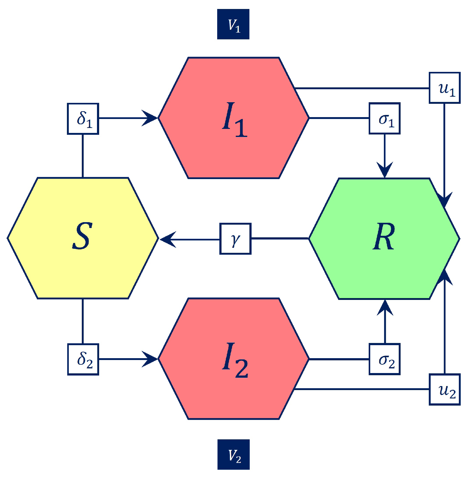
2.1. SIIRS Models

The SIIR models discussed in the previous section are best suited to describe epidemic processes in which viruses mutate slowly. Because of the small number of mutations, individuals can develop lifelong immunity to the virus. However, there are viruses that mutate rapidly and for these, SIIRS (Susceptible–Infected–Recovered–Susceptible) models have been developed (see Figure 2) to account for the decline of immunity in the population over time.

The system of differential equations describing the dynamics of state change is equal to

$$\left\{\begin{array}{c}\dot{S}\left(t\right)=\mathsf{\gamma }R\left(t\right)-{\mathsf{\delta }}_{1}S\left(t\right)I_1\left(t\right)-{\mathsf{\delta }}_{2}S\left(t\right)I_2\left(t\right),\hfill \\ \dot{I_1}\left(t\right)=({\mathsf{\delta }}_{1}S\left(t\right)-{\mathsf{\sigma }}_1-u_1)I_1\left(t\right),\hfill \\ \dot{I_2}\left(t\right)=({\mathsf{\delta }}_{2}S\left(t\right)-{\mathsf{\sigma }}_2-u_2)I_2\left(t\right),\hfill \\ \dot{R}\left(t\right)=({\mathsf{\sigma }}_1+u_1)I_1\left(t\right)+({\mathsf{\sigma }}_2+u_2)I_2\left(t\right)-\mathsf{\gamma }R\left(t\right).\hfill \end{array}\right.$$

(3)

Here, as in the SIIR model, the parameters ${\mathsf{\delta }}_i,{\mathsf{\sigma }}_i,i=\overline{1,2}$ are responsible for the intensity of infection and cure, $u_i$ —the proportion of infected people on medication, and $\mathsf{\gamma }$ —the intensity of immune decline in the population. The objective function for such tasks is no different from (2).

Note that due to the gradual decline of immunity, the epidemic process in the SIIRS problem can continue indefinitely. For this reason, when solving this problems we should choose large values for T. However, in such a case there is a risk (due to the high mutation rate of viruses) that the model parameters will no longer be relevant. Therefore, methods that can adapt to changes in the process by predicting its behavior can be effective in solving such problems.

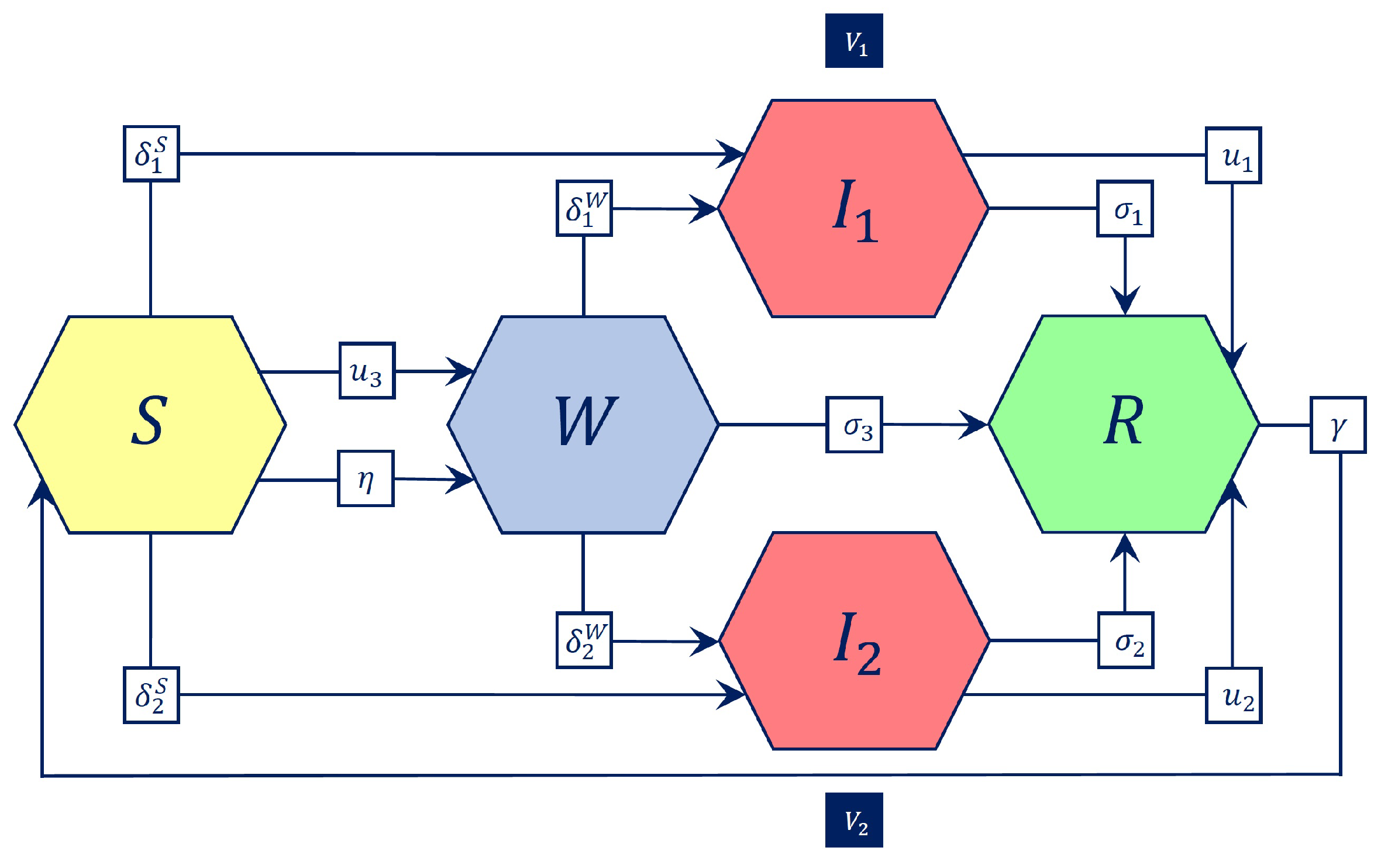
2.2. SWIIRS Model

In 2020, the SWIIRS (Susceptible–Warned–Infected–Recovered–Susceptible) model was proposed, which takes into account citizens’ awareness of the epidemic [17]. This model divides the population into five groups instead of four. An additional group of individuals is the group of warned W individuals who are aware of the virus (see Figure 3). This approach allows a more accurate description of epidemic processes in large countries, as the speed of spread of the virus often depends not only on the characteristics of the virus itself, but also on the behavior of members of the population.

The changes in population groups for the controlled SWIIRS model are described by a system of five differential equations:

$$\left\{\begin{array}{c}\dot{S}\left(t\right)=\mathsf{\gamma }R\left(t\right)-{\mathsf{\delta }}_1^{S}S\left(t\right)I_1\left(t\right)-{\mathsf{\delta }}_2^{S}S\left(t\right)I_2\left(t\right)-(\mathsf{\eta }W\left(t\right)+u_3)S\left(t\right),\hfill \\ \dot{W}\left(t\right)=(\mathsf{\eta }W\left(t\right)+u_3)S\left(t\right)-({\mathsf{\delta }}_1^W{I}_1\left(t\right)+{\mathsf{\delta }}_2^W{I}_2\left(t\right)+{\mathsf{\sigma }}_3)W\left(t\right),\hfill \\ \dot{I_1}\left(t\right)=({\mathsf{\delta }}_1^{S}S\left(t\right)+{\mathsf{\delta }}_1^{W}W\left(t\right)-{\mathsf{\sigma }}_1-u_1)I_1\left(t\right),\hfill \\ \dot{I_2}\left(t\right)=({\mathsf{\delta }}_2^{S}S\left(t\right)+{\mathsf{\delta }}_2^{W}W\left(t\right)-{\mathsf{\sigma }}_2-u_2)I_2\left(t\right),\hfill \\ \dot{R}\left(t\right)=({\mathsf{\sigma }}_1+u_1)I_1\left(t\right)+({\mathsf{\sigma }}_2+u_2)I_2\left(t\right)+{\mathsf{\sigma }}_{3}W\left(t\right)-\mathsf{\gamma }R\left(t\right).\hfill \end{array}\right.$$

(4)

In the system (4), the constants ${\mathsf{\delta }}_i^S$ and ${\mathsf{\delta }}_i^W$ describe the infection rates for groups S and W, respectively, and ${\mathsf{\sigma }}_i$– the cure rate $i=\overline{1,2}$. The value ${\mathsf{\sigma }}_3$ is responsible for the probability that a knowledgeable individual will acquire immunity to viruses (e.g., go to a health facility to get a vaccine). The intensity of the decline in immunity is described by $\mathsf{\gamma }$. Two parameters are responsible for informing (warning) members of the population:

• Parameter $u_3$—percentage of susceptible individuals informed by the media (become Warned);
• Parameter $\mathsf{\eta }$—probability of informing the susceptible individual when communicating with the warned individual.

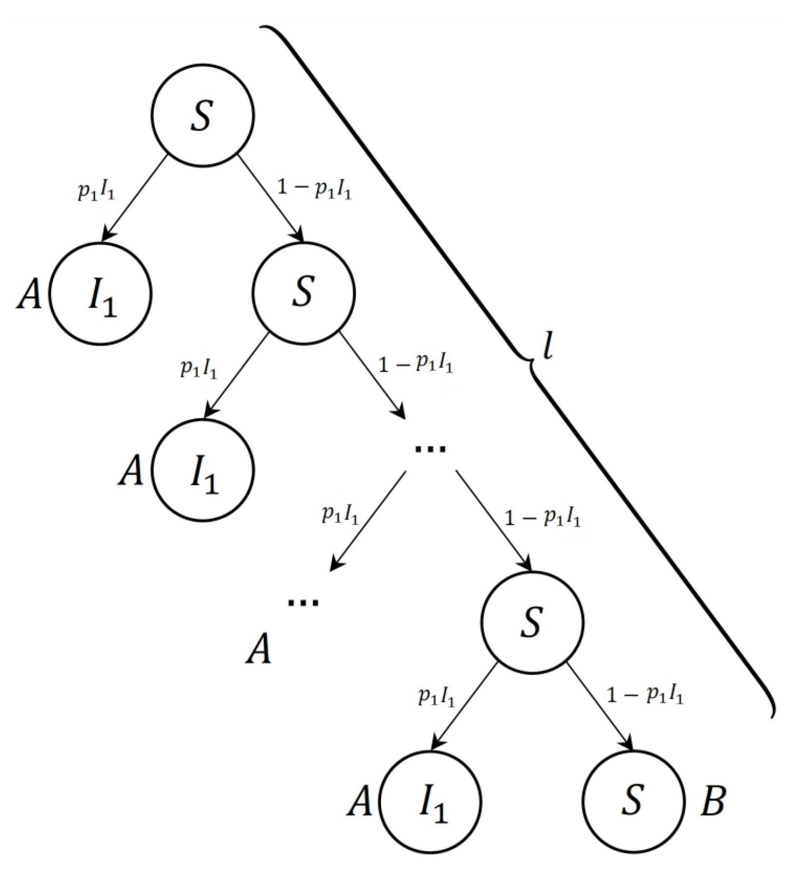
2.3. Controllable Infection Rate Parameter

Consider a model (1) with one virus $I_i$ and let $p_i$ be the probability of virus transmission $V_i$ from a diseased individual to a susceptible one, and l be the average number of contacts of an individual (with other members of the population) per unit of time. Consider a random contact of a susceptible individual. Infection with the virus will only occur if two events occur simultaneously: the contact was with the infected individual, and the virus was transmitted on contact.

Define two incompatible events:

• Event A— a susceptible individual becomes infected through one of an l contacts;
• Event B—with a similar number of contacts, infection will not occur.

Obviously that events A and B form a complete group of events (see Figure 4), then

$$p\left(A\right)+p\left(B\right)=1.$$

(5)

The event B will only occur if there is no infection at any of the l contacts. In other words

$$p\left(B\right)={\left(1-p_i{I}_i\left(t\right)\right)}^l.$$

(6)

From Equations (5) and (6) we see that the probability of transmission to a susceptible individual by l contact with infected individuals can be defined as

$$p\left(A\right)=1-{\left(1-p_i{I}_i\left(t\right)\right)}^l.$$

(7)

The same formula can be obtained in another way. The probability of the event A is given by

$$\begin{array}{c}p\left(A\right)=p_i{I}_i\left(t\right)+\left(1-p_i{I}_i\left(t\right)\right)p_i{I}_i\left(t\right)+{\left(1-p_i{I}_i\left(t\right)\right)}^2{p}_i{I}_i\left(t\right)+\\ {\displaystyle {\left(1-p_i{I}_i\left(t\right)\right)}^l{p}_i{I}_i\left(t\right)=\frac{p_i{I}_i\left(t\right)\left[{\left(1-p_i{I}_i\left(t\right)\right)}^l-1\right]}{-p_i{I}_i\left(t\right)}}\\ =1-{\left(1-p_i{I}_i\left(t\right)\right)}^l.\end{array}$$

(8)

This probability $p\left(A\right)$ is called the modified infection rate parameter and it is denoted by ${\tilde{\mathsf{\delta }}}_i(I_i\left(t\right),l)$.

Let us redefine $u_i(·)$ (intensive virus treatment) as $u_{i_1}(·)$. Let us introduce two types of control into the resulting system: isolation of infected individuals and reduction in the number of contacts in the whole system. Let $u_{i_2}(·)$ be the fraction of infected individuals isolated, and $u_l(·)$ be the fraction of contacts prevented by reducing the mobility of individuals in the whole population. In this case we obtain

$${\tilde{\mathsf{\delta }}}_i(I_i\left(t\right),l,u_{i_2}\left(t\right),u_l\left(t\right))={\left(1-p_i{I}_i\left(t\right)(1-u_{i_2}\left(t\right))\right)}^{l(1-u_l\left(t\right))},$$

(9)

where $0\le u_{i_2}\left(t\right),u_l\left(t\right)\le 1$. Then the system of differential equations of the corresponding single-variable SIR problem is

$$\left\{\begin{array}{c}\dot{S}\left(t\right)=-{\left(1-p_i{I}_i\left(t\right)(1-u_{i_2}\left(t\right))\right)}^{l(1-u_l\left(t\right))}S\left(t\right),\hfill \\ \dot{I_i}\left(t\right)={\left(1-p_i{I}_i\left(t\right)(1-u_{i_2}\left(t\right))\right)}^{l(1-u_l\left(t\right))}S\left(t\right)-({\mathsf{\sigma }}_1+u_{i_1}\left(t\right))I_i\left(t\right),\hfill \\ \dot{R}\left(t\right)=({\mathsf{\sigma }}_1+u_{i_1}\left(t\right))I_1\left(t\right).\hfill \end{array}\right.$$

(10)

If we perform similar transformations to (8) for the SIIR dual virus model, the calculated formulae for the controllable infection parameters are as follows

$$\begin{array}{c}{\tilde{\mathsf{\delta }}}_i={\tilde{\mathsf{\delta }}}_i(I_1\left(t\right),I_2\left(t\right),l,u_{1_2},u_{2_2},u_l)\\ {\displaystyle =\frac{p_i{I}_i\left(t\right)(1-u_{i_2})\left[{\left(1-p_1{I}_1\left(t\right)(1-u_{1_2})-p_2{I}_2\left(t\right)(1-u_{2_2})\right)}^{l(1-u_l)}-1\right]}{-p_1{I}_1\left(t\right)(1-u_{1_2})-p_2{I}_2\left(t\right)(1-u_{2_2})},}\end{array}$$

(11)

where $i=\overline{1,2}$. If we substitute these parameters into the system (1), the differential equations take the following form:

$$\left\{\begin{array}{c}\dot{S}\left(t\right)=-{\tilde{\mathsf{\delta }}}_{1}S\left(t\right)-{\tilde{\mathsf{\delta }}}_{2}S\left(t\right),\hfill \\ \dot{I_1}\left(t\right)={\tilde{\mathsf{\delta }}}_{1}S\left(t\right)-({\mathsf{\sigma }}_1+u_1)I_1\left(t\right),\hfill \\ \dot{I_2}\left(t\right)={\tilde{\mathsf{\delta }}}_{2}S\left(t\right)-({\mathsf{\sigma }}_2+u_2)I_2\left(t\right),\hfill \\ \dot{R}\left(t\right)=({\mathsf{\sigma }}_1+u_1)I_1\left(t\right)+({\mathsf{\sigma }}_2+u_2)I_2\left(t\right).\hfill \end{array}\right.$$

(12)

For the introduced controls we also need to redefine the cost functions. Let $h_{1_2}(u_{1_2},I_1)$, $h_{2_2}(u_{2_2},I_2)$, $h_l\left(u_l\right)$ be non-reducing functions corresponding to the costs of the controls $u_{1_2}$, $u_{2_2}$, and $u_l$. Then the function (2) takes the form

$$\begin{array}{c}\tilde{J}=\underset{0}{\overset{T}{\int }}[f_1\left(I_1\left(t\right)\right)+f_2\left(I_2\left(t\right)\right)-g\left(R\left(t\right)\right)+h_l\left(u_l\left(t\right)\right)+h_{1_1}\left(u_{1_1}\left(t\right)\right)+\\ h_{1_2}(u_{1_2}\left(t\right)+h_{2_1}\left(u_{2_1}\left(t\right)\right)+h_{2_2}\left(u_{2_2}\left(t\right)\right]dt.\end{array}$$

(13)

3. MPC Controllers

Model predictive control (MPC) is a set of methods for finding effective control based on model prediction. The basic idea of MPC is to estimate the future behavior of the controlled system at a finite time interval and to compute an effective control signal that minimizes a given objective function, given the constraints on the system (see Figure 5).

The next algorithm of the model-predictive-control method includes the following steps:

1.

Modeling of an object or process using mathematical and computer modeling techniques;

2.

Defining the main objectives to be achieved by management, selecting the forecasting horizon;

3.

Predicting the behavior of the process under the influence of the control signal;

4.

Find an effective control signal, taking into account the full range of constraints imposed on the control and manipulated variables;

5.

Select the control horizon in which the effective control found is applied;

6.

Measuring the actual process states at the end of the control horizon, which are taken as the new initial conditions;

7.

Shift the forecast horizon by the size of the management horizon and repeat steps 3–6.

3.1. Linear Prediction Model

We consider a linear controllable and observable finite-difference system:

$$\begin{array}{c}x(t+1)=A\left(t\right)x\left(t\right)+B\left(t\right)u\left(t\right),\hfill \\ y\left(t\right)=C\left(t\right)x\left(t\right),t\in [0,T],\hfill \end{array}u\left(t\right)\in U.$$

(14)

where $A\left(t\right)$, $B\left(t\right)$, $C\left(t\right)$ are some matrix functions of dimensions $n\times n$, $n\times m$, and $n\times k$, respectively, U is set of valid controls (is a subset of piecemeal functions), and $[0,T]$ is a given time interval.

Denote by $x_r$, $u_r$ the reference values of state and control variables. The MPC is a computational tool that finds the minimum either of its built-in target functionality (15) or of a custom function that the user must describe. Efficient control is determined using numerical Knows-What-It-Knows algorithms (KWIK) [18].

$$\underset{0}{\overset{T}{\int }}\langle w_x,{(x-x_r)}^2\rangle +\langle w_u,{(u-u_r)}^2\rangle dt,t\in [0,T],$$

(15)

where $w_x$ and $w_u$ weight vectors for variables x and u. However, the system (1) should be transformed to have a possibility to apply the MPC controller. In our case we find a control $u\left(t\right)$ that provides the minimum to the objective function (2). The system (1) must be linearized before the MPC can be used. The predicted values are determined by the formula:

$$\overline{y}=Gx\left(t\right)+Hv+Fu\left(t\right),\mathrm{where}$$

(16)

• $x\left(t\right),u\left(t\right)$—the known current states and controls of the system,
• $\overline{y}=\left(\begin{array}{c}\overline{y}(t+1)\\ \overline{y}(t+2)\\ ...\\ \overline{y}(t+N)\end{array}\right)$—model prediction,
• $v=\left(\begin{array}{c}v(t+1)\\ v(t+2)\\ ...\\ v(t+N)\end{array}\right)$—planned control signals,
• $H=\left(\begin{array}{cccc}0& 0& ...& 0\\ CB& 0& ...& 0\\ ...& ...& ...& ...\\ C{A}^{N-2}B& C{A}^{N-3}B& ...& 0\end{array}\right)$,
• $G=\left(\begin{array}{c}CA\\ C{A}^2\\ ...\\ C{A}^N\end{array}\right)$,
• $F=\left(\begin{array}{c}CB\\ CAB\\ ...\\ C{A}^{N-1}B\end{array}\right)$.

The solution of the obtained problem is carried out using standard methods for solving quadratic programming problems. Let

$$v^{*}=\left(\begin{array}{c}{v}^{*}(t+1)\\ v^{*}(t+2)\\ ...\\ v^{*}(t+N)\end{array}\right)$$

(17)

solution of the problem (15), then $v^{*}(t+1)$ will be called the effective control for the original system (14) on the interval $[t,t+1]$ obtained using MPC method. After applying the control, we obtain the new initial data $x(t+1)$ and $u(t+1)$ to make the following forecast and search for an effective control on the interval $[t+1,t+2]$.

3.2. Linearization of $S{I}_1{I}_{2}R$ Problem

In the current section, we discuss the application of the MPC controller to the extended $S{I}_1{I}_{2}R$ system [19].

Suppose, that the initial states for all states $S\left(0\right),I_1\left(0\right),I_2\left(0\right),R\left(0\right)$ are known. Otherwise, we can always measure it. Define $SIIR\left(0\right)$ as a vector of initial states.

$$S{I}_1{I}_{2}R\left(0\right)=\left(\begin{array}{c}{S}^0\\ I_1^0\\ I_2^0\\ R^0\end{array}\right).$$

(18)

Another assumption is that the initial control $u\left(0\right)=u^0$ is defined. We divide the initial period of time $[0,T]$ into k equal parts, then the objective function (2) by the integral property can be written as:

$$\begin{array}{c}J=\underset{0}{\overset{T}{\int }}[f_1\left(I_1\left(t\right)\right)+f_2\left(I_2\left(t\right)\right)-g\left(R\left(t\right)\right)+h_1\left(u_1\left(t\right)\right)+h_2\left(u_2\left(t\right)\right)]dt\\ =J_1+\dots +J_k,\mathrm{where}\\ J_i=\underset{T_{i-1}}{\overset{T_i}{\int }}[f_1\left(I_1\left(t\right)\right)+f_2\left(I_2\left(t\right)\right)-g\left(R\left(t\right)\right)+h_1\left(u_1\left(t\right)\right)+h_2\left(u_2\left(t\right)\right)]dt.\end{array}$$

(19)

Here, the total length of time interval is divided into several segments ${\displaystyle [T_{i-1},T_i]}$, where ${\displaystyle T_{i-1}=\frac{(i-1)T}{k}}$ and $T_i=\frac{iT}{k}$, $i=\overline{1,k}$.

Obviously, that $\underset{u\in U}{min}{J}_1+\underset{u\in U}{min}{J}_2+...+\underset{u\in U}{min}{J}_k\le \underset{u\in U}{min}J$. Then, instead of the original problem, we consider k-th sub-interval with objective function of the form (20), taking into account the system (1):

$$J_i\to \underset{u\in U}{min}.$$

(20)

The initial conditions for the first iteration are defined in (18), for each subsequent problem they can be found from the previous task as:

$$S{I}_1{I}_{2}R\left(T_i\right)=\left(\begin{array}{c}S\left(T_i\right)\\ I_1\left(T_i\right)\\ I_2\left(T_i\right)\\ R\left(T_i\right)\end{array}\right)=\left(\begin{array}{c}{S}^i\\ I_1^i\\ I_2^i\\ R^i\end{array}\right),u^i=u\left(T_i\right),i=\overline{1,k-1}-\mathrm{iteration}\mathrm{number}.$$

(21)

Let us redefine $S{I}_1{I}_{2}R\left(t\right)=\left(\begin{array}{c}S\left(t\right)\\ I_1\left(t\right)\\ I_2\left(t\right)\\ R\left(t\right)\end{array}\right)$ as a vector $x\left(t\right)=\left(\begin{array}{c}{x}_1\left(t\right)\\ x_2\left(t\right)\\ x_3\left(t\right)\\ x_4\left(t\right)\end{array}\right)$. The system (1) is also valid for initial values, i.e.,

$$\begin{array}{c}{\dot{x}}_1^i=f_1(x^i,u^i,t)=-({\mathsf{\delta }}_1{x}_2^i+{\mathsf{\delta }}_2{x}_3^i)x_1^i;\hfill \\ {\dot{x}}_2^i=f_2(x^i,u^i,t)=({\mathsf{\delta }}_1{x}_1^i-{\mathsf{\sigma }}_1-u_1^i)x_2^i;\hfill \\ {\dot{x}}_3^i=f_3(x^i,u^i,t)=({\mathsf{\delta }}_2{x}_1^i-{\mathsf{\sigma }}_2-u_2^i)x_3^i;\hfill \\ {\dot{x}}_4^i=f_4(x^i,u^i,t)=({\mathsf{\sigma }}_1+u_1^i)x_2^i+({\mathsf{\sigma }}_2+u_2^i)x_3^i.\hfill \end{array}$$

(22)

Consider some disturbance of this system:

• $\tilde{x}\left(t\right)=x^i\left(t\right)+\Delta x\left(t\right)$, where $\Delta x\left(t\right)$—state variable variation vector;
• $\tilde{u}\left(t\right)=u^i\left(t\right)+\Delta u\left(t\right)$, where $\Delta u\left(t\right)$—control variable variation vector.

Then, ${\dot{x}}^i\left(t\right)+\Delta \dot{x}\left(t\right)=f(\tilde{x},\tilde{u},t)$. The right hand sides of system (22) is decomposed into a Taylor row:

$$\begin{array}{c}{\dot{x}}^i\left(t\right)+\dot{\Delta x}\left(t\right)\\ {\displaystyle =f(x^i\left(t\right),u^i\left(t\right),t)+\frac{df}{dx}{|}_{x^i,u^i}\Delta x\left(t\right)+\frac{df}{du}{|}_{x^i,u^i}\Delta u\left(t\right)+O({(\Delta x)}^2,{(\Delta u)}^2).}\end{array}$$

(23)

Here, $O({(\Delta x)}^2,{(\Delta u)}^2)$ is the second-order residual term of smallness. Subtract from (22) and obtain

$$\dot{\Delta x}\left(t\right)=\underset{A^i\left(t\right)}{\underbrace{\frac{df}{dx}{|}_{x^i,u^i}}}\Delta x\left(t\right)+\underset{B^i\left(t\right)}{\underbrace{\frac{df}{du}{|}_{x^i,u^i}}}\Delta u\left(t\right).$$

(24)

As a result, the linearized controlled system is obtained. We substitute the solution $(\overline{x},\overline{u})$ of the linearized system into the original model (1), (20) and obtain the following value of the objective function $J_i(\overline{x},\overline{u})={\overline{J}}_i$. Let $(x^{*},u^{*})$ be a solution that provides a minimum to the functional (20), then we can denote by an error in the solution the value of the ${\mathsf{\epsilon }}_i$, which is determined by the formula:

$${\mathsf{\epsilon }}_i=|J_i(\overline{x},\overline{u})-J_i(x^{*},u^{*})|,i=\overline{1,k}.$$

(25)

Going to the limit $k\to \infty$, we have:

$$\underset{k\to \infty }{lim}{\dot{x}}^i=A^{i}x+B^{i}u=>\underset{k\to \infty }{lim}(\overline{x},\overline{u})=(x^{*},u^{*})=>\underset{k\to \infty }{lim}{\mathsf{\epsilon }}_i=0.$$

(26)

This means that the greater the number of split points, the more accurate the solution will be.

We have conducted a series of numerical simulations to check whether the MPC controller solution converges to the optimal solution as the parameter k increases (the other parameters remain the same). It can be seen that all the costs (standard, efficient, and optimal) increase as k increases. This is due to the fact that the accuracy of the integral calculation in the function increases. In test no. 2, the value of the effective costs is extremely high, due to the fact that it is recommended to use the value $k\ge T$. Starting from test no. 5, the values of effective costs and optimal costs differ insignificantly, so in practice we use the values $k=2T$ or $k=4T$. However, the program execution time in the second case (test no. 9) is 10 times longer than in the first case (test no. 5).

3.3. Nonlinear MPC-Controller

Figure 6 shows the work of the nonlinear MPC controller [20]. The MPC controller construct the efficient control ${\left(u^{*}\right)}^i$ and predictive values of the objective function using a vector of outputs $y^i$ of the system. The main difference between nonlinear and linear MPC controller is the linearization of the optimization problem before the application of the solver [21,22].

The received control is inputted to the dynamic system, in the next iteration MPC-controller obtains another output. The process of constructing a solution is complete when the control horizon is reached. The final effective control strategy is chosen to minimize the objective function on the predictive horizon. Since numerical algorithms are used to find the solution, the resulting effective value can be suboptimal.

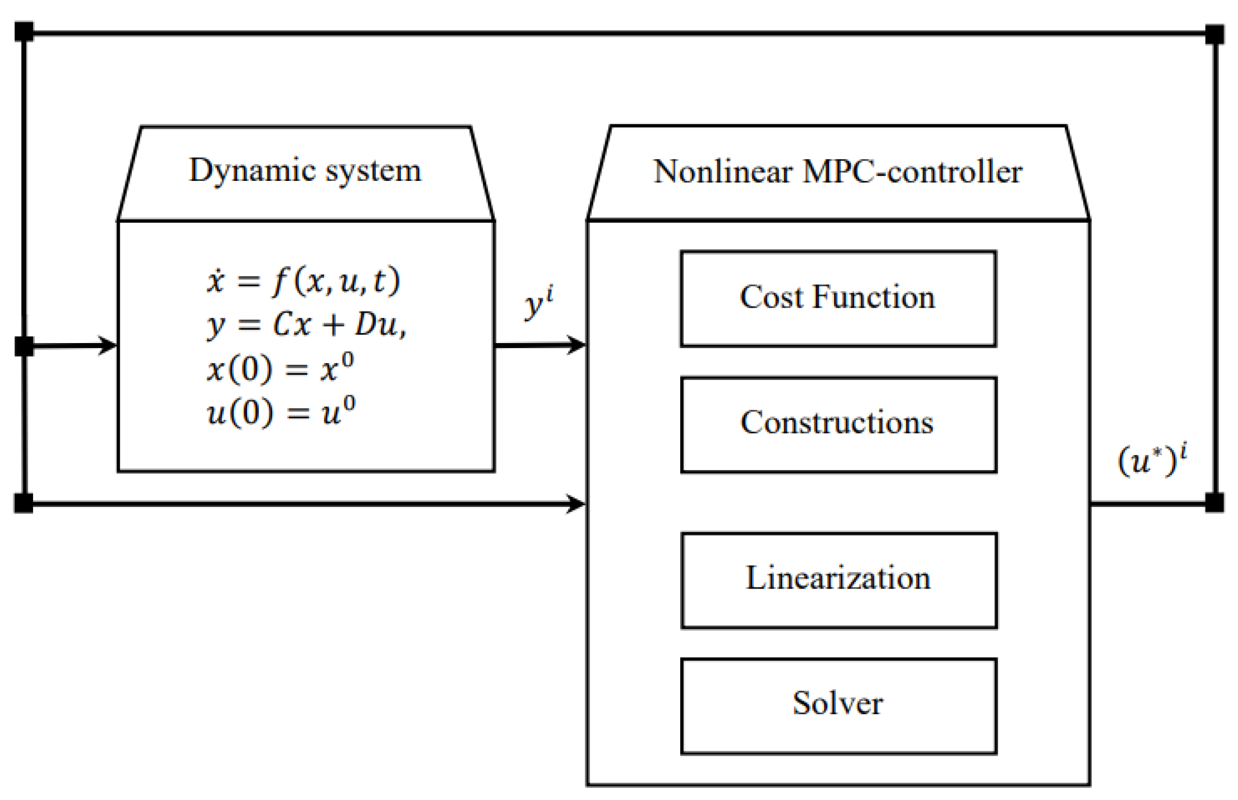
4. Numerical Simulations

This section presents the results of a numerical simulation that corroborates our theoretical results. The numerical experiments are aimed at obtaining effective treatment strategies using nonlinear MPC controllers. We selected MATLAB as our platform for programming and numerical calculations for a series of experiments. MATLAB offers an extensive library of the model-predictive-control method, including various examples. Nonlinear-MPC controllers were employed in our study. These controllers utilize the linearization algorithm described in the article to find solutions. Nonlinear MPC is adequate to address these issues. However, larger systems may demand more precise predictive models based on machine learning and neural networks. For first three experiments, two variants of the SARS-CoV-2 virus were selected for study: Alpha [23] and Omicron [24]. The epidemic situation was considered for a period of 180 days (6 months). During this period, six MPC controllers were used sequentially with a forecast horizon of 30 days (1 month) and a control horizon of 21 days (3 weeks). Time dependence of MPC controller accuracy and performance on k parameter are shown in

Table 1. Dependence of MPC controller accuracy and performance on k parameter.

Test	T	k	Standard Costs	Effective Costs	Optimal Cost	Operation Time
1	180	60	4264	825	803	5.31 s
2	180	90	4273	1017	817	9.64 s
3	180	120	4278	851	839	9.17 s
4	180	180	4282	860	856	15.00 s
5	180	360	4286	866	865	1 min 0.72 s
6	180	450	4286	868	867	1 min 58.87 s
7	180	540	4287	870	870	4 min 6.98 s
8	180	630	4287	870	870	6 min 20.63 s
9	180	720	4287	870	870	10 min 16.43 s

. The values of the main system parameters are shown in

Table 2. Values of system parameters and initial states for Experiments 1, 2, and 3.

Parameter	Value	Characteristics
Dynamic System Settings
n	4	Number of system states
r	4	Number of system outputs
m	2	Number of control variables
Time parameters
$Tl$	6	Number of time intervals
$Ts$	0.25	Step of the controller
$PH$	30	Prediction Horizon
$CH$	21	Control Horizon
Parameters of the $SIIR$ model
	1 (Exp. 1)	Average number of contacts per day
k	3 (Exp. 2)	(Exp. stands for Experiment)
	10 (Exp. 3)
Virus 1 (SARS-CoV-2 Alpha)
${\mathsf{\delta }}_1$	0.256	Infection rate of Virus 1
${\mathsf{\sigma }}_1$	0.025	Recovery rate of Virus 1
Virus 2 (SARS-CoV-2 Omicron)
${\mathsf{\delta }}_2$	0.517	Infection rate of Virus 2
${\mathsf{\sigma }}_2$	0.07	Recovery rate of Virus 2
Cost function parameters
$f_1$	134.5	Infection costs for virus 1
$f_2$	134.5	Infection costs for virus 2
$h_1$	192.07	Treatment costs for virus 1
$h_2$	192.07	Treatment costs for virus 2

.

The serial application of multiple nonlinear MPC controllers allows the constraints, system parameters and objective function coefficients to be adjusted step by step. To simplify the calculations, we will use the same parameters in each iteration of the process.

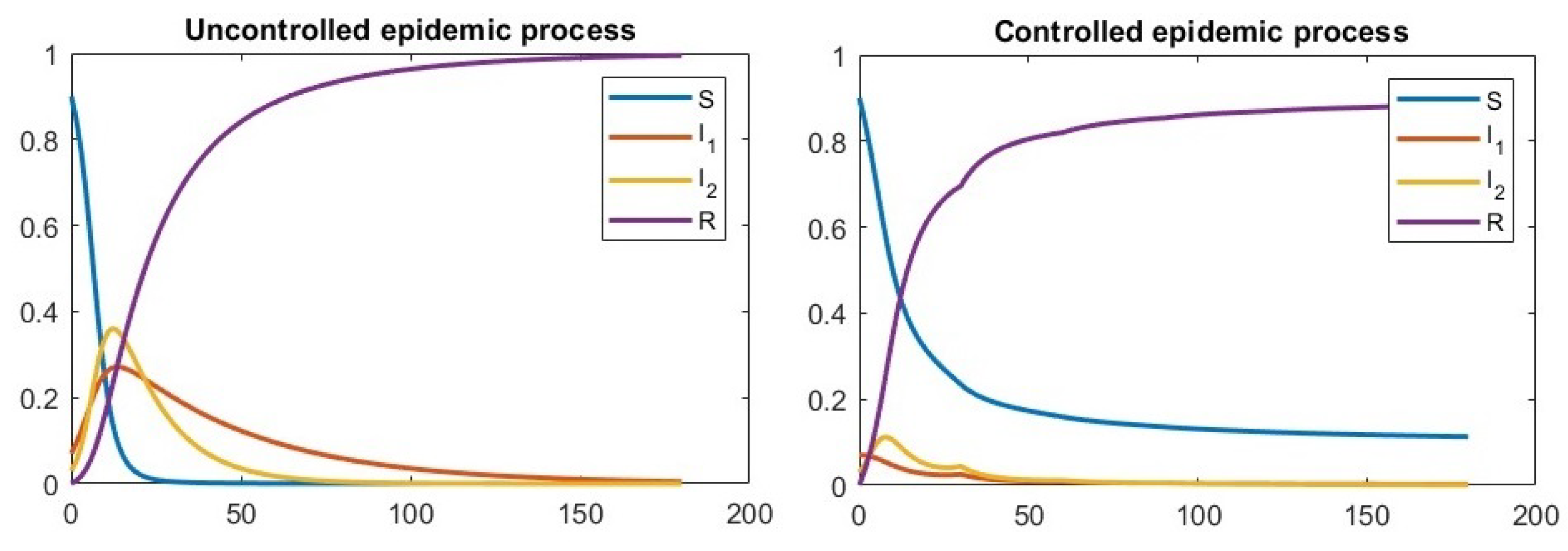
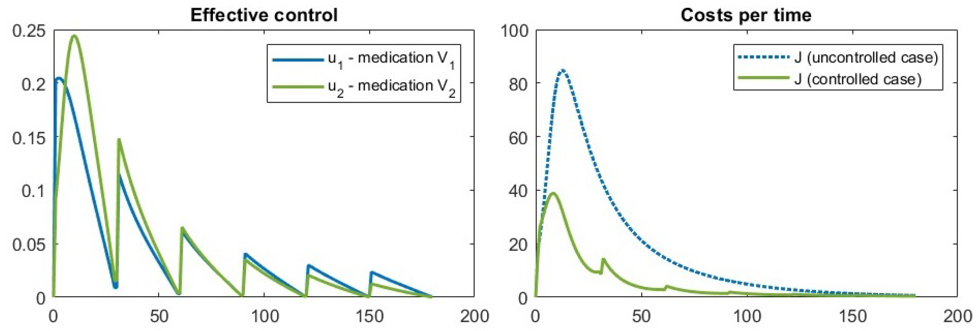
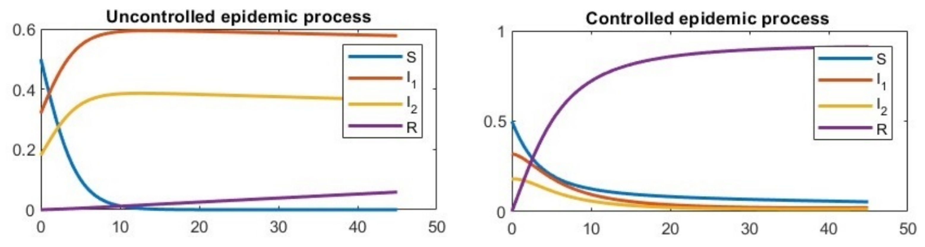
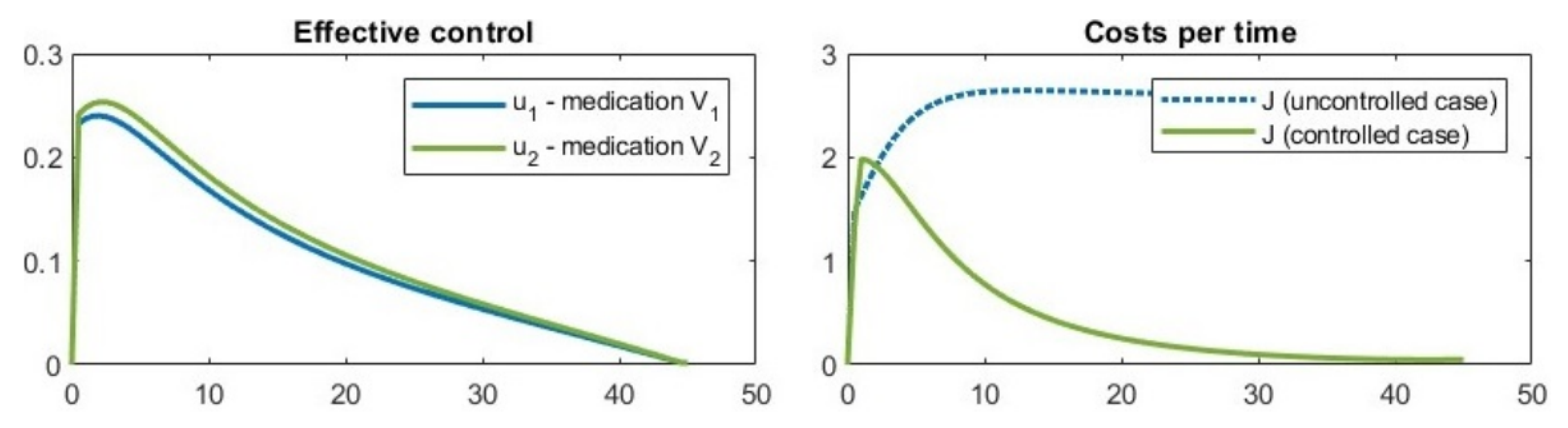
Experiment 1. In the first experiment, we considered the epidemic process with a small number of contacts, which is possible in cases where most of the infected comply with the quarantine. It can be seen that applying control is having a positive impact on stopping the virus spreading (Figure 7). On the effective control graph (Figure 8), you can notice “jumps” due to the fact that a new MPC controller is connected each new month (30th day). However, the resulting control greatly reduces the damage from the epidemic compared to a situation where we do not control the epidemic process. So the cost in the uncontrolled case is $J_0=3159$ monetary units (m.u.) and with the effective strategy $J_{eff}=1016$ m.u. The benefit of using control is therefore 2143 m.u.

Experiment 2. A second experiment (Figure 9 and Figure 10) was run with the average number of contacts per day $k=3$. This experiment is the most different from the others. The main wave of the epidemic does not occur in the first few days, but only at the beginning of the third month. The highest costs are in the same period. After $t=60$, the effective control is similar to that of experiments 1 and 3. With this strategy, it is possible to reduce the cost of the epidemic from $J_0=3613$ m.u. to $J_{eff}=1045$ m.u., which saves 2568 monetary units.

It can also be seen that as the average number of contacts increased, so did the values of the objective functions. Just as importantly, the benefits of using MPC controllers have also increased.

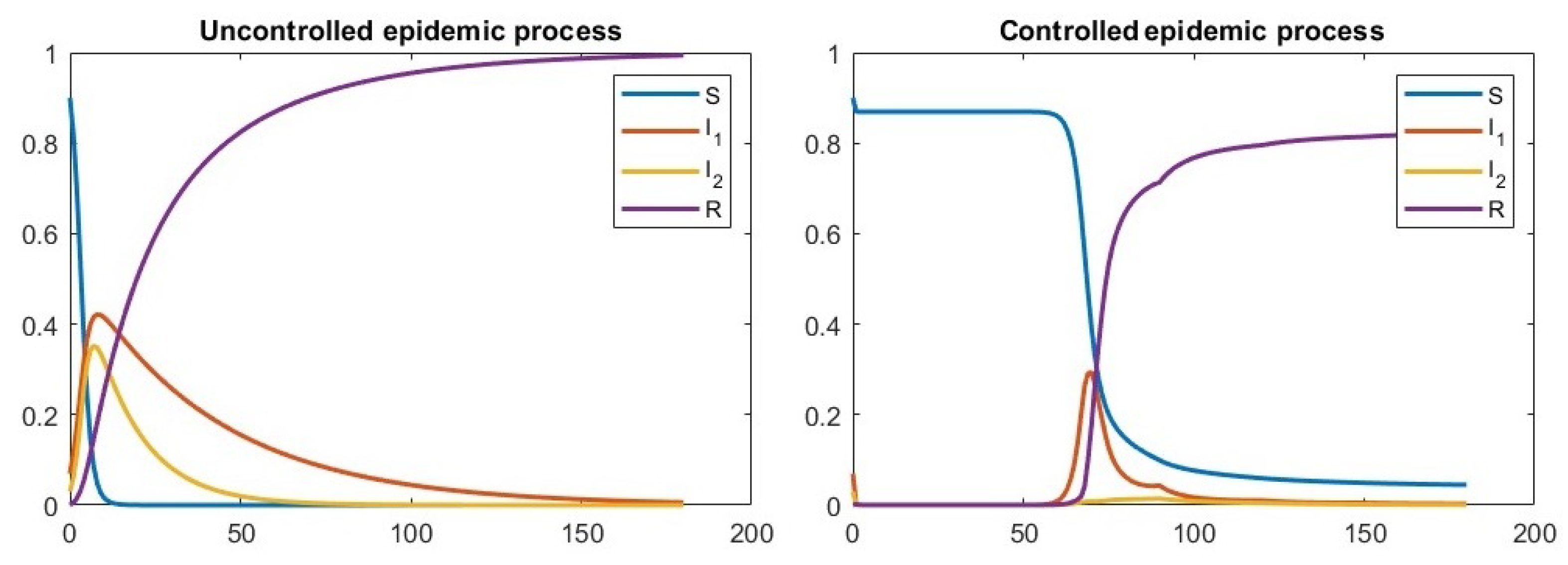
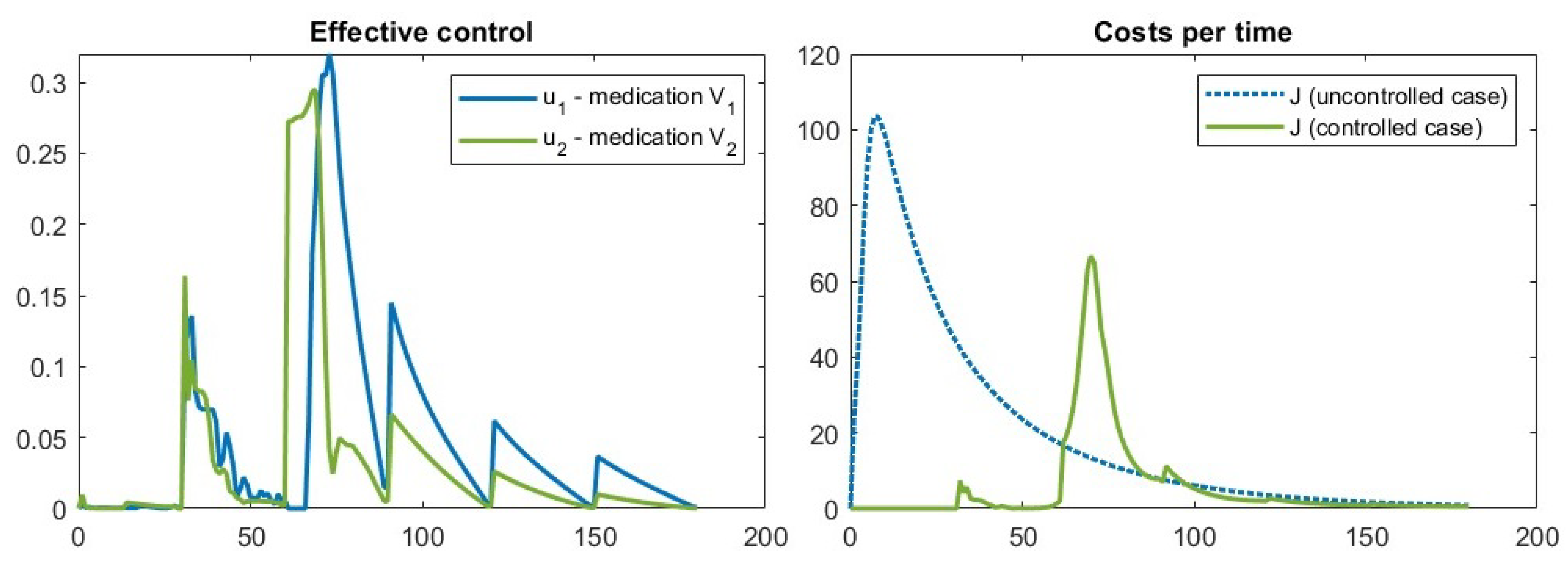
Experiment 3. In the third simulation the number of contacts is $k=10$, which approximates the real situation. Figure 11 shows that with a large number of contacts, almost all agents are infected by $t=5$. However, when efficient control is used, the infection peaks are significantly reduced (from $0.63$ to $0.29$ and from $0.26$ to $0.14$). As in the previous experiments, the use of efficient control is economically beneficial, reducing costs from $J_0=4282$ m.u. to $J_{eff}=860$ m.u. The benefit of using an effective strategy is 3422 m.u. (see Figure 12).

It should also be noted that despite the largest value of k the costs of using effective management in Experiment 3 turned out to be the smallest. This may be due to the fact that when solving the problem, they are linearized and the accuracy of the solution can vary from the parameters of the problem. At the same time, all three experiments showed that effective control can reduce the economic damage from the epidemic, which shows the practical importance of using the model predictive control in SIIR problem.

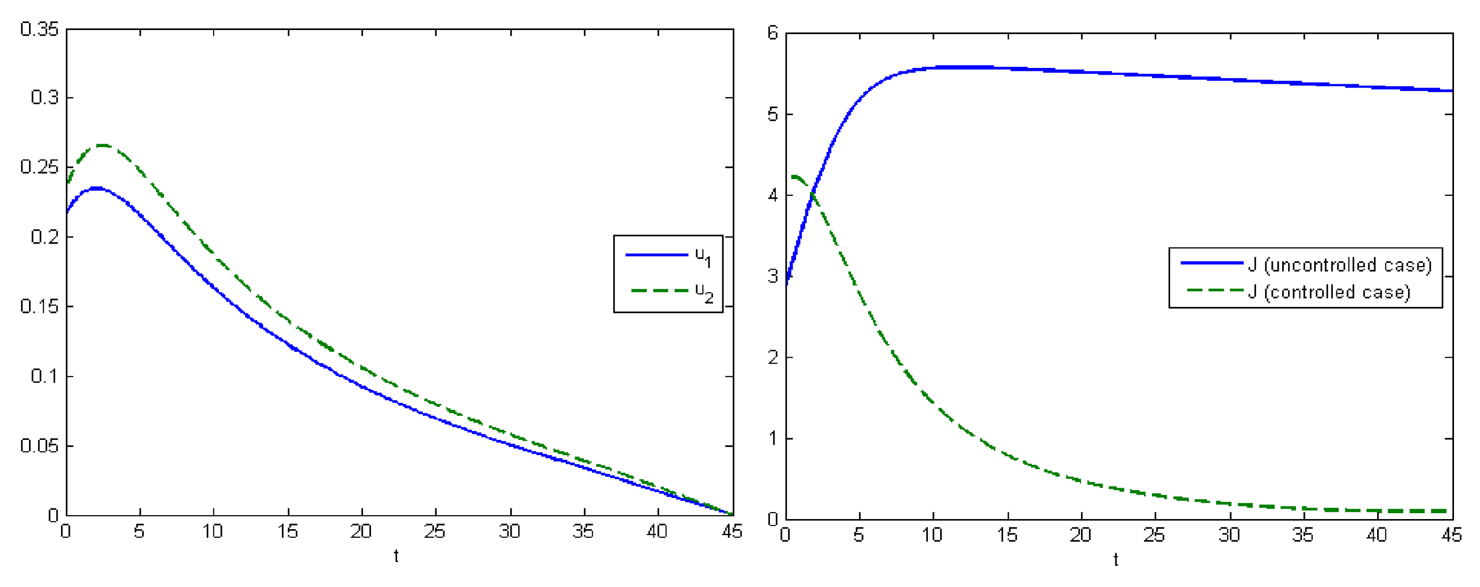
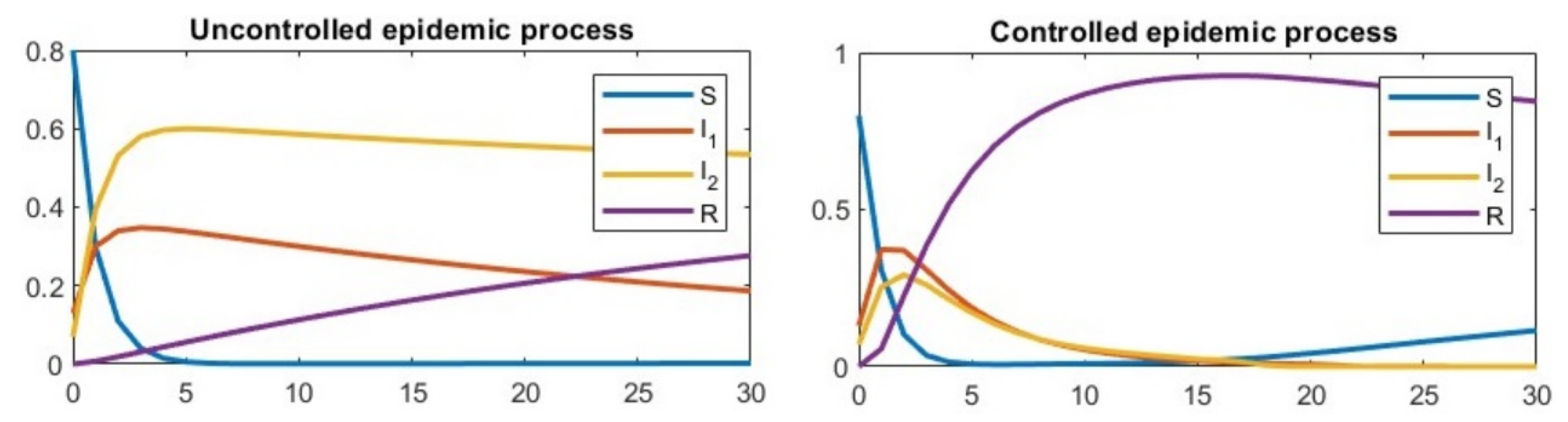
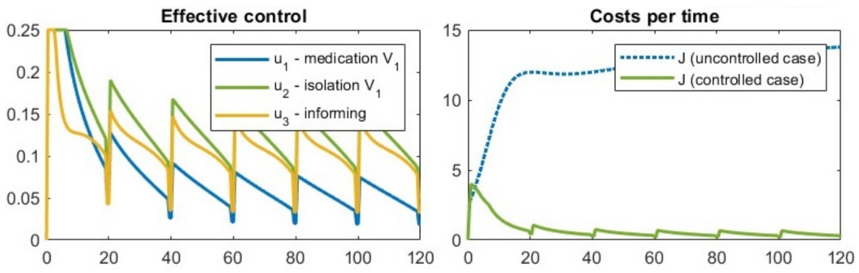
Experiment 4. In the fourth experiment we examined the SIIR model with the data taken from the paper “Optimal control of heterogeneous mutating viruses” [5].

Table 3. Values of system parameters and initial states for Experiment 4.

Parameter	Value	Description
Characteristics of the virus
${\mathsf{\delta }}_1$	$0.4$	Infection rate of $V_1$
${\mathsf{\delta }}_2$	$0.5$	Infection rate of $V_2$
${\mathsf{\sigma }}_1$	$0.001$	Recovery rate from $V_1$
${\mathsf{\sigma }}_2$	$0.002$	Recovery rate from $V_2$
Cost functions
$f_1\left(I_1\right)$	$5I_1$	Infection costs of $V_1$
$f_2\left(I_2\right)$	$6I_2$	Infection costs of $V_2$
$g\left(R\right)$	$0.1R$	Benefit rate
$h_1\left(u_1\right)$	$15u_1^2$	Cost of treatment $u_1$
$h_2\left(u_2\right)$	$10u_2^2$	Cost of treatment $u_2$
Initial states
$S\left(0\right)$	$0.50$	Fraction of Susceptible
$I_1\left(0\right)$	$0.32$	Fraction of Infected with $V_1$
$I_2\left(0\right)$	$0.18$	Fraction of Infected with $V_2$
$R\left(0\right)$	$0.00$	Fraction of Recovered
Values of MPC controller
$Tl$	1	Number of time intervals
$Ts$	$0.5$	Step of the controller
$PH$	90	Prediction horizon
$CH$	90	Control horizon

shows the parameter values used in the simulation.

Figure 13 shows the population states in the uncontrolled and controlled cases. It can be seen that the use of the control found with MPC significantly reduces the number of infections. In the uncontrolled case, the maximum proportion of the number of infections is $I_{1_{max}}=0.594$, $I_{2_{max}}=0.386$, and in the controlled case, $I_{1_{max}}=0.32$, $I_{2_{max}}=0.18$, corresponding to the initial proportion of infected in the population.

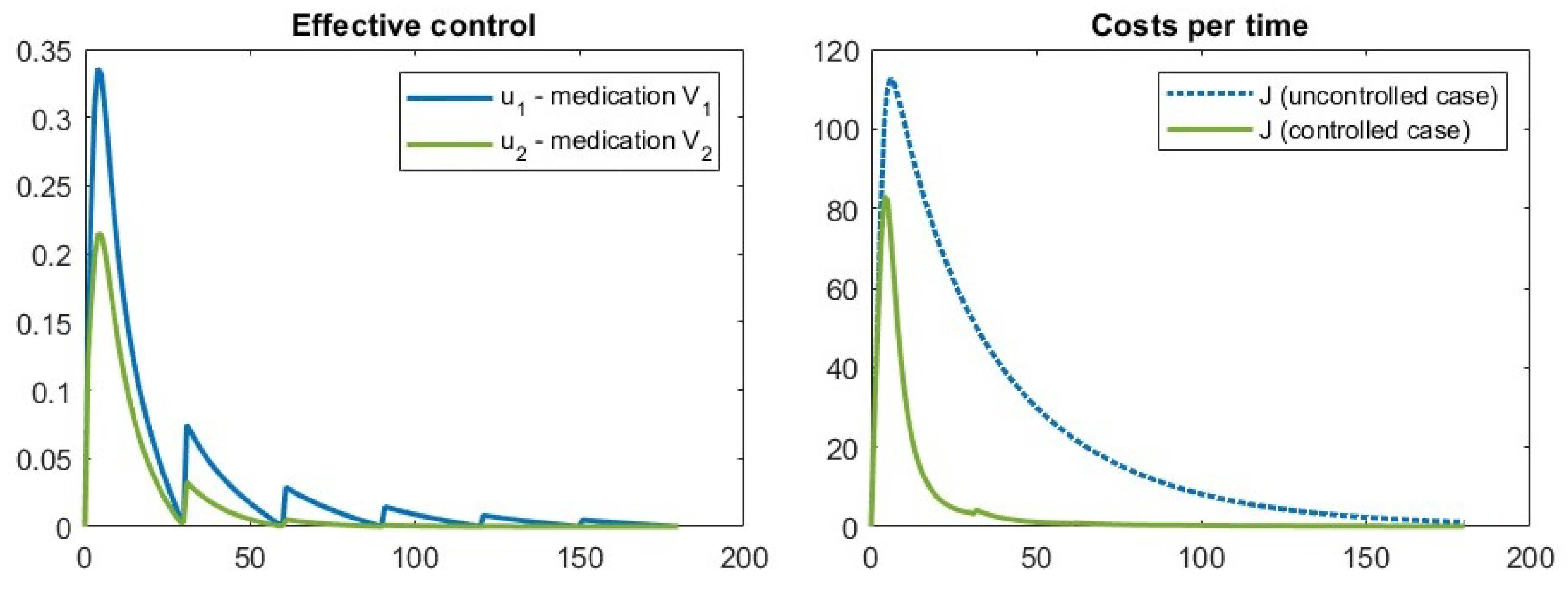
After the computer simulation, the solution of the formulated problem was obtained and the values of the functional were found (see Figure 14).

The strategies that increased to $u_1=0.26$ and $u_2=0.24$ during the first three days of the epidemic and then decreased to zero were found to be effective. The resulting control signals are similar in appearance to the continuous controls presented in the experiments of this paper. The aggregated costs are equal to $41.6$ m.u. in the controlled case and $227.51$ m.u. in the uncontrolled case. Thus, the benefit of using the control is $185.91$ monetary units, which is slightly less than using the optimal control $189.17$ m.u. In Figure 15, we can see the structure of the optimal control for the model and the data from this experiment. It can be observed that the control structure in the case of effective control is similar to the structure in the case of optimal control.

Experiment 4 showed that the developed software package finds near-optimal solutions to classical SIIR problems and can be used as an alternative to classical optimal control methods.

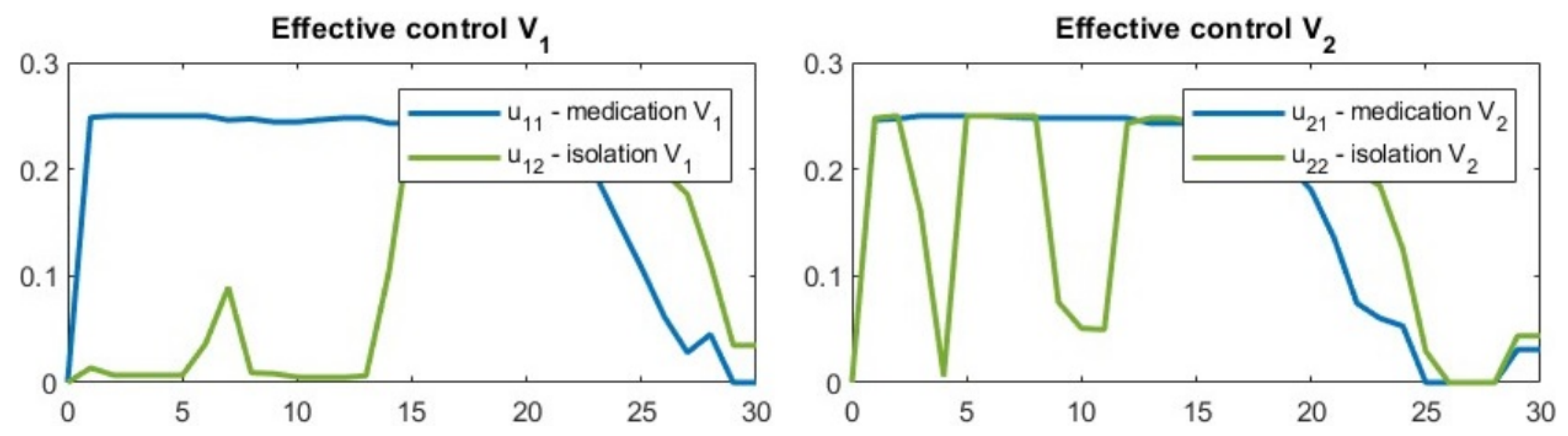
Experiment 5. As the software implementation of the MPC method showed good accuracy for standard tasks, Experiment 5 was conducted using a modified SIIRS model (with controlled infection rate parameter). Data for the experiment were obtained from sources such as the World Health Organization, Our World in Data, and Worldometer. The parameters of the experiment are shown in

Table 4. Values of system parameters and initial states for Experiment 5.

Parameter	Value	Description
Characteristics of the virus
$p_1$	$0.256$	Infection probability with virus $V_1$ (single contact)
$p_2$	$0.517$	Infection probability with virus $V_2$ (single contact)
${\mathsf{\sigma }}_1$	$0.025$	Recovery rate from $V_1$
${\mathsf{\sigma }}_2$	$0.007$	Recovery rate from $V_2$
$\mathsf{\gamma }$	$1/120\approx 0.0083$	Decreasing immunity rate
l	30	Average number of contacts in the population
$f_1\left(I_1\right)$	$135I_1$	Infection costs of $V_1$
$f_2\left(I_2\right)$	$135I_2$	Infection costs of $V_2$
$g\left(R\right)$	0	Benefit rate
$h_{1_1}\left(u_{1_1}\right)$	$192{\left(u_{1_1}\right)}^2$	Treatment cost $u_{1_1}$
$h_{1_2}(u_{1_2},I_1)$	$94u_{1_2}{I}_1$	Isolation cost $u_{1_2}$
$h_{2_1}\left(u_{2_1}\right)$	$192{\left(u_{2_1}\right)}^2$	Treatment cost $u_{2_1}$
$h_{2_2}(u_{2_2},I_2)$	$94u_{2_2}{I}_2$	Isolation cost $u_{2_2}$
$h_l\left(u_l\right)$	$94{\left(u_l\right)}^2$	Cost of reducing the number of contacts $u_l$
Initial states
$S\left(0\right)$	$0.8$	Fraction of Susceptible
$I_1\left(0\right)$	$0.13$	Fraction of Infected with $V_1$
$I_2\left(0\right)$	$0.07$	Fraction of Infected with $V_2$
$R\left(0\right)$	$0.00$	Fraction of Recovered
Values of MPC controller
k	1	Number of controllers
$Ts$	$0.5$	Step the controller
$PH$	45	Forecast horizon
$CH$	30	Control horizon

.

Using effective strategies (see Figure 16), it was possible to reduce the maximum proportion infected with $V_2$ virus from $0.6$ to $0.3$, but the proportion infected with $V_1$ virus increased from $0.34$ to $0.38$, which is due to the fact that the proportion of people (30% of the population) who were not infected with $V_2$ virus (due to the measures introduced) managed to become infected with $V_1$ virus. It can also be seen that from $t=15$, the proportion infected with both viruses does not exceed 1%.

By running the computer simulation program, effective controls for the formulated problem were obtained (see Figure 17). It can be observed that the treatment of individuals for both viruses takes a maximum value starting from $t=1$ and decreases for virus $V_1$ after $t=21$ and for virus $V_1$ after $t=18$. For $V_1$, a small fraction ($u_{1_2}=0.1$) of those infected during $[5,8]$ are isolated, and after $t=15$ the control $u_{1_2}$ turns on again, reaching a maximum value, and turns off after $t=24$. For $V_2$, maximum isolation of the infected occurs at $[0,4]$, $[5,8]$, $[12,21]$, and partial isolation at $[9,11]$, $[29,30]$. 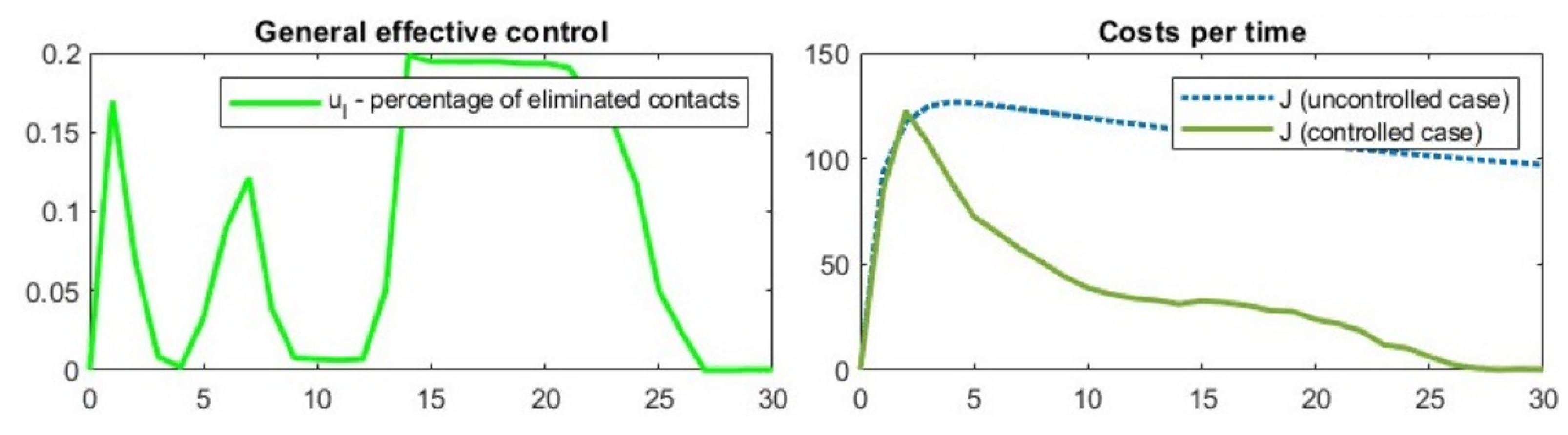Reducing the total number of contacts was most effective in periods $[15,25]$.

For problems with a modified infection rate parameter, no optimality conditions have yet been found, so the only way to assess the quality of the solution is the cost savings provided by the constructed efficient control. For this reason, the values of the target functional and the total control for the two viruses were calculated for this experiment (see Figure 18). With the combined effect of all controls it was possible to significantly reduce the value of the target function from 33,286 to 11,180 m.u. The benefit of using effective controls was therefore 22,106 m.u.

Experiment 6. The SWIIRS model was used for Experiment 6, and the main objective was to construct long term strategies ($T\ge 90$) using multiple MPC controllers. The experimental parameter values are available in

Table 5. Values of system parameters and initial states for Experiment 6.

Parameter	Value	Description
Characteristics of the virus
${\mathsf{\delta }}_1^S$	$0.25$	Infection rate for Susceptible ($V_1$)
${\mathsf{\delta }}_2^S$	$0.3$	Infection rate for Susceptible ($V_2$)
${\mathsf{\delta }}_1^W$	$0.2$	Infection rate for Warned ($V_1$)
${\mathsf{\delta }}_2^W$	$0.25$	Infection rate for Warned ($V_2$)
${\mathsf{\sigma }}_1$	$0.3$	Recovery rate from $V_1$
${\mathsf{\sigma }}_2$	$0.4$	Recovery rate from $V_2$
${\mathsf{\sigma }}_3$	$0.3$	Vaccination rate
$\mathsf{\gamma }$	$0.3$	Decreasing immunity rate
$\mathsf{\eta }$	$0.15$	Information spreading rate
Cost functions
$f_1\left(I_1\right)$	$30I_1$	Infection costs of $V_1$
$f_2\left(I_2\right)$	$40I_2$	Infection costs of $V_2$
$g\left(R\right)$	0	Benefit rate
$h_1\left(u_1\right)$	$20u_1^2$	Treatment cost $u_1$
$h_2\left(u_2\right)$	$25u_2^2$	Treatment cost $u_2$
$h_3\left(u_3\right)$	$10u_3^2$	Cost of spreading information $u_3$
Initial states
$S\left(0\right)$	$0.85$	Fraction of Susceptible
$W\left(0\right)$	$0.00$	Fraction of Warned
$I_1\left(0\right)$	$0.11$	Fraction of Infected with $V_1$
$I_2\left(0\right)$	$0.04$	Fraction of Infected with $V_2$
$R\left(0\right)$	$0.00$	Fraction of Recovered
Values of MPC controller
k	6	Number of controllers
$Ts$	$0.5$	Step the controller
$PH$	30	Forecast horizon
$CH$	20	Control horizon

.

Figure 19 and Figure 20 show the results of Experiment 6. The effective control plots show that when several MPC controllers are connected, there are pulses (switching points) in the control. They are related to the fact that the prediction model is recalculated to a new prediction interval. You may notice that from the third controller ($t=60$) the constructed controllers have a similar structure. This is reflected both in the behavior of the process and in the behavior of the total cost function (they become periodic).

By applying efficient management, the value of the target function was significantly reduced from $2918.8$ to $177.8$ m.u. Thus, the benefit of applying management was 2748 monetary units. It can be seen that model-predictive-control solutions remain effective over long time intervals, but require the connection of several MPC controllers.

5. Conclusions

In this paper, we have investigated the application of MPC controllers to an extended SIR model with two different viruses. Model predictive control is one of the ways to achieve efficient control in dynamically controlled systems. We linearized the system of differential equations describing the dynamics of the viruses and showed that as the linearization step is reduced, the accuracy of the solution increases. We carried out a series of numerical experiments in which we obtained effective strategies whose form is close to the optimal strategies obtained by Pontryagin’s maximum principle. The experiments also showed that the effective control has a similar form for different numbers of contacts. It can be seen that efficient control is much simpler and faster than optimal control and uses fewer resources. This method can also be used to assess the situation during the spread of epidemics, when time is of the essence.