1. Introduction
Studies in the field of terahertz (THz) radiation have been gaining momentum recently, leading to greater demand for the development of THz radiation sources. In addition, THz research and applications have become widely popular and accessible [
1,
2]. Recent research has shown that THz radiation is not ionizing; therefore, it is environmentally friendly and not dangerous to biological organisms [
3,
4]. THz radiation can be transmitted through various types of media, such as wood, ceramic, plastic, textiles, paper, all-silicon metasurface [
5,
6] and transmissive THz metamaterial [
7,
8]. THz radiation enables nondestructive analysis of internal and even hidden substances. Therefore, it is expected to lead to the development of novel methods of nondestructive detection. THz radiation is generally defined as being within the region of the electromagnetic (EM) spectrum in the range of 100 GHz (3 mm) to 10 THz (30 μm), which is between millimeter and infrared frequencies. Hence, it has properties of light waves on the one hand and millimeter waves on the other. Today, there is almost no scientific or commercial field that is not interested in applying THz radiation [
1]; some important fields include space, military, security, medicine, aviation, land exploration, 6G communications, and super-fast internet. At the same time, there is almost no precise equipment for working with THz because it is a new scientific field and still being researched, with an emphasis on detecting THz in general and displaying it on instrumentation in particular, such as radio waves on an oscilloscope, signals on a spectrum analyzer, or laser radiation in optics. The Schlesinger Family Center for Compact Accelerators, Radiation Sources, and Applications faces exactly such a challenge in the field of compact accelerators: the development and construction of an advanced accelerator.
The aim of this study was to develop unique homemade simulations in order to assess the radiation dynamics of the propagation of wideband ultra-short THz pulses in free space and in a specific transmission line (TL) using light field [
9] (LF) representation methods and to study the TL’s predesign by complex beam diagnostics for the advanced free-electron laser (FEL) under construction.
To achieve this goal, the following tasks were formulated:
Analyze the energy spectral density distribution (dW/df) from the undulator output;
Develop a model of THz beams on the initial aperture (undulator output);
Model a spatial output radiation module at a central frequency of 2.889 (THz) for convenience;
Build a WDF to represent EM radiation in terms of GO rays (and build the LF);
Analyze significant LF data on the waveguide output (with desired resolution of selected coordinates);
Evaluate the results using the current method against previous studies that used classical methods (Gaussian, Zemax);
Analyze the developed models for accuracy and computational complexity.
The intended contribution of this study entails three components. The first is the development of the EM field, ultra-short THz beam models based on analytical methods, mode excitation, and decay. When only the waveguide can be replaced, or the whole undulator, the model does not change, which are the only parameters. The second is the calculation of the Wigner distribution function (WDF), the EM field representation in terms of GO rays (or LF), to allow the use of optical and quasi-optical simulations, such as the transfer matrix method and ray tracing approach, or commercial Zemax software. Third, the WDF enables analysis and diagnostics of complex beams, setting aside the fact that it allows the discovery of hidden parameters, which will directly affect the analysis and diagnostics of physical parameters of the medium, i.e., the TL components.
The remainder of the paper is structured as follows:
Section 1 includes the description of the problems and our need, THz area, profit, contributions and limitations, and novel FEL construction;
Section 2 presents the gap and general approach, an overview of the methods for EM field propagation analysis and calculations, and analytical and numerical simulation, which were built in commercial software.
Section 3 presents the preliminary results, showing the complexity and uniqueness of the signals, along with a quantitative value, includes the results of the models for the spectral analysis. In fact, it is an explanation and preparation for using the method that will be explained in the next section;
Section 4 includes the methodology, which is a brief description of the methods investigated in the research, WDF, LF [
10], and GO rays representation, also, includes the results of the models and the brief spectral analysis;
Section 5 presents the discussion on prospective uses of the approach, spatial characterization of radiation, and limitations;
Section 6 presents the general discussion, which describes the final results of the research;
Section 7 presents the conclusion, which describes the outcomes, and the impact of the research.
The main purpose of this work is to develop a tool for analyzing and characterizing general radiation for the free-electron laser (FEL) system under construction, with an emphasis on transmission line (TL) design, which is in the final design process. This will be achieved by 3D visualization and imaging of complex EM fields, which can provide 3D diagnostics for recalculating the early planning for the TL of the super-radiant THz FEL at the Schlesinger Center, Ariel University [
11]. This is a shared project of UCLA and Ariel University. An electron gun was built at UCLA and commissioned at Ariel University as part of an ongoing collaboration between the two universities [
12]. Other components of the FEL were designed, developed, and built at the Schlesinger Accelerator Center. The uniqueness is expressed in a new-generation design that provides a radically simpler approach to RF feeding of a novel hybrid photo injector. The hybrid gun is composed of a standing wave section (3.5 cells) and a traveling wave section (9 cells) in a single structure; therefore, it has a much larger inner surface than a typical 1.5-cell electron gun. Such construction allows better performance in beam parameters, providing a high-quality electron beam with an energy of 6.5 MeV, emittance of approximately 3 μm, and a pulse duration of 150 fs of up to 1 nC per pulse. The FEL will operate in a super-radiance regime via the novel unique e-gun, which will produce the THz pulse. Studies in the super-radiance regime requires extraordinary beam properties. The photo-injector is an rf-LINAC gun that produces ultra-short (picosecond or sub-picosecond scale) electron beam pulses with a controlled energy chirp (driven by the FEL). At the output of the waveguide, it will radiate THz pulses. This study concentrates on a 7.5 mm × 5 mm flat aperture simulation.
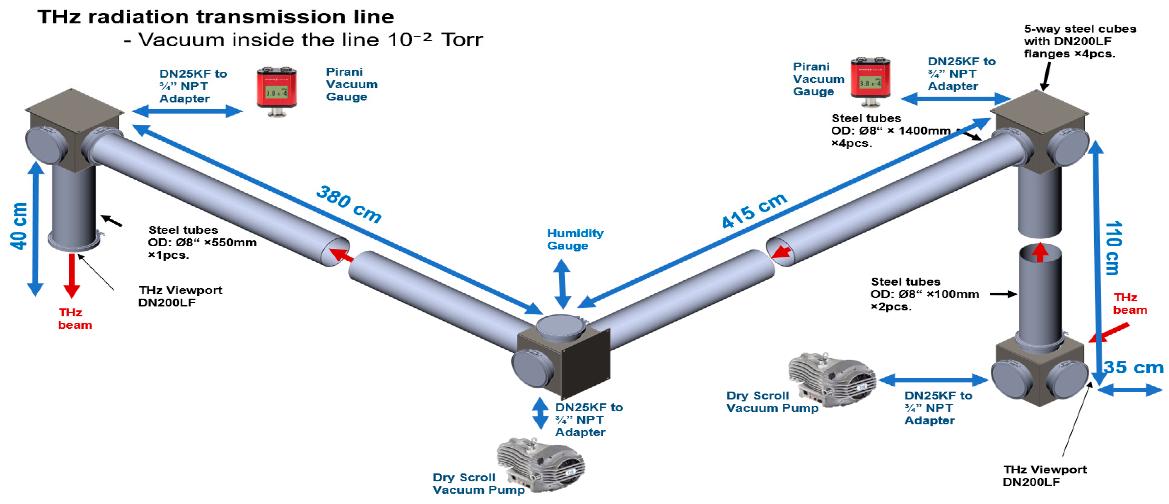
Figure 1 shows a general scheme of the THz FEL. The frequency spread of the THz radiation is 10% around the resonant frequency. Due to safety restrictions, the THz radiation source is placed in an underground bunker. The TL passes the radiation to the users’ rooms, with the geometry determined by the constraints of the building structure designed before this research began. Due to the high absorption of THz radiation by humidity in the air, the TL should be placed in a cylindrical plastic/metal pipe 30 cm in diameter under proper vacuum-enabling conditions to reduce losses, as shown in
Figure 2.
The TL consists of four sections perpendicular to each other. Confocal mirrors with a 90° reflection angle are installed at each junction of the central ray. Therefore, all mirrors have a common focal plane. Mirror no. 3 is not typical (even among mirrors with defined geometry, such as parabolic, spherical, etc.) in terms of the focal length. That is why its price is extremely high. This is the reason why many studies are now conducted on this topic, particularly with an emphasis on mirrors for THz. Another reason is that real radiation has a very broad spectrum. Specifics of the signals, such as an energy spectral density distribution (dW/df) of the complex beam is shown in
Figure 3, explained in detail in
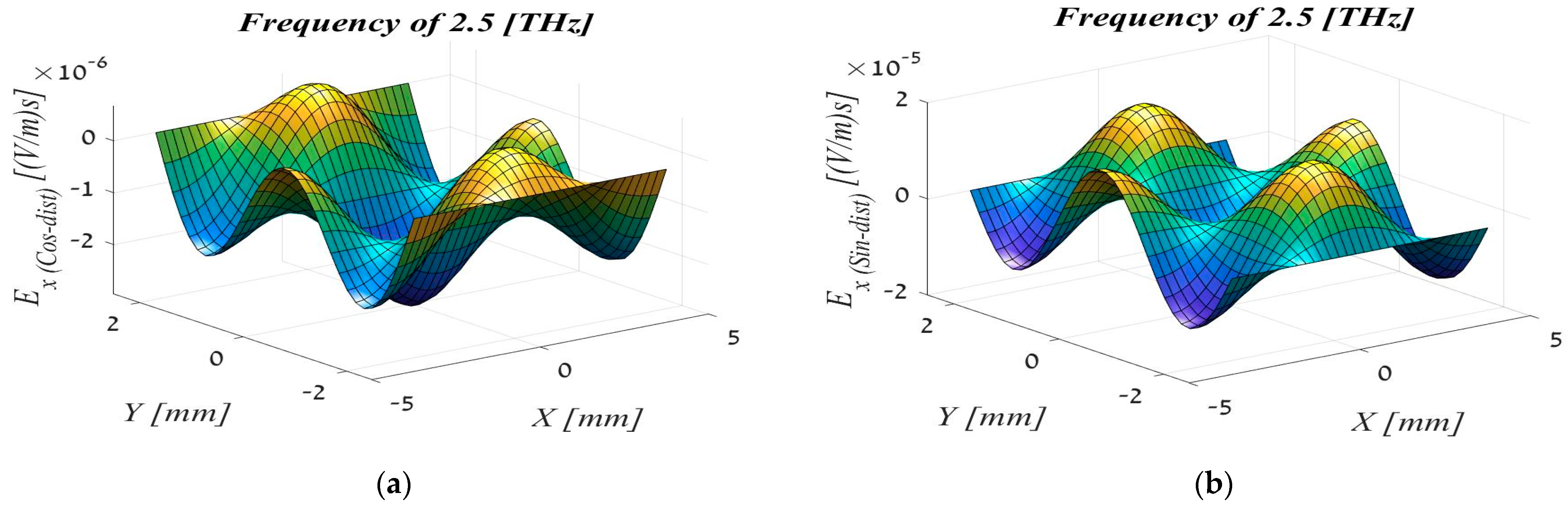
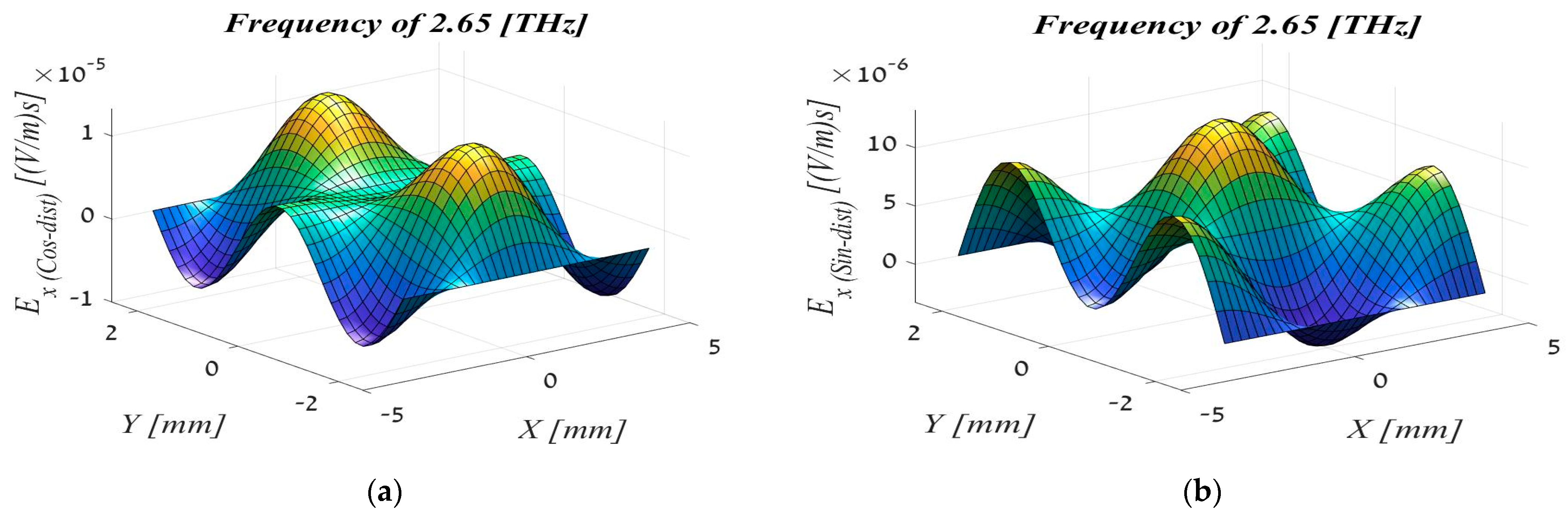
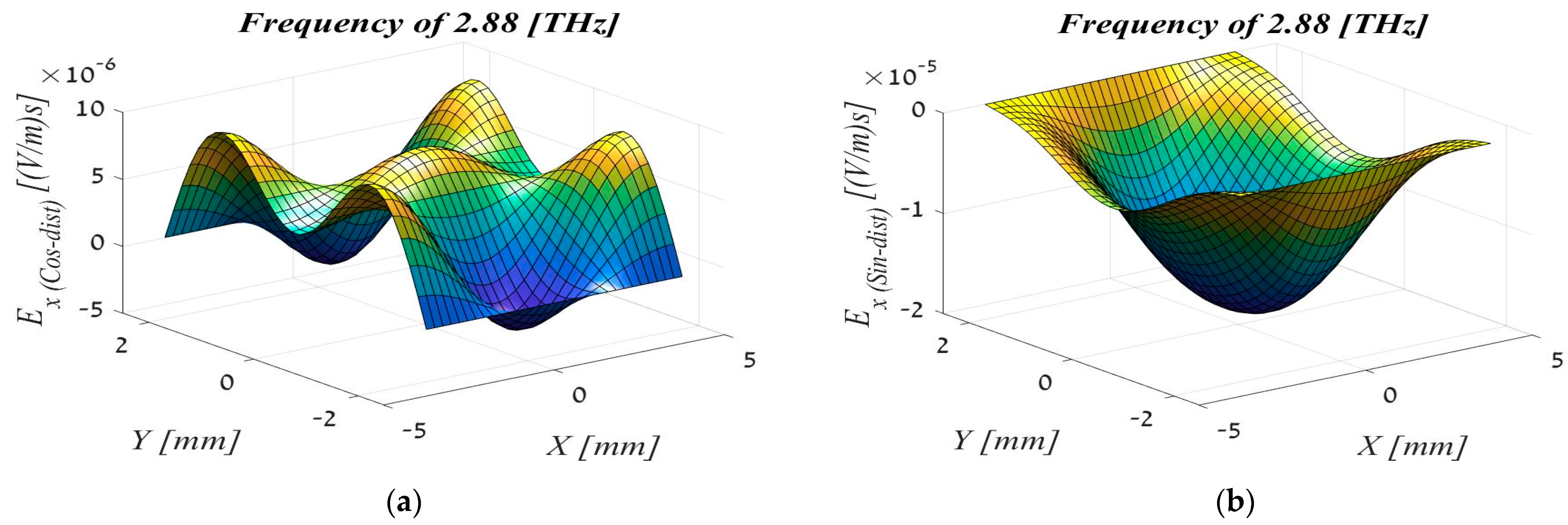
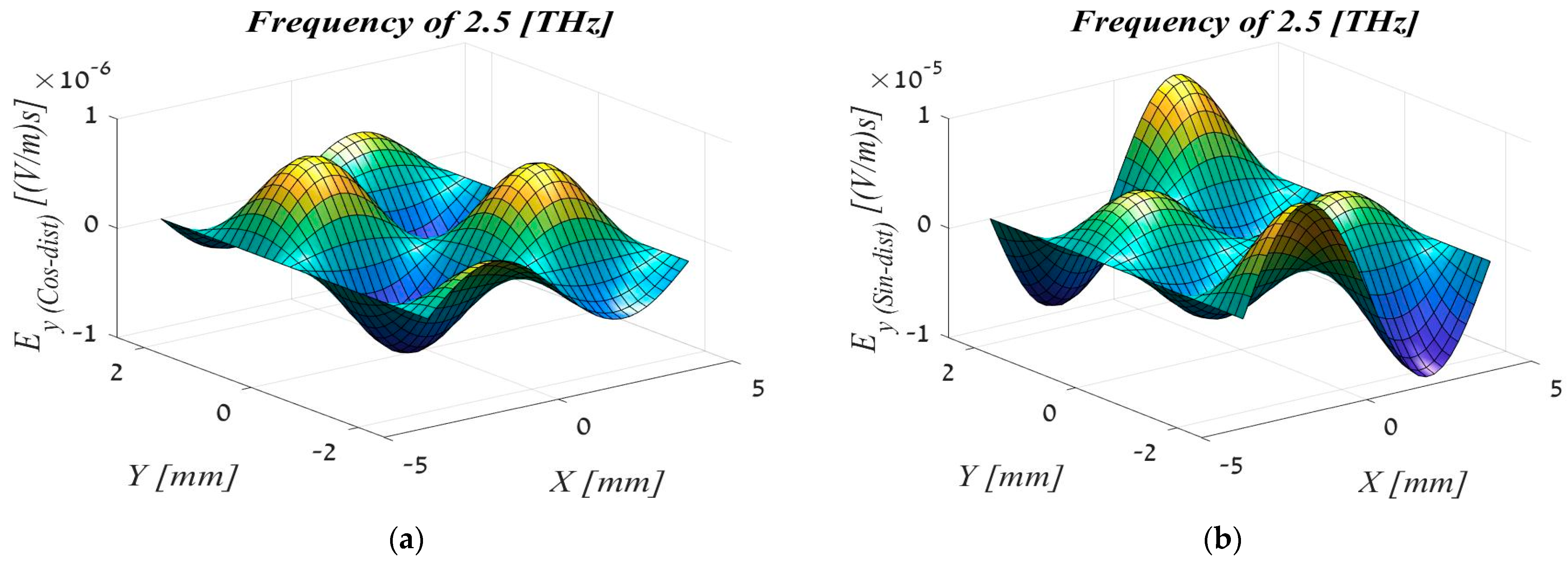
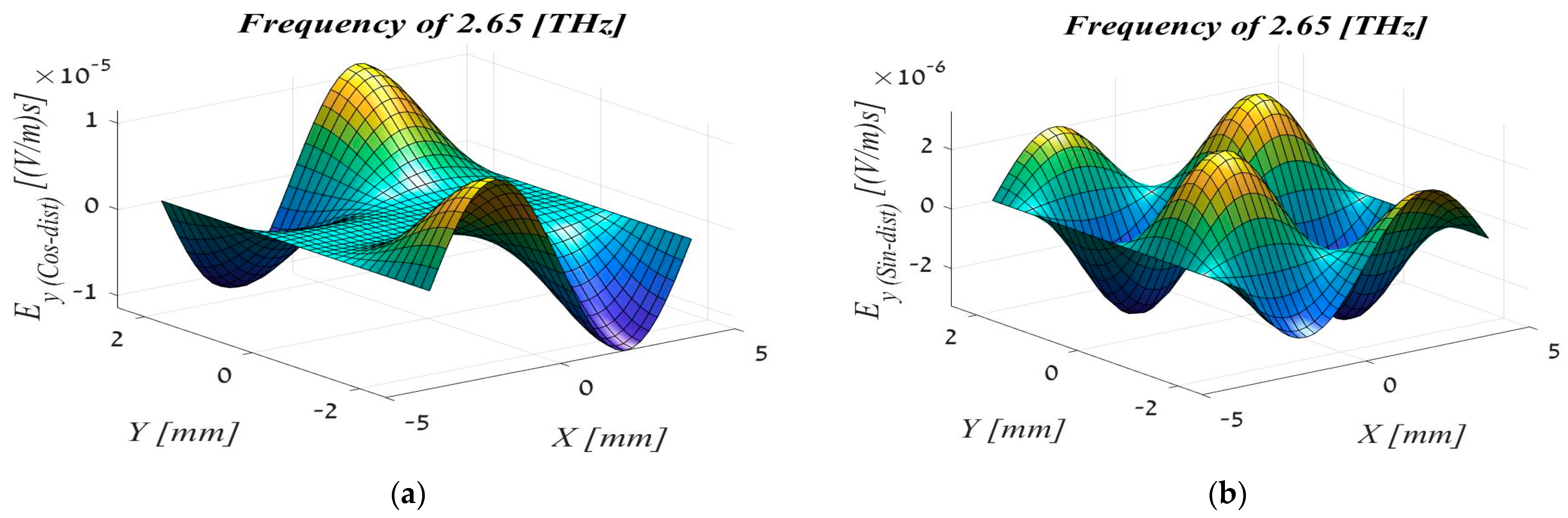
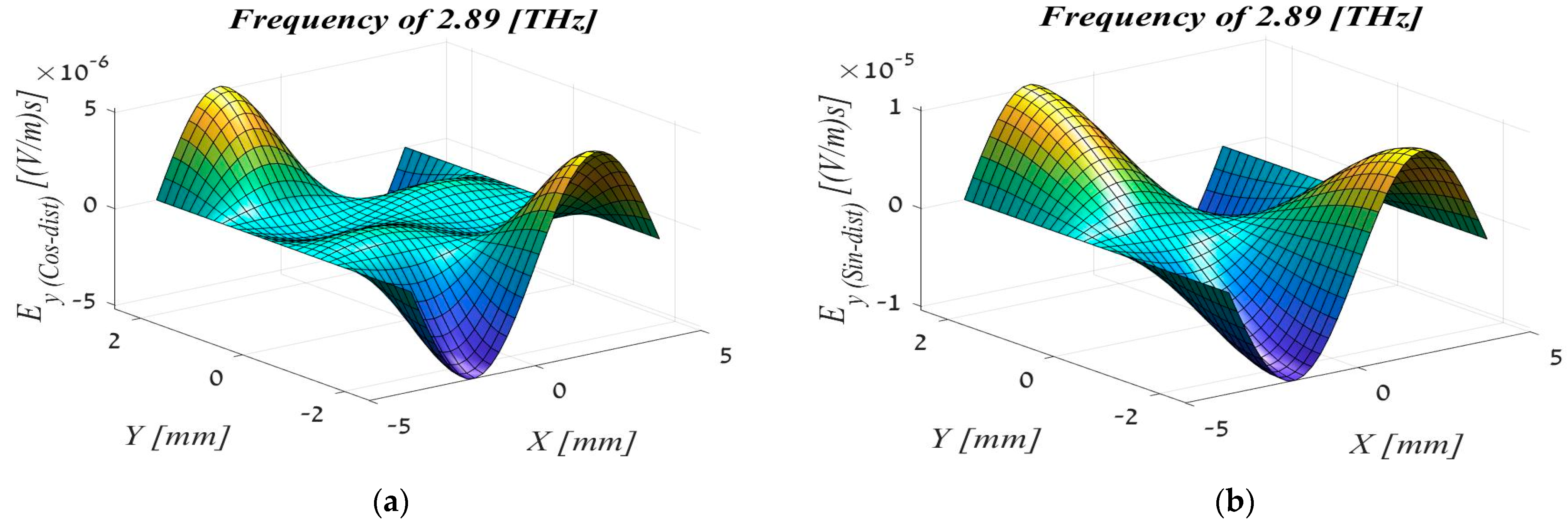
Section 3. In addition, we are planning for an FEL system that will work in the 1–4 THz frequency range. Even in such a medium, the properties of the radiation change significantly, with an emphasis on diffraction. (Without going into detail, it is worth noting that first, energy at a frequency of 1 THz will be lost on the sides in this configuration, thus there is a need for mirrors with a larger diameter.) This means that even for the same pulse, different TLs with different parameters are needed because the shape of each beam will change drastically, even at near frequencies, as shown in
Figure 4,
Figure 5,
Figure 6,
Figure 7,
Figure 8 and
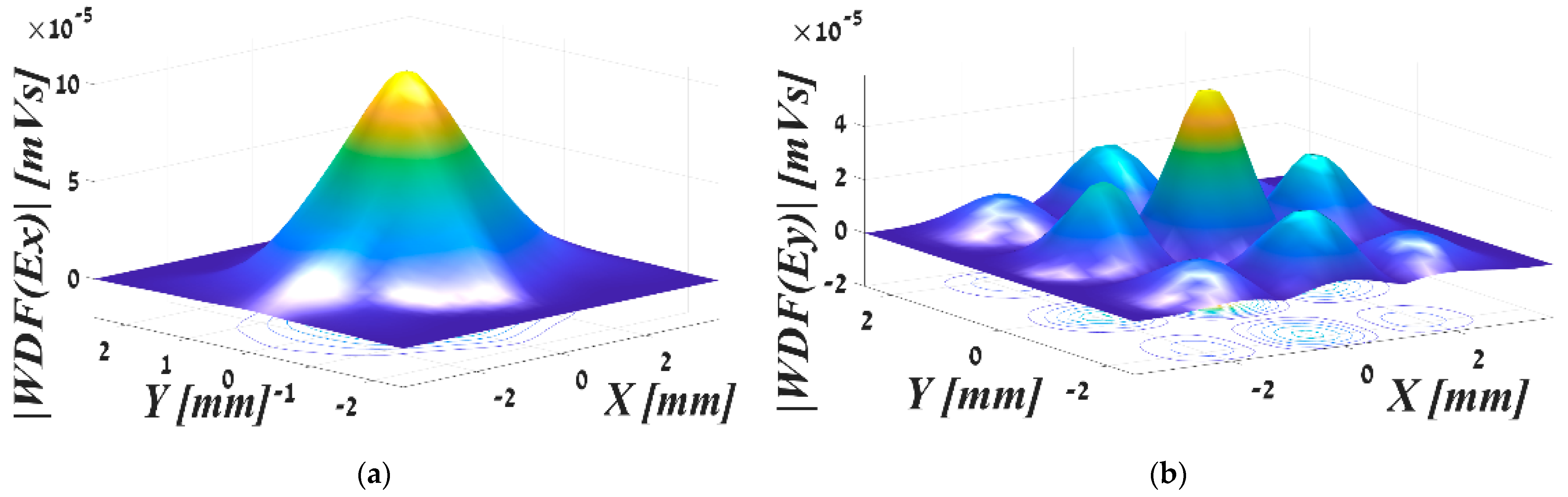
Figure 9. In addition, even at the same frequency, the shape of the Ex beam (
Figure 10a) is completely different from that of the Ey beam (
Figure 10b). This means that the energy distribution is completely different, which presents challenges for the entire TL in general and the mirrors in particular. Therefore, according to the initial estimates, it is clear that there is a need for different mirrors for 1 THz and 4 THz. It should be emphasized that, even for the same profile (pulse shape), different TLs with different parameters are needed. In order to accurately plan the mirrors, it is necessary to perform a calculation for the entire shape of the pulse and match it with a mirror. Then, we can optimize the mirror for a variety of radiation profiles. The components of the fields used for this purpose are shown in
Figure 4,
Figure 5,
Figure 6,
Figure 7,
Figure 8 and
Figure 9.
By default, Gaussian pulses are considered in most cases. Such a profile or shape is very convenient for scientists for a number of well-known reasons. It is also easy to follow the propagation of these pulses as well as how they spread or expand. The Gaussian pulse, or one with a similar normal distribution, correlates well with mirrors with mathematical geometry, such as parabola, ellipse, and spheroid. A certain caustic is created around the focus point, which makes it easy and convenient to calculate and work with. In practice, the pulses are not Gaussian at all [
13]. Therefore, there is a need to accurately characterize the beam in order to design the appropriate mirrors for maximum energy transfer. This is the main reason why we need to analyze and characterize the radiation. Additional support will be provided showing that the simulations are necessary for the further design of the TL.
The basic TL consists of two pairs of mirrors: a telescopic pair and a microscopic pair. There are other elements that are less important to this work. The scattering of the THz beam is quite large in relation to the visible light rays and the laser beam. It depends on the frequency (mode number and initial aperture distribution), but let us assume that its waist doubles every several inches [
14]. Therefore, it is necessary to focus on each beam at the beginning of the TL. This is the role of the first mirror. That is why the shape of the beam is extremely important (and the visualization in 3D). Another reason is that the general research (including research in various departments) deals with the construction of a smart TL using an AI approach, which learns the range of pulses and optimizes the mirrors for the purpose of transmitting radiation most efficiently at the main working frequency for the transmission of optimal radiation at a variety of frequencies. This work instead deals with characterizing the energy distribution for the purpose of general study.
The previous TL design was based on parabolic mirrors, considering solely the Ex part of the E(Ex, Ey) complex EM field. Ex itself is a complex beam transmitted as an ultra-narrow pulse, which is a rather complicated matter because the beams (real and imaginary parts of Ex) also change over time. Therefore, the design was performed according to the absolute value of the Ex complex beam when it is at maximum amplitude. This function is approximately reminiscent of a particular Gaussian beam (
Figure 10a). Therefore, parabolic mirrors were chosen. This is how the TL is actually planned and built in most cases. This approach allows for precise planning, considering all the parameters. In addition, for the first time, a complex Ey beam was explored as a preliminary result specifically for this work, while the emphasis in this study is on the 3D characterization of the entire EM field and analyzing all of its components separately.
As long as the accelerator is under construction and the TL is in the design stage, it is not possible to conduct experiments, so this is another reason for developing a quality simulation. Experiments can be carried out in similar systems for the purpose of justifying a later method, such as a diagnostic method for THz pulses produced by EA-FEL [
13].
2. The Gap and General Approach
2.1. Review of Simulation Methods
The Wigner distribution function (WDF) is one of the methods used for analyzing radiation and its propagation, which not many researchers commonly use, as few of them know it well. Most researchers prefer classical methods, such as solving the Maxwell equation with various computational accelerations. This requires them to reduce the resolution due to an endless demand for resources such as memory and computing power. Most physicists see problems in the techniques they have learned, and as a solution, they approach ready-made “solvers” in the hope that they will give them the best answer. This is understandable because they do not have engineering evidence and algorithmic tools. Therefore, in order to solve complicated numerical problems, commercial software is used, such as CST, HFSS, FDTD, and Zemax (Zx), even when these methods provide a limited solution and do not meet all the parameters. For this type of problem, CST is not effective at all; it has no built-in solvers and is simply not designed for this type of task. Except for Zx, these electrodynamic solvers require that the boundary conditions be defined. In fact, their solution is aimed at modeling compact structures that have an energy flow in arbitrary directions of the Maxwell equations. Due to the short wavelength, the grids become prohibitively large and require extensive power and memory. Each dimension requires at least 10 space samples per wavelength. Concretely, the space mesh cell size (∆r) is about 10 µm. The ratio of time-step size (∆t) correlated with the space mesh cell size has the relationship ∆r >> C0∆t, where C0 is the speed of light in a vacuum. Thus, such a solution requires about 1017 space mesh points and 106 time steps for each EM field component. Hence, FDTD functions quickly in the THz area. In addition, a large number of mesh elements and samples must be used, which increases the accumulated computation errors.
Zx is suitable but with strict restrictions, and the input data must be in the form of GO rays, which was the case in this work, and when we already have the EM field representation in the rays, then Zx is no longer useful. In addition, in order to set lenses or mirrors, the dimensions of Gaussian parameters such as maximal angle must be supplied. This is repeatedly an approximation to a Gaussian beam. The effect of each mode on the TL was calculated separately and analyzed and representation in Zx was carried out in [
14]. Working with Zx is very complicated and always requires a researcher familiar with it. In addition, there is a constant need to be in touch with technical support. Besides the limitations of the software, dedicated requirements, and approximations of the data, the license is very expensive, and this is why our center and all of the universities in our country have stopped working with it. Therefore, in this study, all the simulations (and their algorithms) were designed from scratch. The pulses are at the THz frequency, which requires enormous resources, and therefore, the known methods and techniques that were not suitable for this work were rejected, including the techniques discussed in [
15]. In our previous work, the TL was investigated with Hermit Gaussian (HG) modes [
16]. The study was performed by estimating the important parameters of the TL and the radiation that emerges in users’ rooms [
17]. This was a fairly thorough study, under limitations that we overcame in the present work. In the previous work, spacial profiles of the output radiation field components with the same characteristic frequency points were considered only for the Ex beam module. Also, the TL model was simplified to the on-axis and central axis when the mirrors were approximated with thin lenses. The most important factor was that the previous work used Gaussian beam mode analysis to describe the propagation of the wave packet emitted from the waveguide. The evolution of the Gaussian beam parameters in free space and the optical elements were described by using ABCD matrices [
18]. Implementing this technique in c++ code enabled us to demonstrate the energy distribution pattern of a multi-mode EM beam in different transverse planes along the TL. This has a great significance in the design of optical elements along the TL (by fitting them with dimensions corresponding to the EM beam), and understanding the consequences of the TL diameter on the energy loss pursuant to beam divergence. Using the methods considered and implemented in this research, the field pattern and beam width in front of the optical elements along the TL were estimated, as well as the energy flux distribution spectrum for the wave packet under concern and the TL. Actually, this is a favorite numerical calculation method among many researchers [
19]. The method is quite convenient but fixed in hard limits under non-negligible approximations. It must be noted that the most prominent disadvantage here is that the method works only for paraxial approximation for very small angles. An important conclusion was obtained from this research, which reinforces the use of the method proposed in the current work.
Most studies that use the WDF emphasize field representation in the time–frequency domain (of transformation), whereas in this study the emphasis is on the spatial–frequency (phase space) domain, with time–frequency as an additional option in order to estimate the field expansion in space. In addition, most studies address one dimension of the WDF, probably due to its complexity. In this study, we present a 3D analysis of the space–frequency and time–frequency domains.
In addition, as already mentioned, this work constitutes a basis for calculating radiation transfer in the most efficient way in future research when the planning techniques applied are ML methods. In other words, some non-trivial pulses should be transmitted in the most efficient way through the TL. That means, without changing the pulse and losing its power (energy), the medium should be changed in such a way that allows the pulse to pass in the most efficient manner. It is clear that each pulse will require a different change of medium; therefore, there will be some optimization of the range of pulses and frequencies. The second goal is to perform the field transformation from the shape of some function to the desired Gaussian. That is, it is a mode conversion. Therefore, the classical and other known methods cannot provide any answer to our challenge. Hence, the WDF was chosen.
2.2. Research Purpose
In addition to what was mentioned earlier, the technical aspects are emphasized here. The goal was to characterize the radiation profile of wideband ultra-short THz beams. As stated, each component of the EM field (Ex and Ey) is complex. Therefore, the pulse will be represented by four components (real and image amplitude for Ex and Ey, respectively) for each individual frequency. This is intended for future calculation of the smart mirrors that will transmit the pulse most effectively. This simulation is an integral part of the overall system design. Assume that the beam is pure Gaussian. Therefore, a mirror (let us say the first one in the current TL) that has a suitably defined geometry (as mentioned in the Introduction) will focus the beam in a certain caustic around the focal point. Even without going into non-linear effects, such as aberrations (for which a pair of confocal parabolic mirrors cancel the second order, and we have exactly two such pairs), under conditions of perfect geometry, when the beam is also defined in a precise mathematical way, the TL can be studied by HG modes [
17]. Indeed, mathematical answers that line up nicely are achieved for the planning of the TL in general and mirrors in particular. This is a classic method, well accepted in the field, which we have carried out this research [
17].
Obviously, HG decomposition is an approximation, if at all possible, and therefore it introduces an additional error when unsatisfactory results are obtained under ideal conditions, and all this is under paraxial approximation only. This approximation was made for a real part of the Ex field only, or its modulus. In reality, the beams are not Gaussian. The profiles are completely different from pulse to pulse, even for the same field at the same frequency at the same time (the Ex beam is completely different from the Ey beam), as shown in
Figure 3,
Figure 4,
Figure 5,
Figure 6,
Figure 7,
Figure 8 and
Figure 9, and even their absolute value (
Figure 10), the shapes of the pulses, that is to say, the profile functions, are not completely Gaussian. Therefore, the most appropriate method in this case is the WDF. The beam’s components are orthogonal and therefore can be separated for calculation. As noted in the Introduction, THz radiation has properties of both millimeter waves and visible light. Therefore, diffraction is very high, and it is necessary to focus the beam along the TL trajectory. The WDF allows the field to be represented as a set of GO rays when diffraction is considered. It can be seen that the EM field transmission by the GO rays leads to excellent results for frequencies 10 and 100 times lower [
20] (also published as GJM [
21]), which are known to have significantly higher diffraction than in this study. In addition, this experimental study shows that it is possible to reduce the scale and work with a small model of the tunnels. The results show excellent correlation both with the scaling change and in comparing simulations with real experiments in tunnels. In fact, this exactly fits the design of the TL. The mirror design was explained to justify this work as a simulation for a general purpose.
The main goal was to design a TL to transfer radiation in the most efficient way. Hence, the shape of the mirror and its profile function must also change according to the functional components of the beam. This work provides a spectral analysis of all components of the field, for each frequency and mode that make up the beam. Another advantage of this work is that all of the parameters can be changed, so this simulation is a broad platform for the analysis, characterization, and diagnostics of radiation. At the same time, an LF is obtained, which can form the basis of input data for work with the RT technique in any software, input data for AI systems, or input data in Zx format or other commercial simulations in optics and quasi-optics. This is another reason for choosing the WDF.
4. Methodology
The WDF has long taken pride of place in the field of optics [
25] and quasi-optics. It was introduced by Eugene Wigner in 1932 as a quasi-probability distribution to study quantum corrections to classical statistical mechanics [
26]. The WDF plays an important role in the characterization and propagation of electromagnetic fields and is a tool for modeling optical field (linear and nonlinear beam) propagation [
27]. One can see from previous publications that the analysis works for both coherent and partially coherent beams. Thus, there are current publications on this topic regarding both the paraxial and non-paraxial regimes [
28].
In addition, it has become a very useful tool for the theoretical analysis of optical (including quasi-optical) systems [
29,
30], acoustic holography [
31], signal processing [
32], radar emission [
33] for its characteristic representation, and radio waves used in wireless technology [
34]. It has been utilized in numerous applications as well as real physical experimentation. The WDF is related to time–frequency analysis [
35] in a vast majority of studies and is less applied to spatial frequencies, which are of greater importance in this work.
A general approach to complex electromagnetic (EM) fields is represented in this research, where each beam component, such as Ex and Ey fields, is also complex. In addition, the novelty here is an inexact description of free electromagnetic wave fields in terms of rays [
36,
37] with emphasis on THz radiation systems and spectroscopy (see [
15,
38] and references therein).
The WDF is a new way of characterizing EM fields, especially as a unified description of partially coherent beams when exploring the concept of phase space. Following Alieva et al. [
39,
40], evaluation intensity, phase coherence, beam width, and other beam parameters during propagation can be described by the pure space or the pure spatial–frequency representation of a stochastic process via its mutual intensity (MI).
MI is a function of four variables in Equation (1), where r1 and r2 are vectors. It describes the beam behavior, where the brackets are used for time or spatial averaging and the asterisk (*) indicates a complex conjugate. The intensity distribution I(r) corresponds to a square module in Equation (2). This parameter can be measured.
The WDF of an EM field,
, is defined by its MI, represented in Equation (1). It can also be described in terms of its directional spectrum, as represented by Equation (2) and its equals (according to [
39,
40]).
Therefore, it is easy to explain the “ray concept” in the GO by this space–frequency description. In ray optics, each ray is defined by its position and direction. Hence, the WDF of each beam,
W(
r,
p), is the amplitude (3, 4) where the ray passes through point
r with frequency
p (i.e., direction q).
A set of GO rays defined by the WDF represents the EM beam propagation in space [
41]. Let us define a flat aperture as the initial position of that ray’s set; in the real world, this flat aperture is the waveguide’s output. The WDF of the beam is perpendicular to the
z-axis in an ideal case. To simplify the explanation, let us concentrate on a known monochromatic field distribution on the aperture. In this simple case, the WDF of a total complex E(Ex, Ey) field in terms of rays can be defined for each component separately, and this also helps to simplify the task because the Ex complex field is orthogonal to Ey.
Therefore, the WDF of the Ex can be defined as follows:
The WDF of the Ey can be defined as follows:
Coordinates (x, y) are the physical points on the aperture (waveguide output). The space angles () are conjugated variables of a Fourier transform in the space coordinates. When the time dependence of the EM field transfers is considered, the dimension of the WDF increases from 4D to 6D.
As a result, the rays from each point
xy on the aperture are obtained. The direction of each ray is defined by the wave number
, where
The complex ray amplitude and polarization (I) are defined by the WDF as
The complex ray amplitude
is obtained due to the orthogonality in any uniform media of the ray polarization to the ray wavenumber (
).
Thus, for each given beam distribution (E), the set of rays I
) is obtained for each physical point (
x,
y) on the aperture. The Ex and Ey beam propagation in space is represented by the propagation of the GO rays [
41]. All equations represent a single-frequency problem. For multiple-frequency problems, we follow all steps mentioned above for each frequency separately.
5. Results
WDF Simulations
The vast majority of studies that use the WDF focus on its time domain is 1D. In this study, the 3D spatial domain is important in order to diagnose the form of energy distribution for each beam, as well as the beam’s propagation. Almost all researchers have used the WDF for analytical solutions. However, no simulation was found for our needs. Therefore, a special code to implement the WDF was developed from scratch for this study purpose. For each coordinate in space an LF is obtained, a pulse consisting of rays at all kinds of angles. The number of rays and representation of angles can be controlled according to the need and convenience, depending on the resolution of the aperture (which depends on the initial sampling resolution).
As can be seen from Equations (5) and (6), for a simple two-dimensional field, a 4D WDF is obtained. The complex amplitude adds an additional dimension. The XY physical coordinates mark the initial beam position on the aperture. Kx and Ky are spatial angles relative to the
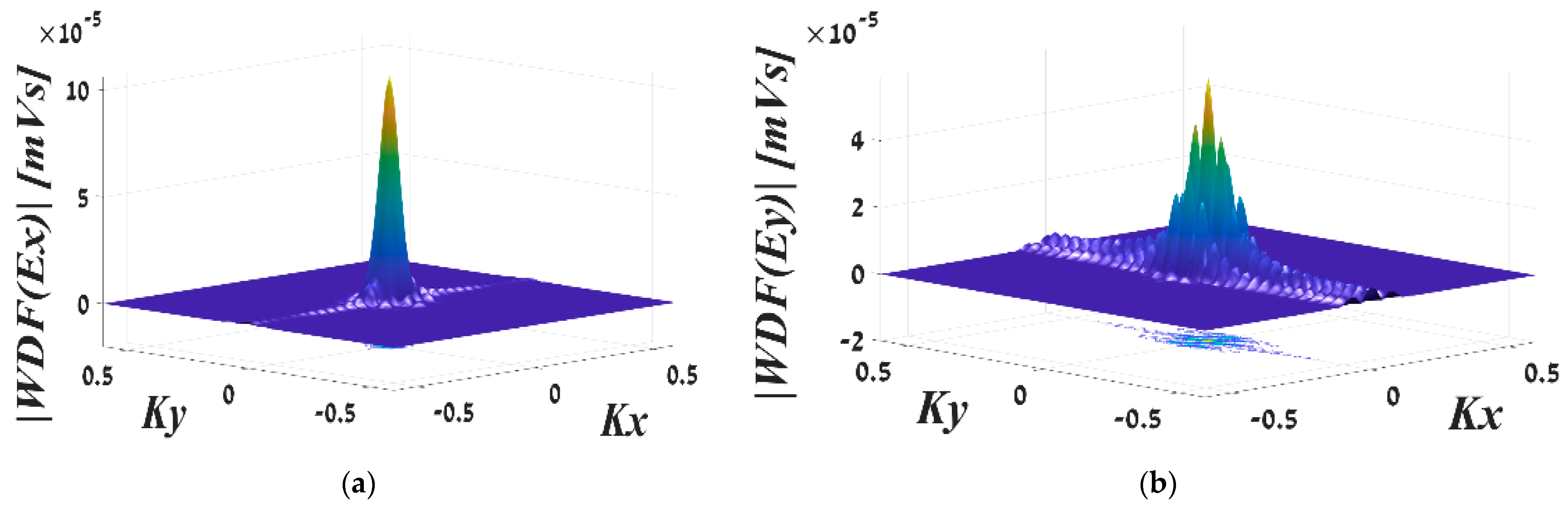
Z-axis. The beam is not static and it changes over time; therefore, another dimension is added. These changes are harmonic and behave according to sine and cosine. The LF in the center of the aperture (coordinates X = 0 and Y = 0) is shown in
Figure 11.
Figure 11a shows the WDF from the Ex beam and
Figure 11b shows the WDF of the Ey beam. The figure shows the total of rays in all directions emerging from the midpoint (center) of the waveguide. In Ix, the angle spread of K
x and K
y is very small and thus is negligible in the energy dispersion. It can be concluded that the radiation is focused and directed exactly parallel to the
Z-axis, without unnecessary deviations, and the energy is mostly concentrated in the center. In the Ex beam, the first mode is dominant, thus the shape of the field is reminiscent of the normal distribution in the middle. When most of the intensity is concentrated in the middle of the field it is uniform, thus in the representation of the rays, a uniform concentration is also seen in the middle. Therefore, paraxial approximation can work in this case and can indeed be simplified with Gaussian beams.
Figure 11b shows the Ey field representation, where 12 concentrations of different transmission angles can be seen. These are the most important 12 directions, but their scattering is not large and is concentrated around zero. That is, the significant transmission direction is parallel to the
Z-axis. This is because the energetic distribution of the Ey beam is uneven on the aperture, consisting of four peaks. It can be concluded that the dominant mode at the resonant frequency is mode TE
21.
A type of ripple can also be noticed. In
Figure 11a, the ripple is almost negligible, which means that from the center point, there is almost no transmission of rays at large angles relative to the
Z-axis. In
Figure 11b, a more significant ripple can be found, which indicates that there is energy at the edges. But here, too, the transmission concentration is along the
Z-axis. This is less important in this study, but what stands out is the direction of the ripple. In
Figure 11a, it is along the
X-axis, while in
Figure 11b it is along the
Y-axis, which reinforces the correctness of the result obtained. The directions of the ripple vary with respect to the direction from which it reached the center of the aperture, but what is saved is the attitude. The ripple that appears in Ix is perpendicular to the ripple in Iy.
Figure 12 shows the entire aperture containing all the rays emanating parallel to the
Z-axis from each defined coordinate (Kx = 0, Ky = 0). It is worth noting that these rays have the highest intensity because of the original transmission direction along the
Z-axis. Therefore, it can be seen that almost all the energy is concentrated in these rays.
Figure 12a shows the normal distribution reminiscent of Gaussian, which makes sense considering the shape of the Ex field. This is further confirmation that a paraxial approximation can work in this case and it is indeed possible to simplify with Gaussian beams.
Figure 12b shows the special and non-uniform distribution. It is found that the rays emitted parallel to the
Z-axis do not constitute a uniform energy distribution. These are eight main equal distributions, with the main transmission direction being along the
Z-axis. In addition, we can see the level in the middle, which indicates the level of radiation at Kx, Ky = 0.
In fact, this is the most significant information describing the behavior of the beam for the purpose of this study.
6. Discussion
This work presents the spatial profile of output radiation for a complex EM field, where all of its components are complex beams and the entire beam component is transmitted as an ultra-narrow pulse. The results were obtained as expected and with the desired resolution. It is worth noting that
Figure 10,
Figure 11 and
Figure 12 were constructed after interpolating the representation in Matlab for better understanding.
Figure 12a shows the normal distribution reminiscent of Gaussian. As mentioned, the propagation direction is along the
Z-axis. Therefore, the pulse that advances parallel to the
Z-axis behaves like a Gaussian beam and carries most of the energy. Therefore, if only parallel rays were translated, this would mean the transmission direction is precisely aimed, and there would be no need for a smart mirror. Also, the initial design of the TL with parabolic mirrors is quite correct. But the wisdom is to transmit the radiation in the most efficient way. It can be concluded that this is the desired distribution in the final stage of the target.
It can be seen that the intensity of these rays is also very high compared to the rays that are emitted in different directions relative to the Z-axis. It can be clearly seen that the larger the angle of the Z-axis, the lower the intensity. This is consistent with the theory and is pointing such that most of the radiation will propagate parallel to the Z-axis, as planned.
Figure 12b shows Iy. At first glance, it might seem that something here is not understood. When representing the intensity of the Ey beam in
Figure 10b, there is no amplitude in the middle of the aperture, whereas
Figure 12b shows all the rays that were emitted in parallel from the entire aperture space. A logical question arises as to where the radiation came from or whether something is wrong with the simulator.
In each case, we tackled the problem, despite the challenging obstacles. Finally, the strongest radiation was received in the center, as shown in
Figure 12b. Therefore, we performed an integration of the central point and its environment; when the integrated information is taken, it is full of complexity. The result, according to an accurate calculation, is Iy (0, 0) = 5.6404e − 23 + 5.0770e − 23i. It can be assumed that the answer is zero. Applying the WDF to the actual and simulated parts separately also provides a nil result.
Yet the result shown in
Figure 12b is correct, as the representation, in the sense of the rays through the WDF, shows the phase space. In other words, it presents the spatial frequencies, and spatial distribution is represented here, as mentioned. This means that the phase, angle Kx, Ky = 0, shows us the spatial frequency 0,0. Looking at
Figure 10b, we see the positive peaks around zero. We can imagine an absolute sine signal or the square of a sine (in a single cycle window). After a one-dimensional Fourier transform, with the harmonics of sine, positive and negative plus zero frequencies are obtained. This means that DC is calculated as the average of the signal. This is exactly what is seen here, just in 3D. We find that the WDF is productive on MI, as can be seen from Equations (3)–(6). This is not so trivial, especially at first glance, therefore we will explain it here.
As mentioned in the analysis of the results,
Figure 11a shows the intensity of the radiation of the Ex beam, while
Figure 11b shows the intensity of the Ey beam. This provides an excellent indication that the radiation is mostly advancing parallel to the
Z-axis. At the same time, it is known that the WDF maintains the profile of the real beam. Therefore, when such an indication is found in the sense of the rays in terms of spatial frequencies, it can be concluded that at a frequency of 2.889 THz, there is synchronization between the electronic beams and the undulator. Further analysis of the subject goes beyond this framework and is within the purview of researchers from another department. As also mentioned with respect to the ripple, it is perpendicular between Ix and Iy (
Figure 11a vs.
11b). Because the simulator computes the beams, the desired and expected result was obtained. We can see that the absolute value of the Ey beam is indeed perpendicular to the absolute value of the Ex beam in all the images, especially their absolute values, as shown in
Figure 10.
Figure 12a clearly shows that the HG mode decomposition method is not suitable for this design. More precisely, we can actually see the condition for using HG, that is, provided that the angles are very small, a paraxial approximation, as claimed in the Introduction. We have received support and justification for the WDF method, which is also shown here by the fact that in a paraxial approximation, a beam behaves approximately as a Gaussian. The exact same distribution is shown for the Ey beam in
Figure 12b.
7. Conclusions
This study presents the 3D spatial profile of output radiation for non-trivial radiation, transmitted as an ultra-narrow THz pulse for the design of a TL of an innovative particle accelerator. From
Figure 12 it can be concluded that a parabolic mirror, positioned parallel to the propagation axis, is approximately suitable for transferring most of the energy.
In this research, a special tool was built to handle that challenge. A unique simulator was built from scratch. The simulation provides the ability to perform 3D diagnostics for an early TL design by analyzing such special radiation. The radiation characterization can be achieved from 3D imaging of the ultra-short THz pulses and its visualization. A mirror design as part of the TL can be calculated from the LF [
42], as a representation of the complex EM fields. The algorithm is adjusted for phase–amplitude and spectral characteristics of complex multimode radiation generation in a free-electron laser (FEL) operating under various operational parameters. A general EM field on the edge of the source is represented in the frequency domain in terms of cavity eigenmodes. This representation is the result of a WB3D simulation, developed to obtain an indication of the complex EM field.
A 3D space–frequency analysis was provided by the WDF to discover hidden details, in which a complex EM field is transformed into a set of geometrical optical rays. Such representation is much simpler to describe the dynamics of EM field evolution in future propagation analysis and allows us to determine an initial design for the TL. A general ray approach allows operation in linear and non-linear regimes [
27].
The simulation was successfully implemented for the purpose of calculating, analyzing, and 3D diagnosing special radiation with quite extreme parameters when the accelerator itself is challenging and the process is detailed so that it no longer matters what the frequency is or how short the pulse is, at least when working with simulations, until the technology allows to detect and visualize single extra-narrow pulses in the THz region. Among the recent progress made in the THz application using classic methods for computing EM wave problems is a transfer matrix method, which simulates some mediums and transmits the rays. Our simulation is a basis for using these methods, such as the RT method, Zemax, and others.
To sum up, we received a bonus, which was an ultra-short pulse simulation of THz, which we converted to a representation in an LF. Hence, all the techniques of geometrical optics are valid. From here, we can use all the techniques of image processing, data compression and coding of the integral imaging data [
43], computational imagingand parallel processing. The method is most convenient for parallel processing [
44] and can be run with a GPU.
The simulator was designed with Python code from scratch, without the use of built-in functions for the special purpose of the accelerator center. The entire tool showed the correct results. When the tester encounters a complex EM field in the THz range with complex components, each component of the beam is an ultra-narrow pulse on the order of femtoseconds. All components of the EM field were calculated on a small aperture of 7.5 by 5 mm, which is a waveguide output. The Ey field is generally thought of as a precursor, and for the first time, its full characterization in 3D was obtained in this study. The method was developed for the phase–amplitude and spectral characteristics of complex multimode radiation generation in a free-electron laser (FEL) operating under various operational parameters. The tool succeeds in diagnosing an early design of the TL of an innovative accelerator at the Schlesinger Family Center for Compact Accelerators, Radiation Sources, and Applications and can be applied to any type of TL. We are confident that our tool can present the 3D spatial profile of any kind of output radiation, represented in terms of GO rays or LF along with an in-depth 3D analysis, according to the needs of the study.


 ,
, 


