1. Introduction
In recent years, the lattice Boltzmann method (LBM) has been widely used for numerical simulation of different physical phenomena [
1,
2]. Unlike the conventional methods, which are based on discretization of the equations for macrovariables (density, velocity, energy, etc.), in the LBM, the systems of fully discrete kinetic equations (so-called lattice Boltzmann equations, LBEs) are considered.
Based on LBEs, the computational schemes deal with the intrinsic coupling of time and space steps. It leads to the fixed value of the Courant–Friedrichs–Lewi (CFL) number. For LBEs, the CFL number is equal to unity, and it is a constraint stated on the values of grid steps. It brings a limitation to the standard LBM, because it leads to the impossibility of using variable time and space steps. This problem is relevant, for example, for the simulation of gas flows, where shock and rarefication waves take place [
3]. Such phenomena can lead to the necessity of the application of unstructured and adaptive grids and variable time steps. To overcome this problem, so-called off-lattice schemes, which are constructed using finite-difference [
4], finite-volume [
5] and finite-element [
6] methods, are proposed. These approaches are based on the independent discretization of continuous kinetic equations with discrete velocities on time and space variables.
Most existing schemes, based on LBEs, are restricted to weakly compressible simulations. However, for highly compressible flows, such schemes lead to some difficulties. One of the main reasons is that the equilibrium distribution functions used in the standard LBM are derived from the truncated Taylor expansions of Maxwellian distributions with the assumption of a low or moderate Mach number.
The straightforward extension of the LBM to the simulation of compressible flows can be achieved by increasing the number of discrete velocities and using appropriate equilibrium distributions. This leads to the commonly known multi-speed models [
7]. The standard approach for LBEs, based on collide-and-stream techniques, is less computationally expensive than off-lattice schemes. However, its application to multi-speed lattices leads to numerical instabilities [
8]. To avoid this problem, for many multi-speed models, the off-lattice approach is used [
9,
10].
Different compressible models are constructed for the opportunities to vary specific heat ratio, and Mach and Prandtl numbers. For the case of the fixed specific heat ratio, Yan et al. [
11] proposed a compressible model with more than one rest energy level. In [
12], the LB model for the compressible Navier–Stokes system with an adjustable specific heat ratio is constructed by adding a new molecular velocity. Watari [
13] constructs the kinetic equations with discrete velocities and additional degrees of freedom for 2D Navier–Stokes and 3D Euler models with flexible specific heat ratios and Prandtl numbers. Nie et al. [
14] propose an approach for treating the internal degrees of freedom of the polyatomic gas molecules. As it is mentioned above, traditional equilibrium distribution functions are based on the truncated Taylor expansion of the Maxwellian distribution, limited to low and moderate Mach number [
3]. Authors of [
15,
16] proposed the general approach equilibrium distribution functions constructing, based on the expansions on generalized Hermite polynomials presented in [
17]. Qu et al. [
18] obtained equilibrium distributions based on the circular function, which is not related to the Maxwellian distribution. In [
19], a general technique for the construction of equilibrium distributions for kinetic models of high-speed compressible flows is proposed. The approach is based on the solution of a linear algebraic system based on the equations for moments of distribution functions for the selected lattice and velocity set. In [
20], the control of the Prandtl number is realized by the modification of the collision term. In [
21], the multiple-relaxation-time scheme with a flexible value of this number is constructed. Zhang et al. [
22] tried to control the Prandtl number in the case of Burnett equations using an ellipsoidal statistical model.
Another class of discrete velocity models used for the computation of compressible flows is the double distribution function (DDF) models. In addition to a set of distribution functions for the computation of hydrodynamic variables (density, velocity), a set of functions for energy (or temperature) is introduced. One of the first models where functions for temperature are introduced is proposed in the paper of He et al. [
23]. Li et al. [
24] propose a coupled DDF-LB model for the compressible Navier–Stokes equations in order to achieve a flexible specific heat ratio. In [
25], this model is applied for the simulation of high-speed compressible viscous flows with a boundary layer. In [
26], this model is used for the simulation of shock wave propagation and its interactions with the boundary layer in a shock tube. As for the multi-speed models, in DDF models at high Mach numbers, the traditional collide-and-stream method, typical for the standard LBM, is not used due to the numerical instabilities (for example, see works [
27,
28,
29], where the off-lattice schemes are used). Saadat et al. [
30] propose a DDF model for the D2Q9 lattice with a correction of the collision term and a shifted lattice, proposed in [
31] for the simulation of flows with high Mach numbers. Qiu et al. [
32] constructed a DDF model based on the D2Q17 lattice for the simulation of viscous compressible flows.
In the literature, alternative approaches for compressible flow simulations, distinguished from multi-speed and DDF models, are used. The typical examples are the hybrid LBM, which uses both kinetic equations and equations for macrovariables [
33]; the pressure-based regularized LBM, which uses explicit correction terms for the pressure [
34]; hybrid recursive regularized versions of the LBM [
35,
36,
37]; and multiple-relaxation-time (MRT) models (e.g., see [
38]).
The presented paper is devoted to the analysis of discrete velocity models used in the LBM for the simulation of compressible flows and for construction of off-lattice computational schemes for practical simulations. In the theoretical aspect, attention is focused on the stability analysis of the solutions associated with the steady flow regimes. Multi-speed and DDF models, widely used in literature, are considered. The analysis is based on the stability criterion, related to the negativity of the real parts of the eigenvalues of matrices of systems, obtained after linearization of the governing equations and separation of variables. The stability domains in the parameter space are constructed and analyzed. It is demonstrated that some models can have larger stability domains than others. Selected multi-speed and DDF models in practice are compared on the numerical solutions of nonlinear problems, such as the Riemann problem and the Kelvin–Helmholtz instability (KHI) simulation. For the numerical solution, the parametric off-lattice finite-difference scheme is used. It is demonstrated that the numerical solutions obtained by different models are close to each other.
The following new results are obtained in the presented work:
1. The numerical procedure for stability analysis, based on the construction of stability domains in parametric space, is proposed.
2. The comparison of stability domains, constructed by the proposed procedure, is performed.
3. It is demonstrated that the value of the Prandtl number does not seriously affect the stability of DDF models.
4. The models are compared on the nonlinear problems of gas dynamics: Riemann problems and simulation of KHI. It is demonstrated that models lead to close numerical solutions.
The paper has the following structure.
Section 2 presents the discrete velocity models considered in the paper.
Section 3 is devoted to the stability analysis of the governing equations of these models. The approach of constructing stability domains in parametric space is proposed. The domains, constructed for different models, are compared.
Section 4 is devoted to the numerical experiments. A parametric off-lattice finite-difference scheme for the numerical simulations is proposed. Selected nonlinear problems in gas dynamics are solved numerically. Some concluding remarks are made in
Section 5.
3. Stability Analysis
Let the following dimensionless variables be introduced:
where
and
H are the typical values of
and
.
After the substitution of (
8) into (
4), the dimensionless system is obtained:
where
. The tilde sign will be ignored in the text below.
As in previous works (e.g., see [
8,
41]) the stability only on the initial conditions is investigated, so the flows in the unbouded domain are considered. The stability of the steady-state solutions of (
9), associated with the steady flow regimes, is analyzed. Let
correspond to the steady flow in the unbounded domain, defined by the constant values of dimensionless macrovariables:
,
and
. These solutions are derived from
, as
.
For the stability analysis of this steady flow regime, the solutions of (
9) are presented:
where
is a vector of small perturbations.
Let us consider the dynamics of
at
. For this purpose, (
10) is substituted into (
9):
According to the proposition on the small values of perturbations, the Taylor expansion can be used:
After the substitution of this expression into (
11), the following linearized system is obtained for the perturbations
:
where the components
are computed as
According to the Fourier method, the solutions of (
12) can be presented as follows:
where
and
is the wave vector,
. The structure of the solutions, defined by (
13), corresponds to the idea of separation of variables. After the substitution of (
13) into (
12), the following system is obtained for
:
where the components of
are written as follows:
For the model from [
19], the dimension of
is
; for the model from [
13], it is equal to
.
For the DDF models presented by system (
6)–(
7), the steady-state solutions, associated with the same steady flow regime, are computed as
,
. System (
6)–(
7) in dimensionless form is written as
,
,
.
The solution of (
15)–(
16) is presented in the same form as the previous case:
where it is proposed, that
,
.
The dynamics of perturbations
and
are described by the following system of differential equations:
where
The solution of this system can be presented as follows:
where functions
and
are the solutions of the following system:
where
If the extended vector
is introduced, this system can be rewritten as
where
By this approach, the problems of stability analysis of steady-state solutions are reduced to the problems of stability analysis of zero solutions of linear systems (
14) and (
17). These solutions are asymptotically stable if and only if the real parts of all eigenvalues of matrix
are negative. These eigenvalues are dependent on the following parameters:
,
,
,
,
,
and
(the models from [
24,
32] are analyzed at a fixed value of Prandtl number
, so only the value
can be varied if the value of
is inputted), where only the components of
are considered as the internal parameters. For the simplification of analysis, the values of two dimensionless macrovariables are fixed:
.
The stability is analyzed for the case of the following flow regime:
,
, as it is realized for other LB models [
41,
42]. The wave vector
can rotate relatively to
in all 2D space, as it is realized in [
8]. So, we restrict the parametric dependence of eigenvalues to the dependence of two internal parameters,
and
, and two input parameters
and
U. The values of
are chosen in small intervals near zero because the presented models in most problems are applied to the simulation of inviscid flows (when
). The values of
U are varied in a bounded interval including zero, in order to check the maximum value, which defines the stability interval on this parameter.
The stability is investigated by the construction and analysis of the stability domains in the 2D space of the input parameters . These domains are constructed by the following algorithm:
(1) The grids with nodes , , are constructed in the intervals , and rectangle , respectively. The values of T and are selected by the investigator.
(2) At every fixed node (
,
), the eigenvalue problems for matrix
are solved at every node
and eigenvalues
are obtained at every
p and
q. If at some node
the following inequality is realized:
, so the solutions of the systems (
14) or (
17) are treated as not asymptotically stable at
and
and node
is not included into the stability domain in parametric space.
The eigenvalue problems are solved numerically using the QR algorithm, realized on FORTRAN90 in EISPACK subroutines [
43]. We perform the computations for the monoatomic gas with 3 translational degrees of freedom per atom, which is typical for the air flow. For this physical condition, the value of
is equal to 5/3. The models presented in [
13,
19] are additionally dependent on the values of
[
13] and
,
. As it is mentioned in [
19,
44,
45], the value of this parameter can affect the numerical stability. So, we decided to investigate the influence of these parameters on the solutions. For the model from [
13] the values of
are chosen as
. It is inspired by the same approach of choosing
in numerical examples, presented in [
13]. In
Figure 2 and
Figure 3, the boundaries of the stability domains for different values of
are presented. As is demonstrated, for both models, the acceptable value of
can be chosen as
, and the greatest values of
U take place for the values
. As can be seen, the largest areas of the stability domains correspond to the model from [
13]. Moreover, its area does not change after the value
(see
Figure 3).
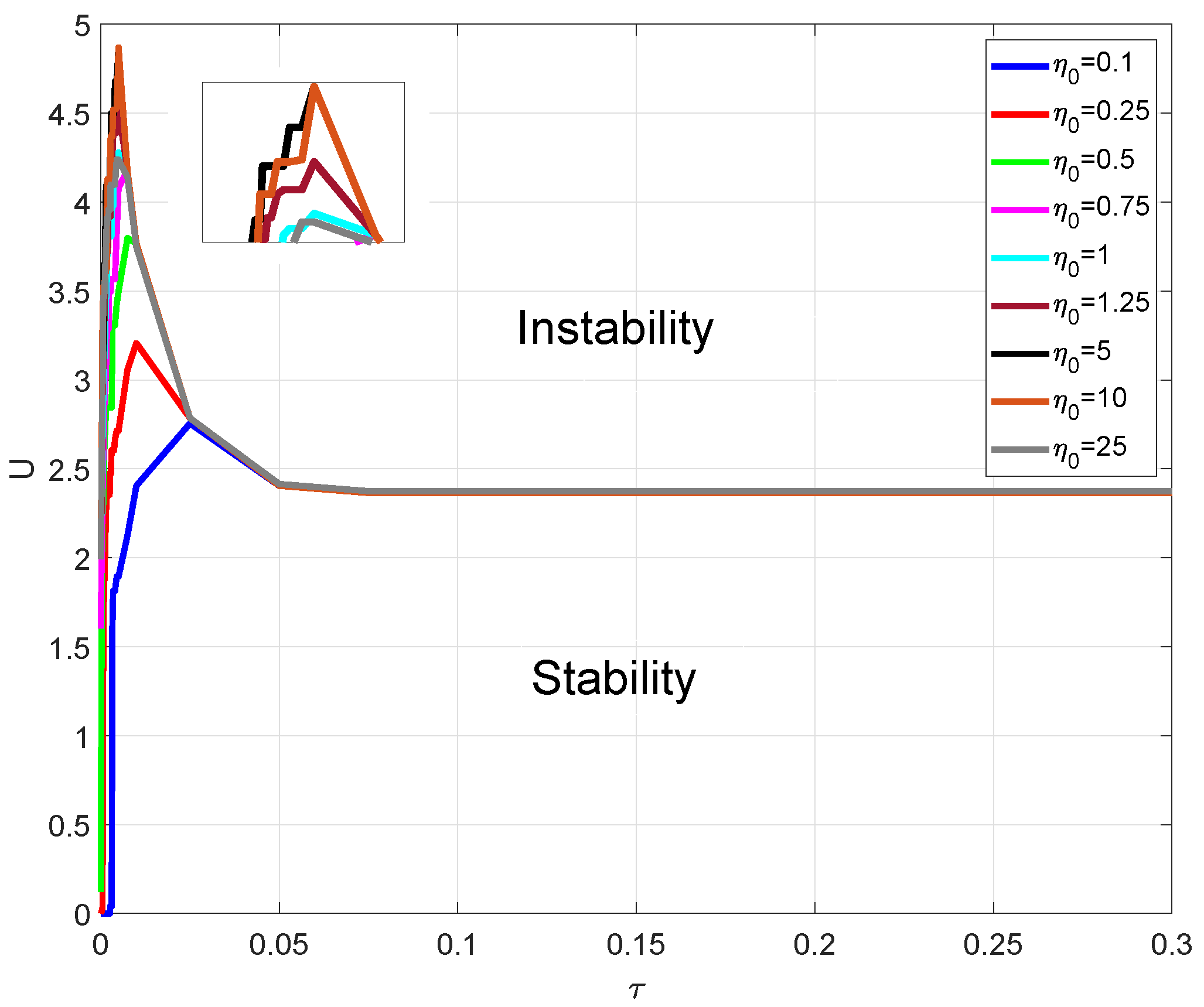
For the DDF models, the role of the external parameter at fixed
is played by the Prandtl number
. For the air, we consider the following values of
: 0.674 (corresponds to 273.15 K), 0.683 (corresponds to 303.15 K), 0.703 (corresponds to 343.15 K) and 0.724 (corresponds to 433.15 K). In
Figure 4, the plots of the boundaries of stability domains are presented. As can be seen, the values of
do not seriously affect the area of the domain. So, the physically correct temperature values do not seriously affect the stability of such DDF models; it depends only on values of
U and relaxation time. It must be noted that the smallest areas occur for the model from [
32], which is based on the D2Q17 lattice. For both DDF models, the areas of domains decrease with the increase of
. As for the multi-speed models, the largest values of
U correspond to the interval
. It must be noted that the constructed models correspond to the case of viscous flows, which is described by the Navier–Stokes system, and in the expression for viscosity obtained by the application of Chapman–Enskog expansions, the dynamic viscosity is directly proportional to the value of relaxation time. So, the case of small values of
corresponds to a small value of viscosity. So, the largest values of
U correspond to the case of inviscid flows. In most of the works, the models are constructed for the simulation of this type of flow in order to simulate many interesting effects, such as shock and rarefication waves, instabilities, etc., and the best stability properties are also observed for the conditions typical for these flows.
4. Numerical Experiments
In the presented section, we try to compare the considered models, applied to the numerical solution of nonlinear 2D problems: the Riemann problems and KHI simulation. All parameter values from the stated conditions are chosen from the literature where these problems are stated.
The computations are performed using the finite-difference off-lattice scheme with the use of the technique based on the splitting of physical processes (e.g., see [
46,
47,
48,
49,
50,
51]). Let us consider a time grid constructed with the step
and nodes
. According to the splitting conception, on one time step
the two processes are considered separately. First, the collision of particles, which is described by the following system:
with the initial condition
. Second, their free streaming after the collision, which is described by the following system of linear advection equations:
which is solved with the initial condition
. By applying this technique, we can use different schemes for the implementation of both stages in order to improve the stability and accuracy of the computational procedure.
Let us consider the spatial grid with nodes
, constructed with step
h on both variables. For the discretization of the linear system (
19) we use the following parametric scheme, constructed as a combination of schemes with second-order central differences and first-order upwind differences:
where
and
and
is the dimensionless parameter. By choosing the proper value of this parameter, we can compensate the effects of numerical dispersion, typical for schemes with central differences, and the effect of numerical dissipation, typical for schemes with upwind differences [
52]. The same approach is used for the equations of the DDF model.
For the implementation of (
18) the explicit Euler method is used:
The computations are performed in the case of small value of CFL number () in order to exclude any numerical instabilities.
As an example of the multi-speed model, we consider the model from [
19], and as a DDF model, the model from [
24] is used. The model from [
13] is not considered due to the large number of equations; the model from [
32] is not considered due to the small areas of the stability domain (see
Figure 4).
The parameter values are selected in such a way that the solutions of kinetic equations will be stable (the parameter values correspond to the internal points of the stability domains). For considered problems, the following parameter values are used: For the model from [
19],
,
,
and
. For the model from [
24],
,
l and
are the same. For all problems,
is used as the value of relaxation time in order to reproduce the inviscid flow because, as is mentioned above, the dynamic viscosity for this model is proportional to
[
19]. For the DDF model from [
24], we set
and
,
is computed as
. For all problems, the value
is used.
The initial-boundary-value problems considered in this section are stated in the unbounded spatial domain (2D for the KHI problem and 1D for Riemann problems). In order to solve such problems numerically, the computational domain is defined as a rectangle. The effects of infinite boundaries are simulated by periodic or extrapolated boundary conditions.
4.1. Riemann Problems
Let us consider three problems, stated in the infinite interval with the following initial conditions for macrovariables:
(a) Problem with discontinuous velocity:
(b) Problem with discontinuous density:
where temperature
T is related with the internal energy according to the used equation-of-state:
.
(c) Sod’s problem, which is widely used as a test for solvers in gas dynamics [
53,
54]:
This initial condition leads to the solution with a right-propagating shock, a right-propagating contact wave and a left-propagating rarefication wave.
Stated problems can be solved exactly [
55], so they can be considered as powerful tools for testing numerical schemes and their implementations.
For numerical realization, we consider the finite interval on variable x: , where the grid with step h and N nodes is constructed. We perform computations in the rectangular domain, where the interval on y is defined as . On the upper and lower boundaries, the periodic boundary conditions are stated. At left and right boundaries, the extrapolated conditions are stated: , , and the same conditions are stated for . The initial values of and are computed from the values of equilibrium distributions computed from the initial conditions stated for macrovariables.
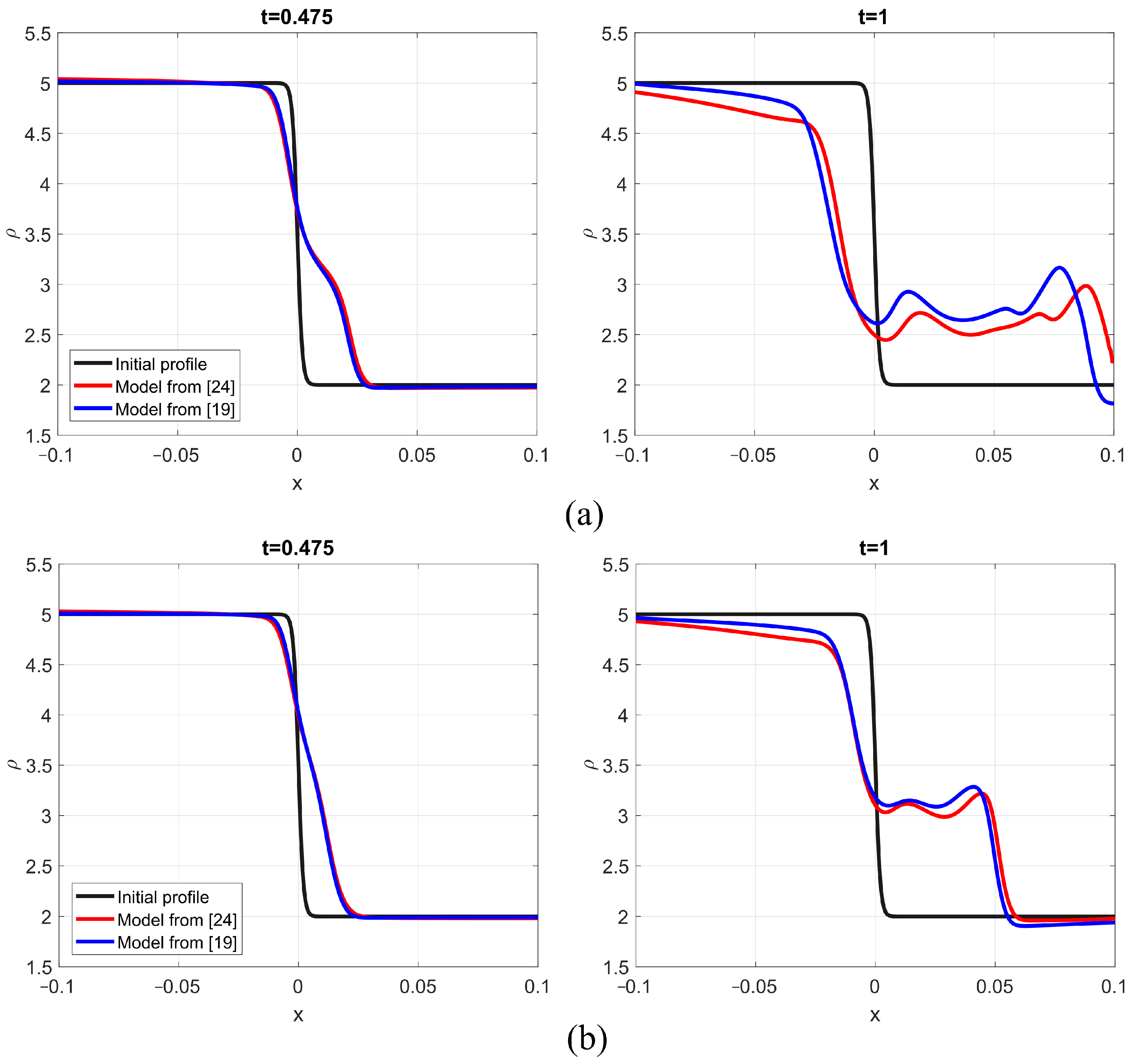
The results demonstrated in
Figure 5,
Figure 6 and
Figure 7 are obtained in the case of
for the spatial grid with
at the endpoints of time intervals. For problem 1, the time interval
is considered, and for problems 2 and 3, the intervals
and
are used. Some minor numerical artifacts, associated with small-amplitude osclillations near the contact line, are observed according to the presence of the term with a second-order central difference in the finite-difference scheme (
20). As can be seen, both models lead to very close results.
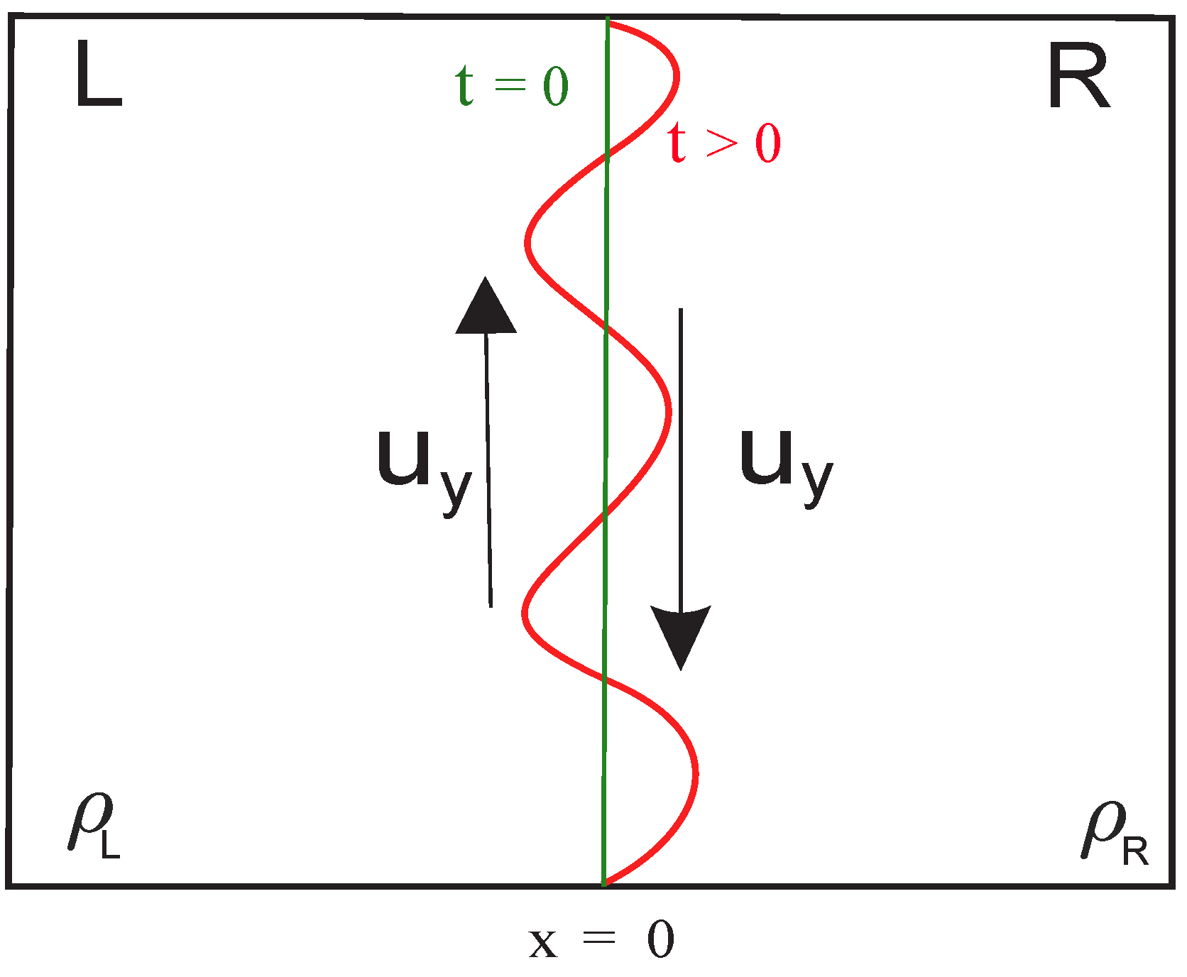
4.2. Kelvin–Helmholtz Instability
The KHI occurs in a system when two immiscible fluids flow at different tangential velocities (e.g., in opposite directions) and there are exist small perturbations near the interface (
Figure 8). Such perturbations between two fluids grow in time and may evolve into turbulent mixing through nonlinear interaction. The KHI is observed in nature and industry and plays an important role in such processes as supernova dynamics, interaction of the solar wind with the Earth’s magnetosphere, cloud dynamics, etc. [
56,
57,
58]. Furthermore, this type of instability is a typical example of non-equilibrium flow, and its non-equilibrium effect is significant near the interface, where the instabilities grow, which is why the kinetic equations are intensively used in the analysis of its evolution [
59].
For the numerical simulation, the system, formed by two immiscible fluids with different initial densities and tangential velocities, is considered (see
Figure 8 for schematic representation). The interface in the initial time moment is represented by the straight line, which corresponds to
.
The considered models are not adopted for multiphase simulations or simulations with interfaces between flows with different physical characteristics. So, the effect of the interface is simulated by the initial condition with the steep profile [
60]. The solution corresponding to this condition evolves as a model that reproduces the dynamics of a system with immiscible fluids. So, LBM in this situation is considered as shock-capturing method.
The following initial conditions are stated [
59,
60]:
where
,
are constants corresponding to densities of fluids,
and
are corresponding tangential velocities,
and
are positive constants, which characterize the width of density and velocity transitional layers,
is the frequency of the perturbations of the interface,
characterizes its amplitude and
is the initial pressure.
For the computations, we consider the rectangular domain , in the case of . The following parameter values are used: , , , , and . On all boundaries, the zeroth-order extrapolation conditions, as for the Riemann problems, are stated. The distribution functions in the initial time moment are computed as the equilibrium distributions, computed on the initial conditions, stated for macrovariables. The computations are performed for the time interval . A spatial grid consists of nodes.
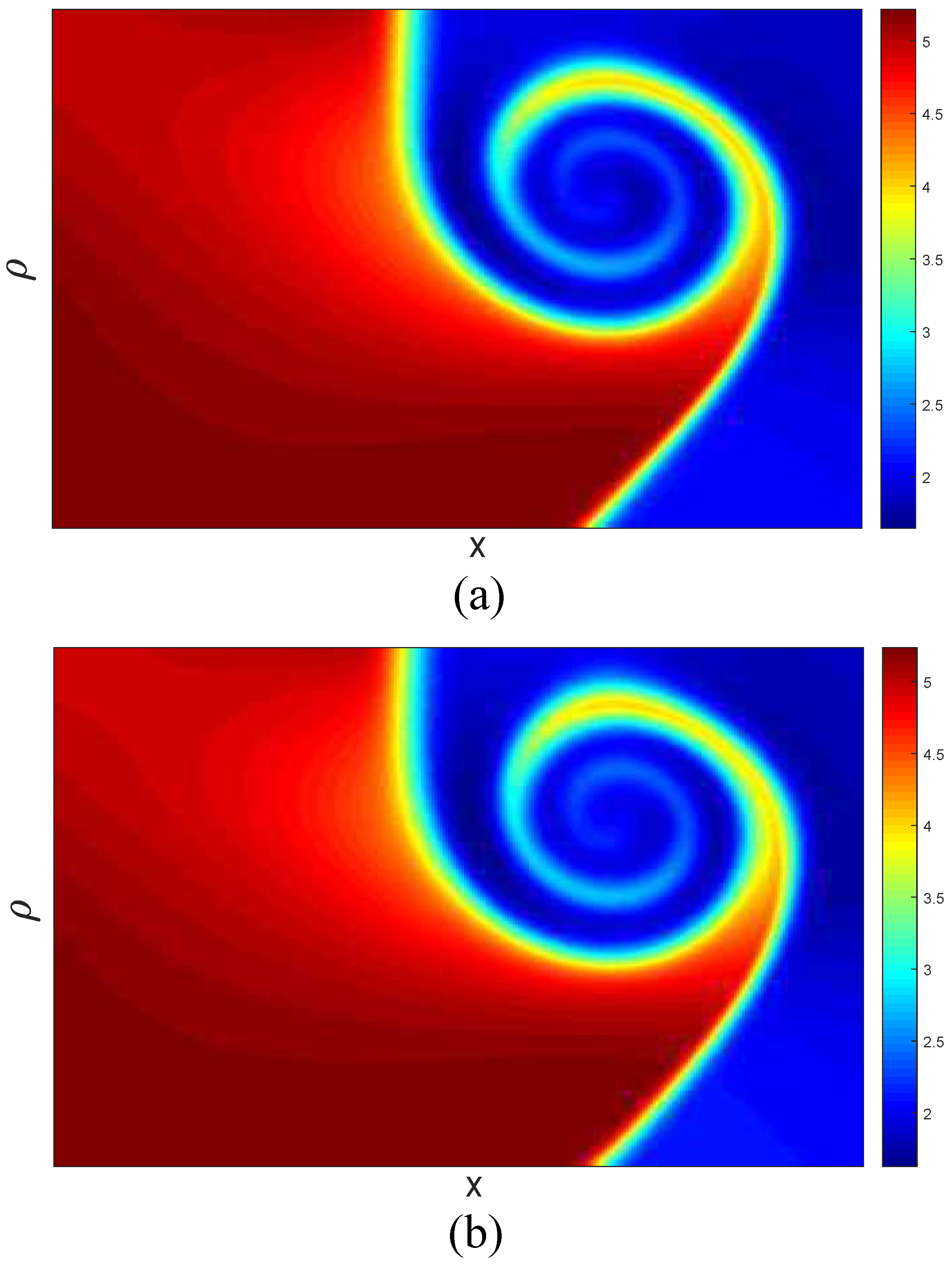
In
Figure 9, the contour plots of
in moment
for values
,
and
are presented. As can be seen, the results obtained by both models are close to each other, and the coordinates of the vortex center are similarly predicted by both models.
In
Figure 10, the plots of density profiles corresponding to the fixed value
are presented for the values
and
in the cases of various values of
k, which characterize the frequency of interface perturbation. As it can be seen, the solutions obtained by both models lead to similar profiles with weak discrepancies in values of
(not larger than 0.2). The profiles, obtained for various values of
, are presented in
Figure 11 for the case of
,
. As can be seen, both models lead to similar profiles (discrepancies on values of
are not larger than 0.25 (
%)). It should be noted that the complete investigation of parameters influence on the solution of this problem is performed and discussed in detail in [
60]. In the presented paper, we focus attention only on the comparison of numerical solutions obtained by different models based on kinetic equations.
For the estimation of
, obtained by kinetic models in a whole spatial domain, the averaged value can be used:
The computation of this characteristic is performed by the following quadrature formula:
where
are computed from the values of distribution functions. In
Figure 12, the plots of
, obtained for
and
for different values of
k, are presented. In
Figure 13, the plots for the case of
,
and different values of
are presented. As can be seen, the values of the averaged density obtained by both models are close to each other. The highest deviations of values of
are not larger than 0.25.
5. Conclusions
In the presented paper, the analysis of discrete velocity kinetic models used in the LBM simulation of compressible flows in the LBM for cases of varied specific heat ratios in the equation-of-state is performed. The popular multi-speed and DDF models, presented in the literature, are compared. In the theoretical part, the stability analysis of steady-state solutions associated with steady flow regimes is performed. The stability analysis problem is reduced to the analysis of zero solutions of linear systems of ordinary differential equations. These systems are obtained after the linearization of kinetic equations near the steady-state solution. The analysis is based on the construction of stability domains in parametric space. The results obtained for different models are compared. In the practical part, the selected models are applied to the simulation of compressible flows. The Riemann problems and the simulation of KHI are considered. For the numerical simulations, the parametric finite-difference scheme is used. As is demonstrated, different kinetic models lead to close numerical solutions for both types of problems.
As the main results, the following conclusions can be formulated:
1. The procedure for the linear stability analysis of compressible discrete kinetic models is proposed, and stability domains are constructed. The approach is based on the considering of steady-state solutions associated with steady flow regimes. According to the proposed procedure, we reduce the analysis of steady-state solutions of nonlinear kinetic equations to the analysis of zero solutions of linear systems of ordinary differential equations. According to the stability criterion, these solutions are asymptotically stable if and only if the real parts of the eigenvalues of the matrices of the corresponding systems have negative real parts. With the use of this criterion, we can construct the stability domains in the parametric space. Only the stability of solutions of kinetic equations, which formed the model, is analyzed. In practice, the numerical instabilities associated with the used computational schemes also take place.
The proposed approach to analysis can be used as an effective tool for the theoretical comparison of different kinetic models used in the LBM in other fields, for example, for multiphase and magnetohydrodynamic simulations. It allows for the possibility to define the range of free parameters presented in the models.
2. The effects of the input parameters on the boundaries of the stability domains are analyzed. For the models from [
13,
19], the areas of the domains can be enlarged by the increase of
(see
Figure 2,
Figure 3 and
Figure 4). For the model from [
19], the upper values of
U, which provide stability, decrease with the increase of
(
Figure 2). However, for the model from [
13], this value for
can be approximated by the constant 2.4 (see
Figure 3). For the DDF models, the value of
very slightly affects the boundaries of the stability domains (see
Figure 4).
For both types of models, the largest value of
U occurs for the small values of
(
). This means that the models provide the most stable results if the semi-inviscid flows are simulated. Despite the fact that the considered models are developed in order to mathematically reproduce Navier–Stokes equations, which describe viscous flows, in most works they are used for the simulation of inviscid flows, which are described by the Euler equations. The expression for viscosity is obtained by applying the Chapman–Enskog asymptotic expansion method. As it is demonstrated, the dynamic viscosity
is proportional to
(that is why the inviscid flows are simulated by the use of a small relaxation time). For example, for the model from [
13] the following expression takes place:
The case of the small value of corresponds to the small value of . So, in the presented work, it is demonstrated that these models are better suited to be used in practice for the simulation of inviscid flows because, in this case, they lead to larger stability intervals on values of U.
3. As it is obtained after numerical experiments for the case of the air flow, the smallest areas of the domains are observed for the model from [
32] and for the model from [
19] at small values of
. The best stability properties (largest areas) occur for the model from [
13]. However, this model consists of 65 equations, so it is not optimal for practical computations.
4. As is demonstrated in the numerical experiments on the simulation of compressible flows, both types of models (multi-speed and DDF) provide close values for macrovariables. So, in practice, any of the constructed models can be used. However, their parameters should be defined based on the stability conditions obtained after the analysis of stability domains.
5. The presented study can be considered as the first stage of the analysis of models used in the LBM for compressible flow simulations. The presented approach to linear stability analysis can be used for different models of different physical phenomena. In the LBM over the last decades, multiparametric methods, which improve stability, have been proposed; for example, MRT methods [
38,
61,
62] and cascaded models [
63,
64,
65]. The stability of such schemes and their variations will be analyzed in future studies.


