Article

Anomalous Solute Transport Using Adsorption Effects and the Degradation of Solute

Department of Mathematical Modeling, Faculty of Mathematics, Samarkand State University, 15, University Blvd., Samarkand 140104, Uzbekistan
*
Author to whom correspondence should be addressed.
Computation 2023, 11(11), 229; https://doi.org/10.3390/computation11110229
Submission received: 2 July 2023 / Revised: 13 October 2023 / Accepted: 15 October 2023 / Published: 16 November 2023
(This article belongs to the Special Issue Computational Techniques for Fluid Dynamics Problems)

Abstract

:
In this work, anomalous solute transport using adsorption effects and the decomposition of solute was studied. During the filtration of inhomogeneous liquids, a number of new phenomena arise, and this is very important for understanding the mechanisms of the filtration process. Recently, issues of mathematical modeling of substance transfer processes have been intensively discussed. Modeling approaches are based on the law of matter balance in a certain control volume using additional phenomenological relationships. The process of anomalous solute transport in a porous medium was modeled by differential equations with a fractional derivative. A new mobile—immobile model is proposed to describe anomalous solute transport with a scale-dependent dispersion in inhomogeneous porous media. The profiles of changes in the concentrations of suspended particles in the macropore and micropore were determined. The influence of the order of the derivative with respect to the coordinate and time, i.e., the fractal dimension of the medium, was estimated based on the characteristics of the solute transport in both zones. The hydrodynamic dispersion was set through various relations: constant, linear, and exponential. Based on the numerical results, the concentration fields were determined for different values of the initial data and different relations of hydrodynamic dispersion.

1. Introduction

An important and complex issue in the study of anomalous solute transport is scale-dependent dispersion [1,2,3,4]. The essence of scale-dependent dispersion is that the dispersion power or dispersion coefficient changes with distance or time when using the convection—dispersion equation to describe the process of anomalous solute transport in porous media [3,5,6,7,8,9,10,11].
Most analytical studies related to scale-dependent dispersion are based on the convection—dispersion equation. However, in recent years many researchers have often questioned the use of the convection—dispersion equation, since it cannot adequately explain anomalous transport in inhomogeneous porous media, and alternative models have been proposed. The mobile—immobile model differs from the convection—dispersion model in that it consists of the presence of a stagnant region in a porous medium and the exchange of dissolved substances between mobile and stagnant regions, which explains the early entry and long transport time of solutes. The solute flux in the mobile—immobile model is proportional to the concentration and the difference between these two areas. More detailed information related to the analysis of the mobile—immobile model can be found in [12]. It was shown that the mobile–immobile model can better describe the transport of dissolved substances in both homogeneous and inhomogeneous porous media than the convection—dispersion equation [13,14,15,16,17,18,19].
The first-order mass transfer in the mobile—immobile model is considered to be rate-limited when the exchange time scale is equal to or exceeds the characteristic advection time scale through the medium [20,21]. Some studies describe how rate-limited transport processes may be better suited to describing solute transport in a macro dispersion experiment than a macro dispersion model [20,22]. Another widely used velocity-limited mass transfer model is the physical diffusion model, in which the diffusion into and out of a fixed zone is described by Fick’s law [23,24]. However, the diffusion model is limited to structured soils with geometrically well-defined aggregates [12]. In addition, different expressions for the first order mass transfer rate can be obtained for a diffusion model with some idealized aggregate shapes [23].
It should be noted that the mobile—immobile model considered above uses a lumped unified velocity to describe a complex mass transfer process. However, for natural soils or complex and heterogeneous aquifers characterized by microscale variations in the properties of the porous media, the rates and types of mass transfer differ greatly [21,24]. The single-speed mobile—immobile model cannot accurately describe the nature of long-term transport caused by multiple and simultaneous mass transfer processes [19,25]. A multi-velocity mobile—immobile model was developed using a distribution of mass transfer coefficients in combination with the convection—dispersive model of solute transport [24]. The continuum of velocities in a memory function and the resulting equations of the mobile—immobile model with several velocities were defined as a pair of coupled deterministic partial differential equations in continuous time and space with one derivative with respect to time [21]. The single-velocity mobile—immobile model and diffusion models for various geometries, as special cases of the multi-velocity mobile—immobile model, were studied [24,25,26,27].
The mobile and immobile model separates the liquid phase of a porous medium into a mobile and a stationary region. It is assumed that the convective—dispersive transport is limited to the region of the mobile fluid and that the exchange of the solutes between these two regions of the fluid can be described as a first order process. The solid phase of the porous medium is also divided into two adsorption centers that are instantly balanced with the mobile and immobile liquid regions, respectively. The adsorption of a solute by a solid phase is described by a linear isotherm and the degradation of a solute in both liquid and solid phases is considered a first order process. To maintain the generality of the model, different degradation coefficients were taken into account in the mobile and stationary liquid regions as well as in the mobile and stationary adsorbed phases [28]. The mobile—immobile (M&IM) model was developed on the basis of the two-region or two-site model, which divides heterogeneous porous media into mobile and immobile regions [13,29]. The solute transport and kinetic equations were considered to analyze reactive solute transport and the analytical method was used to describe the results [30].
In this study, the process of anomalous solute transport in a porous medium is modeled by differential equations with fractional derivatives. A new “mobile—immobile” model is proposed to describe the anomalous solute transport with a scale-dependent dispersion in inhomogeneous porous media.
The mobile region is the zone with the moving fluid and the immobile region is the zone with the stationary fluid. The mobile region governs flow transport processes, i.e., advection and the dispersion process, and the stagnant or immobile region accounts for the first-order lumped mass transfer between mobile and immobile regions. The profiles included in the concentrations of suspended particles in the macropore and micropore were determined. The influence of the order of the derivatives with respect to the coordinate and time on the characteristics of the solute transport in both zones was estimated. In the zone with the immobile liquid, the transfer process is described by a kinetic equation accounting for adsorption, where, unlike in other well-known works, the anomalous process is also taken into account. In the zone with the mobile liquid, a convective—diffusion equation is used, taking into account the anomalous diffusion process. Further, we use the “mobile” and “immobile” zones, which means the zones with mobile and immobile fluid are studied and presented in the results as graphs.

2. Materials and Methods

2.1. Formulation of the Problem

The environment consists of two zones, one is mobile, i.e., porous medium, where the liquid is mobile, and the other is immobile, where the liquid is immobile. Diffusion solute transport occurs in both zones (See Figure 1).
The model of anomalous solute transport is written as [29,30,31]:
θ m + f ρ b k d c m t = θ m x D m ( x ) β c m x β v m θ m c m x ω c m c i m θ m μ l m + f ρ b k d μ s m c m ,
θ i m + ( 1 f ) ρ b k d α c i m t α = ω ( c m c i m ) θ i m μ l i m + ( l f ) ρ b k d μ s i m c i m
where θ m ,   θ i m are porosity coefficients, c m and c i m are the concentrations of dissolved substances in the mobile and immobile zones, respectively, v m is the fluid velocity, ω is the first-order mass transfer coefficient, f and l f represent the proportions of adsorption centers that are instantly balanced with the areas of mobile and immobile liquid, respectively, ρ b is the density of the porous medium, k d is the distribution coefficient of the linear adsorption process, μ l m and μ l i m are the degradation coefficients of the dissolved substance in the mobile and immobile zones, respectively, μ s m and μ s i m are the degradation coefficients of the adsorbed substance in the mobile and immobile zones, respectively, x is the spatial coordinate, t is the time, and D m ( x ) is the coefficient of hydrodynamic dispersion in the moving zone expressed as [32]:
D m ( x ) = ϕ ( x ) v m + D 0
ϕ ( x ) is the dispersion and D 0 is the diffusion coefficient.
The parameter values are taken as [30] and the orders of the derivatives are considered as: 0 < α 1 , 0 < β 1 . In contrast to [30], here we take other dimensions as D m ( x ) = m β + 1 / s . θ i m + 1 f ρ b k d = s α 1 represents fractal dimensions of the parameters.
Using R m = θ m + f ρ b k d , R i m = θ i m + ( 1 f ) ρ b k d , A 1 = θ m μ l m + f ρ b k d μ s m , and A 2 = θ i m μ l i m + ( 1 f ) ρ b k d μ s i m , Equations (1) and (2) can be transformed into a simpler form as follows:
R m c m t = θ m x D m ( x ) β c m x β v m θ m c m x ω c m c i m A 1 c m ,
R i m α c i m t α = ω ( c m c i m ) A 2 c i m ,
where R m , R i m are the retardation factors in the moving and stationary zones, respectively.
For mobile and immobile models with scale-dependent dispersion, the dispersion is not a constant, but a function of distance. Here, as in previous experimental and theoretical studies [33], we use linear and exponential dispersion functions. Distance-dependent linear variance increases without limit with distance, while distance-dependent exponential variance initially increases with distance and eventually approaches an asymptotic value. The formula for linear distance-dependent dispersion is:
ϕ ( x ) = k x ,
where k is the slope of the ratio of dispersion to distance (dimensionless). The exponential dependence of dispersion on distance is expressed as:
ϕ ( x ) = a 1 e b x ,
where a is the asymptotic value at infinity and a , b are positive constants.
Consider the problem of a fluid with a substance concentration, c 0 , movable zone from x = 0 . Initially, both the zones are filled with pure (without substance) liquid.
The initial and boundary conditions for this setting are:
c m ( 0 ,   x ) = 0 ,   c i m ( 0 ,   x ) = 0 ,
c m ( t ,   0 ) = c 0 ,   c m ( t ,   ) = 0 .

2.2. Solution Procedure

For the numerical solution of Equations (3)–(9), we use the finite difference method [34]. In the domain, Ω = 0 x , 0 t T introduces a uniform grid method, ω h τ = ( x i , t j ) ,       x i = i h ,       i = 0 , N ¯ ,     h = L / N ,     t j = j τ ,     j = 0 , M ¯ ,   τ = T / M , where h is the grid step size at coordinate x , τ is the grid step at time t , and L is the characteristic length of the porous medium, chosen so that the concentration field does not reach x = L within the considered time range.
To approximate the fractional time derivatives, we use the schemes given in [35,36,37]. The difference approximation of the kinetic equation (Equation (5)) is written as:
R i m Γ ( 2 α ) τ α l = 0 j 1 ( c i m ) i l + 1 ( c i m ) i l j l + 1 1 α j l 1 α + ( c i m ) i j + 1 ( c i m ) i j = = ω ( ( c m ) i j ( c i m ) i j ) A 2 ( c i m ) i j .
For the three cases of dispersion coefficients (constant, linear, asymptotic exponential), Equation (4) is approximated in the following forms.
  • Constant case
D m ( x ) = ϕ ( x ) v m + D 0 ,   ϕ ( x ) = 0 ,   D m ( x ) = D 0
R m c m t = θ m D 0 β + 1 c m x β + 1 v m θ m c m x ω c m c i m A 1 c m ,
R m ( c m ) i j + 1 ( c m ) i j τ = θ m D 0 Γ ( 3 ( β + 1 ) ) h β + 1 l = 0 i 1 ( c m ) i ( l + 1 ) j 2 ( c m ) i l j + ( c m ) i ( l 1 ) j × l + 1 2 ( β + 1 ) l 2 ( β + 1 ) v m θ m ( c m ) i + 1 j ( c m ) i 1 j 2 h ω ( ( c m ) i j ( c i m ) i j ) A 1 ( c m ) i j ,
2.
Linear case
D m ( x ) = ϕ ( x ) v m + D 0 ,   ϕ ( x ) = k x ,   L 1 = k v m ,   D m ( x ) = k x v m + D 0 .
R m c m t = θ m x k x v m + D 0 β c m x β v m θ m c m x ω c m c i m A 1 c m ,
R m c m t = θ m k v m β c m x β + k x v m + D 0 β + 1 c m x β + 1 ( v m θ m ) c m x ω c m c i m A 1 c m ,
R m ( c m ) i j + 1 ( c m ) i j τ = θ m k v m ( c m ) i + 1 j β · ( c m ) i j Γ ( 2 β ) h β + θ m k i h v m + D 0 × l = 0 i 1 ( c m ) i ( l + 1 ) j 2 ( c m ) i l j + ( c m ) i ( l 1 ) j l + 1 2 ( β + 1 ) l 2 ( β + 1 ) Γ ( 3 ( β + 1 ) ) h β + 1 v m θ m ( c m ) i + 1 j ( c m ) i 1 j 2 h ω ( ( c m ) i j ( c i m ) i j ) A 1 ( c m ) i j .
3.
Exponential case
D m ( x ) = ϕ ( x ) v m + D 0 ,   ϕ ( x ) = a ( 1 e b x ) ,   D m ( x ) = a ( 1 e b x ) v m + D 0 .
R i m c m t = θ m x ( a v m ( 1 e b x ) + D 0 ) β c m x β v m θ m c m x ω c m c i m A 1 c ,
R i m c m t = θ m ( a v m a v m e b x + D 0 ) β + 1 c m x β + 1 + ( a b v m e b x ) β c m x β v m θ m c m x ω c m c i m A 1 c ,
R m ( c m ) i j + 1 ( c m ) i j τ = θ m ( a υ m + a υ m e i h + D 0 ) Γ ( 3 ( β + 1 ) ) h β + 1 l = 0 i 1 ( c m ) i ( l + 1 ) j 2 ( c m ) i l j + ( c m ) i ( l 1 ) j × l + 1 2 ( β + 1 ) l 2 ( β + 1 ) + θ m ( a b υ m e b i h ) ( c m ) i + 1 j β ( c m ) i j Γ ( 2 β ) h β v m θ m ( c m ) i + 1 j ( c m ) i 1 j 2 h ω ( ( c m ) i j ( c i m ) i j ) A 1 ( c m ) i j .
The initial and boundary conditions are approximated as follows:
( c m ) i 0 = 0 ( c i m ) i 0 = 0 ,
( c m ) 0 j = c 0 ,     ( c m ) N j = 0 .
where N is a sufficiently large number for which the equation c N j = 0 is approximately satisfied.

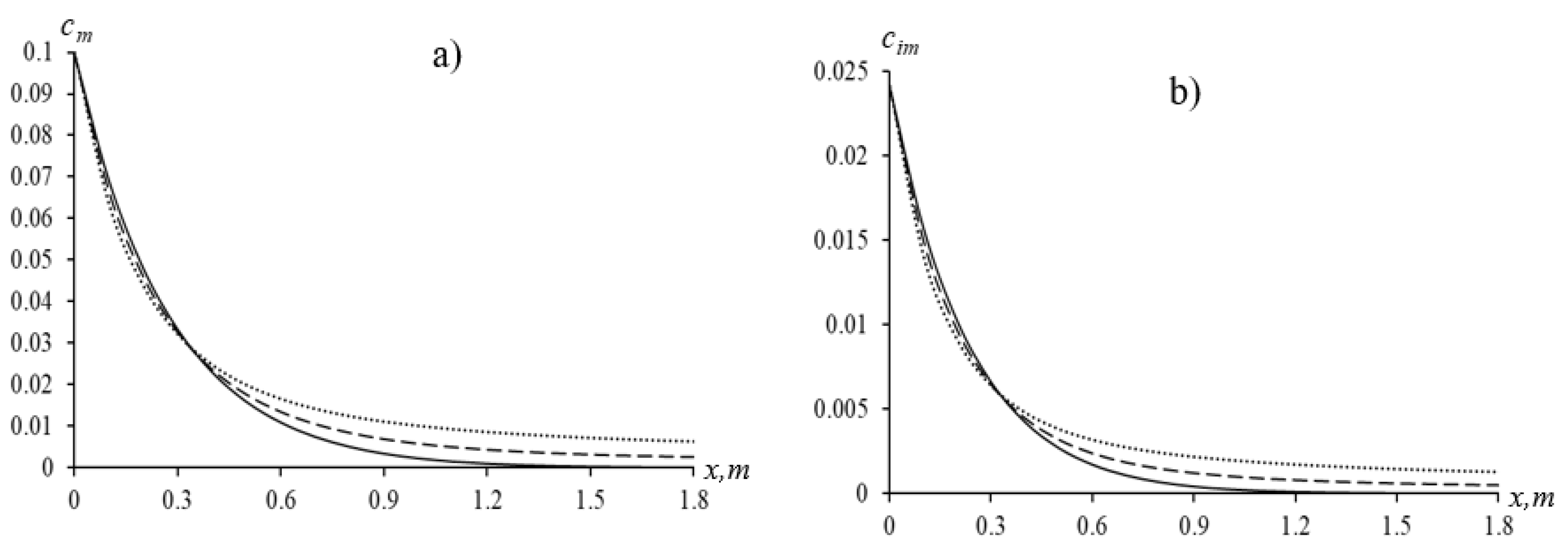
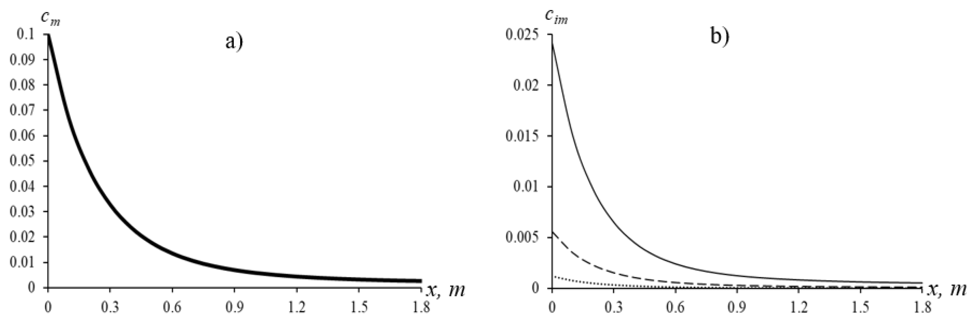
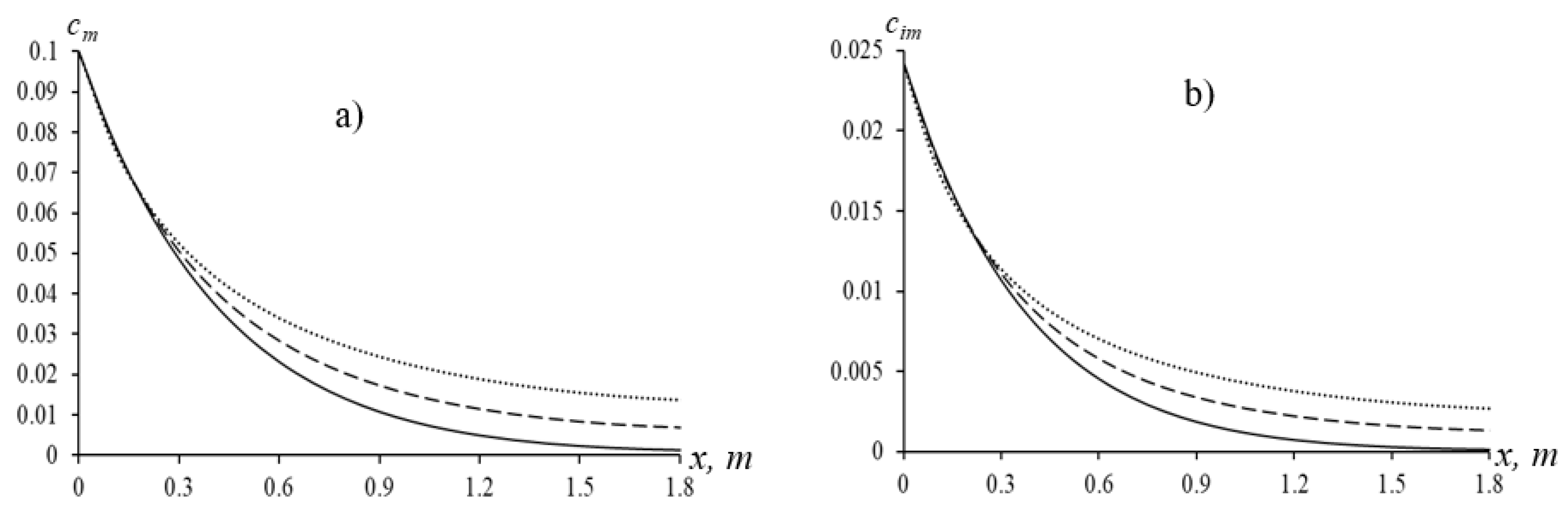
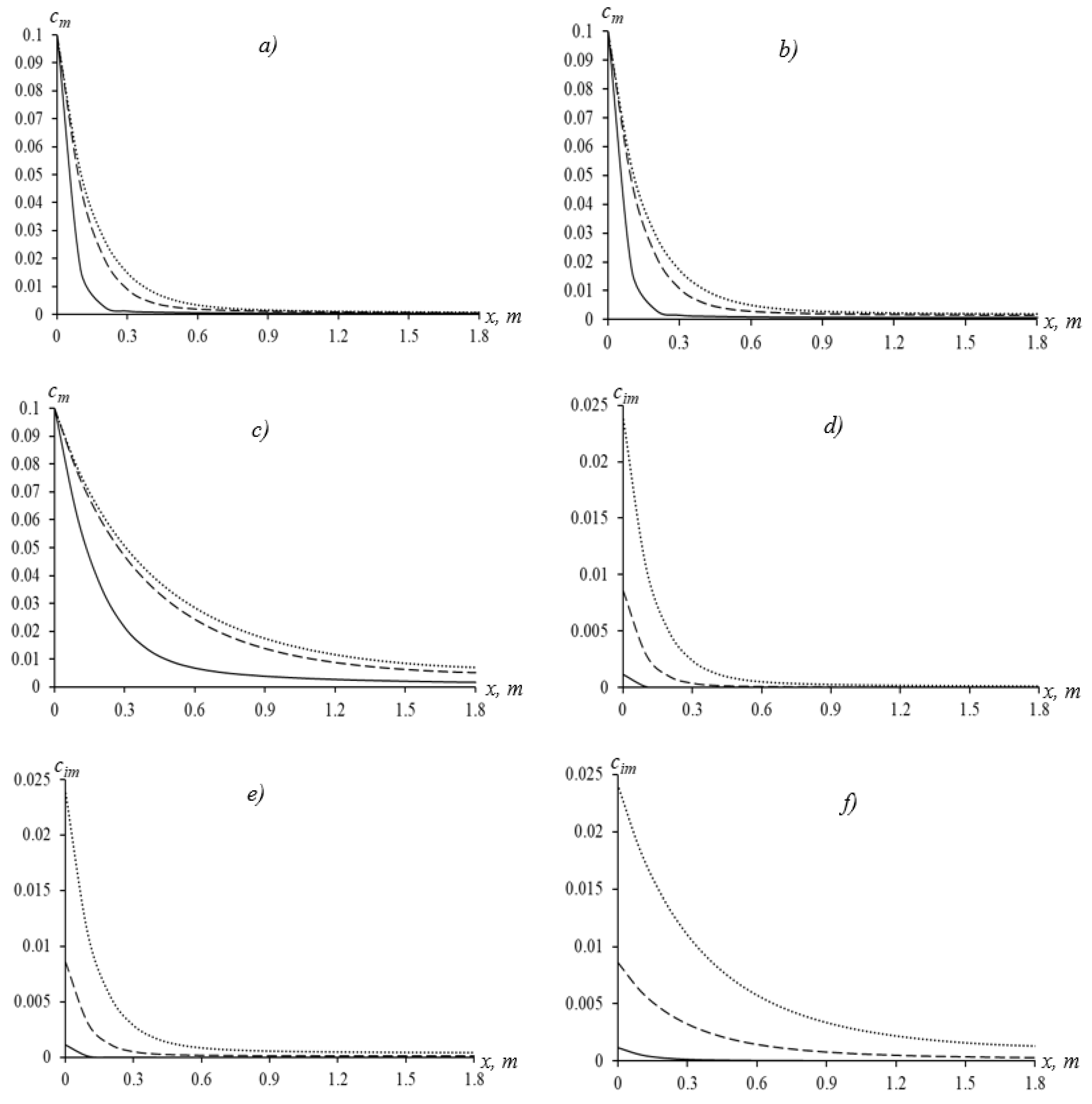
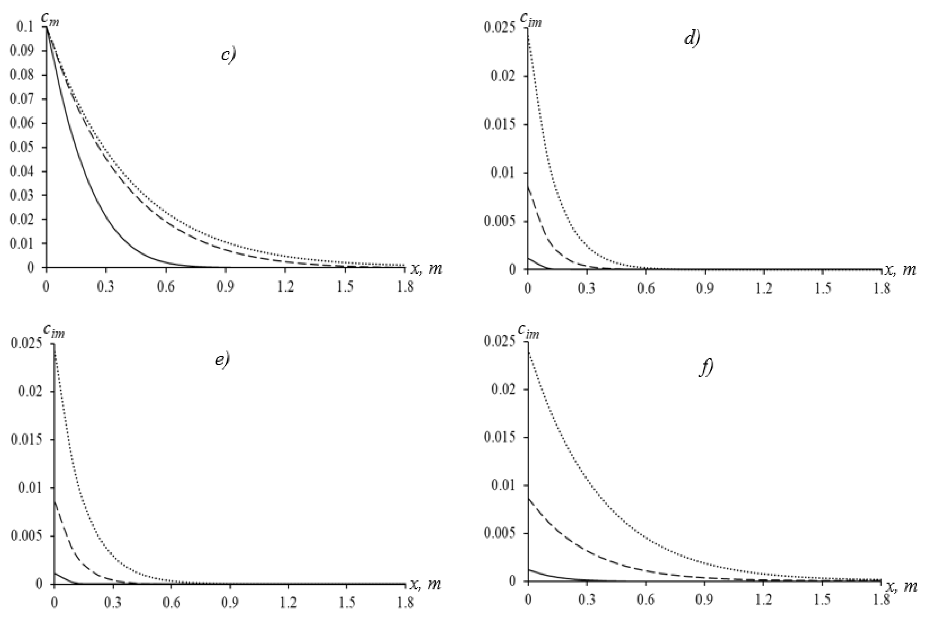
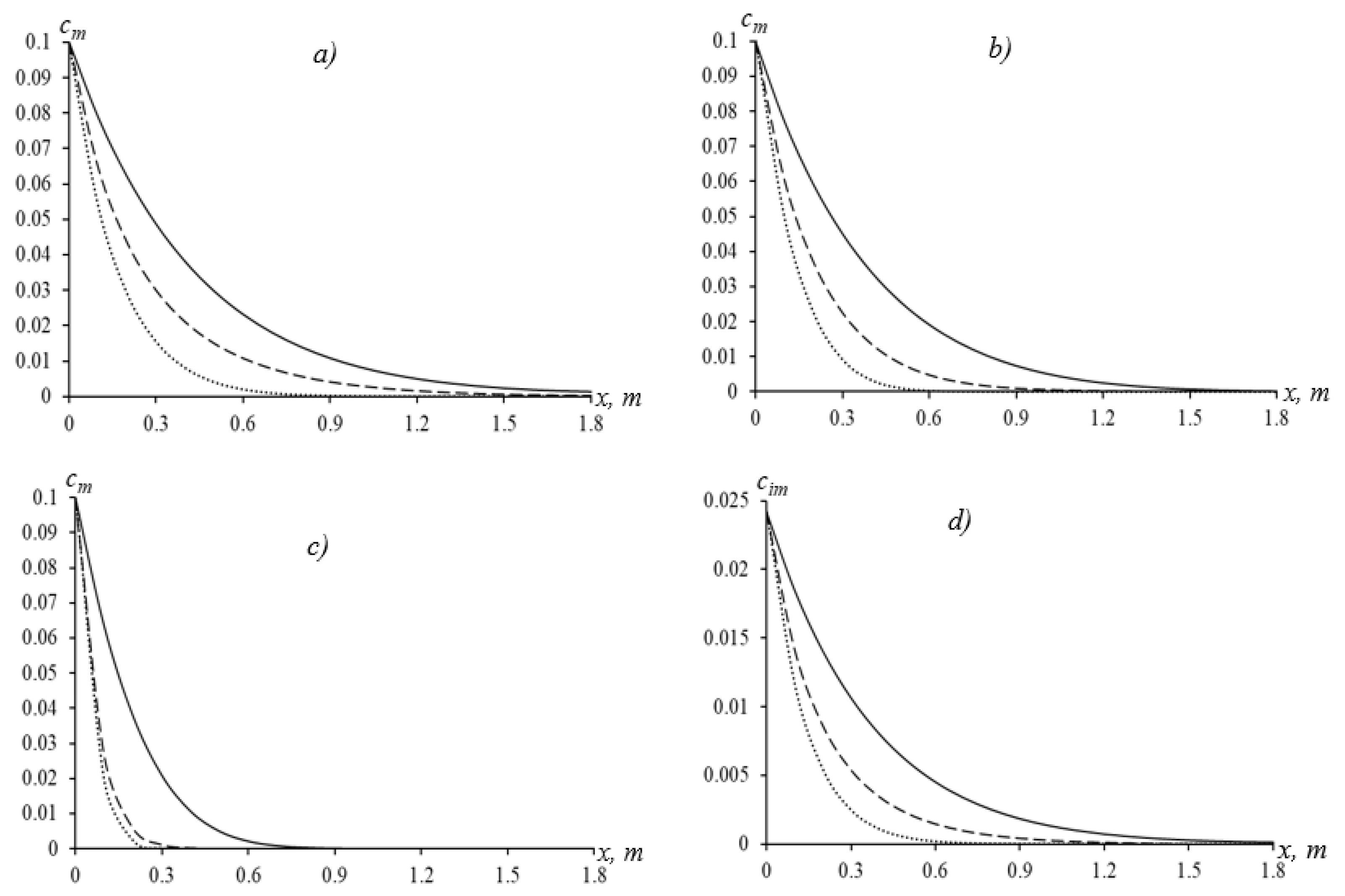
3. Results and Discussion

The classical case of the newly proposed model was compared with the results obtained from previous work [29] for the constant case and is shown in Figure 2. Here, α = 1 and β = 1 are fixed in the fractional derivative. It can be seen from the figure that the new model in reduced cases coincides exactly with the solution of the problem in the classical case.
The following values of the initial parameters were used to analyze the new results [29,30]: θ m = 0.4     , θ i m = 0.1 , ρ b = 1000 , k d = 10 6 , μ l m = 10 3 , μ s m = 10 4 , μ l i m = 10 6 , μ s i m = 10 8 , v m = 10 4 , ω = 10 5 , D 0 = 10 5 , T = 3600 , f = 0.7 , k = 0.5 , a = 1 , b = 0.5 . These values were used to solve Equations (10)–(13). Three different hydrodynamic dispersion coefficients, namely, constant, linear, and exponential coefficients, are discussed for the concentration profiles of mobile and immobile zones, and the results are presented in the figures.
Figure 3a–d shows the changes in substance concentrations for various hydrodynamic dispersion coefficients (constant, linear, and asymptotic) and various α and β values. With a decrease in the order of the derivative for β 1 in the diffusion term of the mass transfer equation, a wider distribution of the concentration profile in the mobile and immobile zones is observed.
  • Constant case
Figure 4, Figure 5, Figure 6 and Figure 7 depict a case in which the hydrodynamic dispersion coefficient is constant. Figure 4 shows the variation in concentration values in the mobile and immobile zones for different values of β , in which of α = 1 and t = 3600 are fixed values. In this case, the distribution of concentration profiles in both zones becomes wider. Similarly, Figure 5 shows the variation in the concentration value in the mobile and immobile zones for different values of β , in which α = 0.8 and t = 3600 are fixed values. The pattern of the variation is the same as shown in Figure 4.
Figure 6 and Figure 7 show the values of the mobile and immobile zones for β = 1 and β = 0.8 , respectively, with different values of α ( α = 0.8 ,       0.9 , and 1.0 ). In Figure 6a and Figure 7a, the differences in the values of the distribution of concentration profiles are very small (maximum difference is 6.80973 × 10⁻⁵). It can be seen from the figures that the concentration profiles are more widely distributed in the mobile zone, but less widely distributed in the immobile zone.
2.
Linear case
Figure 8, Figure 9, Figure 10 and Figure 11 show the results for a linearly varying hydrodynamic dispersion coefficient.
Figure 8 and Figure 9 depict the change in concentration profiles for different values of β , in which α = 1 and α = 0.8 , respectively. The concentration profiles decrease with respect to the length parameter, which is higher for higher values of β .
Figure 10 and Figure 11 show the concentration profile for the time derivatives α = 0.8 ,       0.9 and 1.0 , fixing β = 1 and β = 0.8 , respectively. These figures show that the concentration profiles are more widely distributed in the mobile zone, while in the stationary zone, on the contrary, they decrease.
3.
Exponential case
The results for the exponential hydrodynamic dispersion coefficient are shown in Figure 12, Figure 13, Figure 14 and Figure 15. With a decrease in the value of β , a wider distribution of concentration profiles in both zones is observed (Figure 12 and Figure 13) for β = 1 and β = 0.8 . Decreasing the order of the time derivative, α , less than 1 in the mass transfer equation, the concentration profiles spread more widely in the mobile zone, but spread less in the stationary zone (Figure 14 and Figure 15).
The results of calculations related to the change in the adsorption values are shown in Figure 16, Figure 17 and Figure 18. As can be seen from Figure 16, a decrease in β from 1 , as in the previous cases, leads to an increase in diffusion effects in both zones. Comparison of these results with the corresponding ones for k d = 10 4 , k d = 10 3 , and k d = 10 2 shows that adsorption leads to a general slowdown in the process of distribution of the substance. The change in the concentration profiles at different adsorption values is shown in Figure 17 and Figure 18. With an increase in the adsorption coefficient, a lagging distribution of concentration profiles is observed.

4. Conclusions

Solute transport in a two-zone porous medium with mobile and immobile fluid was analyzed with inclusion of adsorption. Caputo’s definition was used to determine the numerical solution of the fractional differential equation. The anomalous transport was characterized by the order of the derivative in the diffusion terms of the transport equations in the macropore and the micropore. In this study, reducing the order of the derivative in the diffusion terms of the transport equations in both the zones led to fast diffusion. Reducing the order of the derivative for α below one leads to slow diffusion in the micropore. In this sense, the presence of a zone with a fluid and adsorption affects the transport characteristics in a similar way. It was shown that in the case of equilibrium adsorption, an increase in the adsorption coefficient leads to a general slowdown in the process of spreading a substance in a medium.
Decreasing the diffusion term from the derivative has been shown to accelerate the diffusion process. On the contrary, decreasing the order of the derivative in the time-dependent change in concentration for 0 < α 1 leads to a decrease in the diffusion process (slow diffusion). It was observed that decreasing the order of the derivative of the diffusion term in the zone 0 < β 1 affects only the migration characteristics in the zone, while decreasing the derivative order of the diffusion term in the zone 0 < β 1 affects the migration characteristics in both zones.

Author Contributions

Conceptualization, B.K.K. and F.B.K.; methodology, F.B.K. and A.I.U.; software, F.B.K. and A.I.U.; validation, B.K.K., A.I.U. and K.K.V.; formal analysis, B.K.K. and F.B.K.; investigation, B.K.K. and A.I.U.; resources, B.K.K. and F.B.K.; data curation, F.B.K. and K.K.V.; writing—original draft preparation, F.B.K. and A.I.U.; writing—review and editing, B.K.K. and K.K.V.; visualization, F.B.K. and K.K.V.; supervision, B.K.K. All authors have read and agreed to the published version of the manuscript.

Funding

This research received no external funding.

Data Availability Statement

Not applicable.

Conflicts of Interest

The authors declare no conflict of interest.

Nomenclature

a constant in exponential distance-dependent dispersivity ( m )
b constant in exponential distance-dependent dispersivity ( 1 / m )
c m solute concentration in mobile region
c i m solute concentration in immobile region
c 0 constant source concentration
D m dispersion coefficient in mobile region ( m β + 1 / s )
D 0 molecular diffusion coefficient ( m β + 1 / s )
f fraction of adsorption sites equilibrating instantaneously with mobile liquid region
k constant in linear distance-dependent dispersivity
k d distribution coefficient for linear sorption
t time (s)
v m mobile pore-water velocity
x Distance
θ m water content in mobile region
θ i m water content in immobile region
ϕ dispersivity ( m )
ω mass transfer coefficient ( 1 / s )
ρ b bulk density of porous medium
μ l m first-order degradation coefficient in mobile adsorbed solid phase ( 1 / s )
μ l i m first-order degradation coefficient in immobile liquid region ( 1 / s )
μ s m first-order degradation coefficient in mobile adsorbed solid phase ( 1 / s )
μ s i m first-order degradation coefficient in immobile adsorbed solid phase ( 1 / s )

References

  1. Dagan, G. Flow and Transport in Porous Formations; Springer: Berlin/Heidelberg, Germany, 1989. [Google Scholar]
  2. Gelhar, L.W. Stochastic Subsurface Hydrology; Prentice Hall: Englewood Cliffs, NJ, USA, 1993. [Google Scholar]
  3. Gelhar, L.W.; Welty, W.; Rehfeldt, K.R. A critical review of data on field-scale dispersion in aquifers. Water Resour. Res. 1992, 28, 1955–1974. [Google Scholar] [CrossRef]
  4. Zhou, L.; Selim, H.M. Scale-dependent dispersion in soils: An overview. Adv. Agron. 2003, 80, 223–263. [Google Scholar]
  5. Pickens, J.F.; Grisak, G.E. Scale-dependent dispersion in a stratified granular aquifer. Water Resour. Res. 1981, 17, 1191–1211. [Google Scholar] [CrossRef]
  6. Khan, A.U.; Jury, W.A. A laboratory study of the dispersion scale effect in column outflow experiments. J. Contam. Hydrol. 1990, 5, 119–131. [Google Scholar] [CrossRef]
  7. Huang, K.; Toride, N.; van Genuchten, M.T. Experimental investigation of solute transport in large, homogeneous and heterogeneous, saturated soil columns. Transp. Porous Media 1995, 18, 283–302. [Google Scholar] [CrossRef]
  8. Schulze-Makuch, D. Longitudinal dispersivity data and implications for scaling behavior. Ground Water 2005, 43, 443–456. [Google Scholar] [CrossRef] [PubMed]
  9. Vanderborght, J.; Vereecken, H. Review of dispersivities for transport modeling in soils. Vadose Zone J. 2007, 6, 29–52. [Google Scholar] [CrossRef]
  10. Yang, J.; Cai, S.; Huang, G.; Ye, Z. Stochastic Theory for Solute Transport in Porous Media; Science Press: Beijing, China, 2000. (In Chinese) [Google Scholar]
  11. Wheatcraft, S.W.; Tyler, S.W. An explanation of scaledependent dispersivity in heterogeneous aquifers using concepts of fractal geometry. Water Resour. Res. 1988, 24, 566–578. [Google Scholar] [CrossRef]
  12. Nielsen, D.R.; van Genuchten, M.T.; Biggar, J.W. Water flow and solute transport processes in unsaturated zone. Water Resour. Res. 1986, 22, 89S–108S. [Google Scholar] [CrossRef]
  13. Van Genuchten, M.T.; Wierenga, P.J. Mass transfer studies in sorbing porous media: II. Experimental evaluation with tritium (3H2O). Soil Sci. Soc. Am. J. 1977, 41, 272–278. [Google Scholar] [CrossRef]
  14. Griffioen, J.W.; Barry, D.A.; Parlange, J.Y. Interpretation of two-region model parameters. Water Resour. Res. 1998, 34, 373–384. [Google Scholar] [CrossRef]
  15. Padilla, I.Y.; Jim Yeh, T.C.; Conklin, M.H. The effect of water content on solute transport in unsaturated porous media. Water Resour. Res. 1999, 35, 3303–3313. [Google Scholar] [CrossRef]
  16. Pang, L.; Close, M.E. Field-scale physical non-equilibrium transport in an alluvial gravel aquifer. J. Contam. Hydrol. 1999, 38, 447–464. [Google Scholar] [CrossRef]
  17. Toride, N.; Inoue, M.; Leij, F. Hydrodynamic dispersion in an unsaturated dune sand. Soil Sci. Soc. Am. J. 2003, 67, 703–712. [Google Scholar] [CrossRef]
  18. Gao, G.; Feng, S.; Zhan, H.; Huang, G.; Mao, X. Evaluation of anomalous solute transport in a large heterogeneous soil column with mobile-immobile model. J. Hydrol. Eng. 2009, 14, 966–974. [Google Scholar] [CrossRef]
  19. Gao, G.; Zhan, H.; Feng Sh Huang, G.; Mao, X. Comparison of alternative models for simulating anomalous solute transport in a large heterogeneous soil column. J. Hydrol. 2009, 377, 391–404. [Google Scholar] [CrossRef]
  20. Harvey, C.; Gorelick, S.M. Rate-limited mass transfer or macrodispersion: Which dominates plume evolution at the Macrodispersion Experiment (MADE) site? Water Resour. Res. 2000, 36, 637–650. [Google Scholar] [CrossRef]
  21. Haggerty, R.; Harvey, C.F.; von Schwerin, C.F.; Meigs, L.C. What controls the apparent timescale of solute mass transfer in aquifers and soils? A comparison of experimental results. Water Resour. Res. 2004, 40, W01510. [Google Scholar] [CrossRef]
  22. Feehley, C.E.; CM Zheng Molz, F.J. A dual-domain mass transfer approach for modeling solute transport in heterogeneous aquifers: Application to the Macrodispersion Experiment (MADE) site. Water Resour. Res. 2000, 36, 2501–2515. [Google Scholar] [CrossRef]
  23. Valocchi, A.J. Validity of the local equilibrium assumption for modeling sorbing solute transport through homogeneous soils. Water Resour. Res. 1985, 21, 808–820. [Google Scholar] [CrossRef]
  24. Haggerty, R.; Gorelick, S.M. Multiple-rate mass transfer for modeling diffusion and surface reactions in media with pore-scale heterogeneity. Water Resour. Res. 1995, 31, 2383–2400. [Google Scholar]
  25. Bromly, M.; Hinz, C. Non-Fickian transport in homogeneous unsaturated repacked sand. Water Resour. Res. 2004, 40, W07402. [Google Scholar] [CrossRef]
  26. Benson, D.A.; Meerschaert, M.M. A simple and efficient random walk solution of multi-rate mobile/immobile mass transport equations. Adv. Water Resour. 2009, 32, 532–539. [Google Scholar] [CrossRef]
  27. Haggerty, R.; Mckenna, S.A.; Meigs, L.C. On the late-time behavior of tracer test breakthrough curves. Water Resour. Res. 2000, 36, 3467–3479. [Google Scholar] [CrossRef]
  28. Van Genuchten, M.T.; Wagenet, R.J. Two-site/two-region models for pesticide transport and degradation: Theoretical development and analytical solutions. Soil Sci. Soc. Am. J. 1989, 53, 1303–1310. [Google Scholar] [CrossRef]
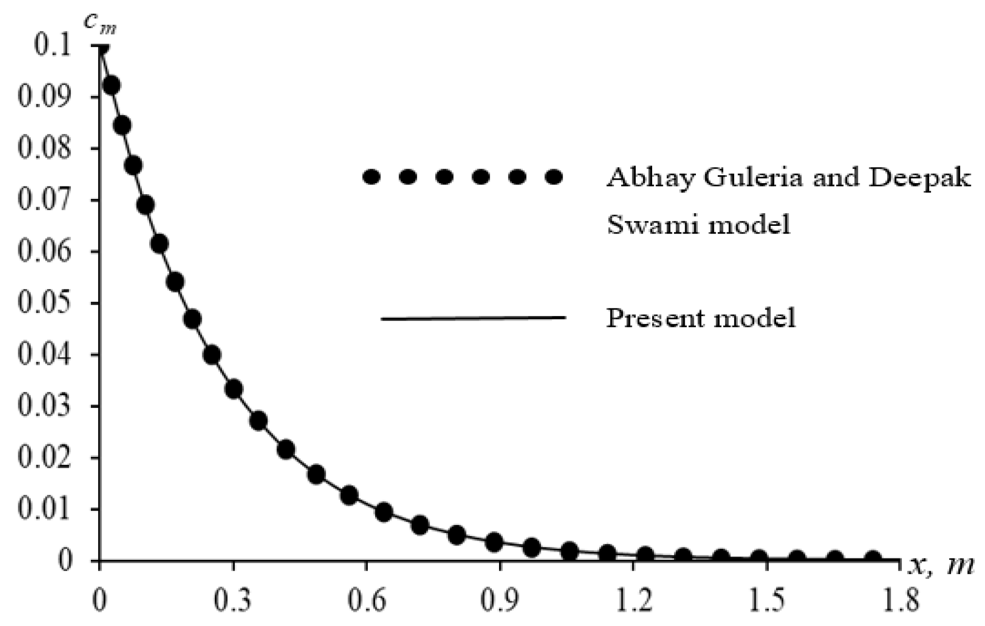
  29. Guleria, A.; Swami, D. Solute Transport Through Saturated Soil Column with Time-Dependent Dispersion. Hydrol. J. 2018, 40, 1–15. [Google Scholar]
  30. Gao, G.; Zhan, H.; Feng, S.; Fu, B.; Ma, Y.; Huang, G. A new mobile-immobile model for reactive solute transport with scale-dependent dispersion. Water Resour. Res. 2010, 46, W08533. [Google Scholar] [CrossRef]
  31. Khuzhayorov, B.; Usmonov, A.; Kholliev, F. Numerical Solution of Anomalous Solute Transport in a Two-Zone Fractal Porous Medium. In APAMCS 2022: Current Problems in Applied Mathematics and Computer Science and Systems; Springer: Cham, Switzerland, 2023; Volume 702, pp. 98–105. [Google Scholar] [CrossRef]
  32. Bear, J. Dynamics of Fluids in Porous Media; Elsevier: New York, NY, USA, 1972. [Google Scholar]
  33. Pickens, J.F.; Grisak, G.E. Modeling of scale-dependent dispersion in hydrogeologic systems. Water Resour. Res. 1981, 17, 1701–1711. [Google Scholar] [CrossRef]
  34. Samarskiy, A.A. Theory of Difference Schemes; Science: Moscow, Russia, 1989; p. 616. [Google Scholar]
  35. Xia, Y.; Wu, J.; Zhou, L. Numerical solution of time-space fractional advection-dispersion equations. Int. Conf. Comput. Exp. Eng. Sci. 2009, 9, 117–126. [Google Scholar]
  36. Khuzhayorov, B.; Usmonov, A.; Nik Long, N.M.A.; Fayziev, B. Anomalous solute transport in a cylindrical two-zone medium with fractal structure. Appl. Sci. 2020, 10, 5349. [Google Scholar] [CrossRef]
  37. Li, G.S.; Sun, C.L.; Jia, X.Z.; Du, D.H. Numerical solution to the multi-term time fractional diffusion equation in a finite domain. Numer. Math. Theory Methods Appl. 2016, 9, 337–357. [Google Scholar] [CrossRef]
Figure 1. Scheme of the solute transport in two-zone medium.
Computation 11 00229 g001
Figure 2. Concentration profile for solute transport at time T = 3600.
Computation 11 00229 g002
Figure 3. Concentration profiles (a): c m at α = 1 , β = 1 ; (b): c m at α = 1 , β = 0.9 ; (c) c i m at α = 1 , β = 1 (d) c i m at α = 1 , β = 0.9 , t = 3600 . Constant: Computation 11 00229 i001, Linear: Computation 11 00229 i002, Exponential: Computation 11 00229 i003.
Computation 11 00229 g003
Figure 4. Concentration profiles (a): c m , (b): c i m at α = 1 , t = 3600 . β = 0.8 : Computation 11 00229 i001, β = 0.9 : Computation 11 00229 i002, β = 1.0 : Computation 11 00229 i003.
Computation 11 00229 g004
Figure 5. Concentration profiles (a): c m , (b): c i m at α = 0.8 , t = 3600 . β = 0.8 : Computation 11 00229 i001, β = 0.9 : Computation 11 00229 i002, β = 1.0 : Computation 11 00229 i003.
Computation 11 00229 g005
Figure 6. Concentration profiles (a): c m , (b): c i m at β = 1 , t = 3600 . α = 0.8 : Computation 11 00229 i001, α = 0.9 : Computation 11 00229 i002, α = 1.0 : Computation 11 00229 i003.
Computation 11 00229 g006
Figure 7. Concentration profiles (a): c m , (b): c i m at β = 0.8 , t = 3600 . α = 0.8 : Computation 11 00229 i001, α = 0.9 : Computation 11 00229 i002, α = 1.0 : Computation 11 00229 i003.
Computation 11 00229 g007
Figure 8. Concentration profiles (a): c m , (b): c i m at α = 1 , t = 3600 . β = 0.8 : Computation 11 00229 i001, β = 0.9 : Computation 11 00229 i002, β = 1.0 : Computation 11 00229 i003.
Computation 11 00229 g008
Figure 9. Concentration profiles (a): c m , (b): c i m at α = 0.8 , t = 3600 . β = 0.8 : Computation 11 00229 i001, β = 0.9 : Computation 11 00229 i002, β = 1.0 : Computation 11 00229 i003.
Computation 11 00229 g009
Figure 10. Concentration profiles (a): c m , (b): c i m at β = 1 , t = 3600 . α = 0.8 : Computation 11 00229 i001, α = 0.9 : Computation 11 00229 i002, α = 1.0 : Computation 11 00229 i003.
Computation 11 00229 g010
Figure 11. Concentration profiles (a): c m , (b): c i m at β = 0.8 , t = 3600 . α = 0.8 : Computation 11 00229 i001, α = 0.9 : Computation 11 00229 i002, α = 1.0 : Computation 11 00229 i003.
Computation 11 00229 g011
Figure 12. Concentration profiles (a): c m , (b): c i m at α = 1 , t = 3600 . β = 0.8 : Computation 11 00229 i001, β = 0.9 : Computation 11 00229 i002, β = 1.0 : Computation 11 00229 i003.
Computation 11 00229 g012
Figure 13. Concentration profiles (a): c m , (b): c i m at α = 0.8 , t = 3600   s . β = 0.8 : Computation 11 00229 i001, β = 0.9 : Computation 11 00229 i002, β = 1.0 : Computation 11 00229 i003.
Computation 11 00229 g013
Figure 14. Concentration profiles (a): c m , (b): c i m at β = 1 , t = 3600   s . α = 0.8 : Computation 11 00229 i001, α = 0.9 : Computation 11 00229 i002, α = 1.0 : Computation 11 00229 i003.
Computation 11 00229 g014
Figure 15. Concentration profiles (a): c m , (b): c i m at β = 0.8 , t = 3600   s . α = 0.8 : Computation 11 00229 i001, α = 0.9 : Computation 11 00229 i002, α = 1.0 : Computation 11 00229 i003.
Computation 11 00229 g015
Figure 16. Concentration profiles c m (ac), c i m (df) at α = 1 , β = 0.9 , t = 3600   s . (a,d): Constant, (b,e): Linear, (c,f): Exponential, k d = 10 4 : Computation 11 00229 i001, 10 3 : Computation 11 00229 i002, 10 2 : Computation 11 00229 i003.
Computation 11 00229 g016
Figure 17. Concentration profiles c m (ac), c i m (df) at α = 1 , β = 1 , t = 3600   s . (a,d): Constant, (b,e): Linear, (c,f): Exponential, k d = 10 4 : Computation 11 00229 i001, 10 3 : Computation 11 00229 i002, 10 2 : Computation 11 00229 i003.
Computation 11 00229 g017aComputation 11 00229 g017b
Figure 18. Concentration profiles c m (ac), c i m (df) at α = 1 , β = 1 , t = 3600 . (a,d): k d = 10 4 , (b,e): k d = 10 3 , (c,f): k d = 10 2 , Constant: Computation 11 00229 i001, Linear: Computation 11 00229 i002, Exponential: Computation 11 00229 i003.
Computation 11 00229 g018aComputation 11 00229 g018b
Disclaimer/Publisher’s Note: The statements, opinions and data contained in all publications are solely those of the individual author(s) and contributor(s) and not of MDPI and/or the editor(s). MDPI and/or the editor(s) disclaim responsibility for any injury to people or property resulting from any ideas, methods, instructions or products referred to in the content.

