Lightweight Implicit Blur Kernel Estimation Network for Blind Image Super-Resolution

Abstract

Blind image super-resolution (Blind-SR) is the process of leveraging a low-resolution (LR) image, with unknown degradation, to generate its high-resolution (HR) version. Most of the existing blind SR techniques use a degradation estimator network to explicitly estimate the blur kernel to guide the SR network with the supervision of ground truth (GT) kernels. To solve this issue, it is necessary to design an implicit estimator network that can extract discriminative blur kernel representation without relying on the supervision of ground-truth blur kernels. We design a lightweight approach for blind super-resolution (Blind-SR) that estimates the blur kernel and restores the HR image based on a deep convolutional neural network (CNN) and a deep super-resolution residual convolutional generative adversarial network. Since the blur kernel for blind image SR is unknown, following the image formation model of blind super-resolution problem, we firstly introduce a neural network-based model to estimate the blur kernel. This is achieved by (i) a Super Resolver that, from a low-resolution input, generates the corresponding SR image; and (ii) an Estimator Network generating the blur kernel from the input datum. The output of both models is used in a novel loss formulation. The proposed network is end-to-end trainable. The methodology proposed is substantiated by both quantitative and qualitative experiments. Results on benchmarks demonstrate that our computationally efficient approach (12x fewer parameters than the state-of-the-art models) performs favorably with respect to existing approaches and can be used on devices with limited computational capabilities.

1. Introduction

The goal of single image super-resolution (SISR) is to generate a high-resolution (HR) image from a low-resolution (LR) one. It has several applications in visual inspection, satellite imaging, medical imaging [1], astronomy, microscope imaging, seismology, remote sensing [2,3], surveillance [4,5,6], biometrics [7], image compression, etc. Most existing literature (e.g., Refs. [8,9,10]) applies a bicubic downsampling kernel to an HR image to generate its LR counterpart such that the inverse process can be modeled. However, the downsampling process is not so unique in real-world LR images. As a result, modeling it may yield very different performances due to the mismatch with the real degradation settings. To overcome such limitations, blind super-resolution (Blind-SR) methods are introduced with the following degradation process:

$$\mathbf{Y}=(\mathbf{k}⊛\widehat{x}){\downarrow }_S+\eta$$

(1)

where $\widehat{x}$ and $\mathbf{Y}$ are the HR and LR images, ⊛ is the convolution operation, $\mathbf{k}$ is the blur kernel, and $\eta$ is the additive white Gaussian noise. ${\downarrow }_S$ is a down-sampling operator with scale factor S. In the real world, $\eta$ also includes factors that can alter the image acquisition process, including inherent sensor noise, stochastic noise, compression artifacts, and possible mismatches between the forward observation model and the camera device.

The approaches that assume a known blur kernel k are named non-blind image SR (Non-Blind-SR see Figure 1a) and have been extensively studied in literature [8,11,12,13,14]. Methods that assume the blur kernel k as unknown are named blind image SR (Blind-SR). Because there exist infinite pairs of SR images and blur kernels can produce the same LR image $\mathbf{Y}$, the SISR is an ill-posed problem. Thus, regularization is needed to choose the most likely one.

In recent years, deep neural network-based methods have achieved remarkable results in SISR [15,16]. For Non-Blind-SR, the blur kernel is the bicubic interpolation kernel [8,11,17,18,19]. This is used to synthesize a large scale dataset for model training. Real LR images might have a large disparity with the bicubic-generated ones since blur kernels are often more complex. This pushed the literature to focus on SR in the presence of unknown blur kernels. Several techniques have been proposed to address the Blind-SR problem by first estimating blur kernels using statistical priors (e.g., patch self-similarity [20]) or deep neural networks (e.g., Refs. [21,22]) and then applying traditional SR techniques assuming a known kernel (e.g., Refs. [23,24]).

These techniques work well to restore minor details but perform independent estimates of the blur kernels and HR images. So, if the blur kernel is incorrectly estimated, the subsequent restoration of the HR image will produce artifacts in the restored images (see Section 4 (Experiments) for a few examples). These introduced methods simultaneously estimate the blur kernel and latent HR image. Methods following such an approach [25,26,27] have focused on creating several efficient blur kernel estimation algorithms. After the blur kernels have been estimated, they are fed into deep models to be used as inputs to rectify the intermediate features used for HR restoration. However, it is unclear if such an exploitation process actually removes the blur.

Existing Blind-SR methods suffer from two main issues: (i) they explicitly estimate the blur kernel with the supervision of GT kernel (see Figure 1b) and require a large volume of training data to train deeper/wider (many model parameters) networks, and (ii) because of their numerous network parameters and large memory requirements, they are challenging to implement on devices with limited computational capabilities (e.g., embedded devices, smartphones, etc.).

We introduce a novel blind-SR technique to tackle such issues by means of a lightweight convolutional neural network (CNN) that can estimate the unknown blur kernel k and generate the super-resolved image ($\widehat{x}$) simultaneously (see Figure 1c). We propose two different modules: (i) the Estimator and (ii) the Super Resolver. In this method, the low-resolution input image LR$\left(\tilde{x}\right)$ is exploited by the former to predict a blur kernel k and by the latter to restore the SR image ($\widehat{x}$). The two outputs (i.e., k and $\widehat{x}$) are then combined in a joint loss function that encourages $\widehat{x}$ to be (i) as close as possible to the ground-truth HR datum (ii) while verifying that it is filtered (with $\widehat{x}$) and the down-scaled version matches the LR input. We introduce an end-to-end training methodology to achieve a high-quality image restoration result (see Figure 2).

The main contributions are:

• We introduce a Blind-SR approach that estimates the blur kernel k and the SR image ($\widehat{x}$) simultaneously. The blur kernel is implicitly estimated, hence not requiring the supervision of a ground truth kernel;
• Our proposed network compares favorably with respect to state-of-the-art approaches that have a similar number of learnable parameters;
• We provide an end-to-end architecture for the proposed algorithm and extensively analyze its performance via quantitative and qualitative evaluation on benchmark datasets.

2. Related Work

2.1. Non-Blind SR

Super Resolution is an ill-posed problem, for which creating image priors has proven to be a successful approach in recent years [28,29,30]. Even though these image prior-based algorithms have produced respectable results, they demand solutions to challenging optimization issues. The application of several DNNs has resulted in major advancements in recent years [8,11,13,18,23,31,32,33,34,35]. Most of these algorithms directly learn the mapping from LR to HR images, thus ignoring the difficult optimization process induced by sophisticated image priors. In Ref. [36], authors demonstrated that using feed-forward networks to predict the mapping of LR images to HR images is insufficient. Haris et al. [36] develop a deep back-projection network based on an error feedback mechanism to improve the LR to HR mapping. In Ref. [37], the image model’s formation process is incorporated into a deep CNN model [18], explicitly ensuring that the estimated high-resolution images satisfy the model of the image formation process.

These deep CNN-based algorithms significantly outperform image prior-based methods and reach state-of-the-art results on many benchmarks. However, such methods suppose that the degradation settings with known blur kernels, for example, the Bicubic interpolation [8,31], Gaussian blur [38], or generalized ones [36], which does not hold true in real circumstances because the blur kernels in the real degradation process are usually more sophisticated. As discussed in Ref. [39], exploiting known/predetermined blur kernels yields SR images with noisy artifacts. Differently, we follow a Blind-SR approach.

2.2. Blind-SR

Different Blind-SR methods [20,40,41] have been proposed to recover the HR image from an input LR with an unknown blur kernel. Conventional techniques typically require the estimate of the blur kernel and the latent HR restoration, which are bound by statistical image priors. Michaeli et al. [20] investigate the internal patch recurrence to estimate the blur kernel and latent HR images. Wang et al. [42] developed an effective probabilistic combination model for blind image SR based on a patch-based image synthesis constraint. In Ref. [43], the authors follow the real-world settings for degradation by using an adversarial learning procedure to train the model with pixel-by-pixel supervision from its LR counterpart in the HR domain. Ref. [44] introduces a deep network trained iteratively with a residual learning method that takes advantage of powerful image regularization and large-scale optimization techniques. Ref. [45] proposes a low-resolution to high-resolution domain translation approach for real-image super-resolution. In Ref. [46], a burst photography pipeline is used to restore the HR.

Despite having achieved reasonable results, these techniques frequently involve complex optimization techniques. To address the Blind-SR problem, multiple approaches develop deep CNNs instead of statistical image priors. In order to estimate blur kernels from LR images, Bell-Kligler et al. [21] develop an effective technique based on an image-specific Internal-GAN. This method provided respectable results and can be used with image SR techniques that rely on blur kernels for performance enhancement, such as those found in Ref. [24]. However, results with considerable artifacts will be produced as a result of the blur kernel errors. For accurate kernel estimation and SR refinement, Gu et al. [22] introduced a spatial feature transform (SFT) and an iterative kernel correction (IKC) technique. Luo et al. [47] estimate the reduced kernel and restore the HR image iteratively in an end-to-end fashion. Our approach has the same spirit as Refs. [22,47] with some relevant differences. In Refs. [22,47] the basic properties of the blind image SR problem are not adequately modeled by separately estimating the blur kernels and latent HR images, thus affecting the final latent HR image restoration. In addition, both such methods are extremely time-consuming and computationally very expensive. Differently, our approach employs a trainable end-to-end network with a limited number of parameters, thus opening to memory and computationally constrained devices.

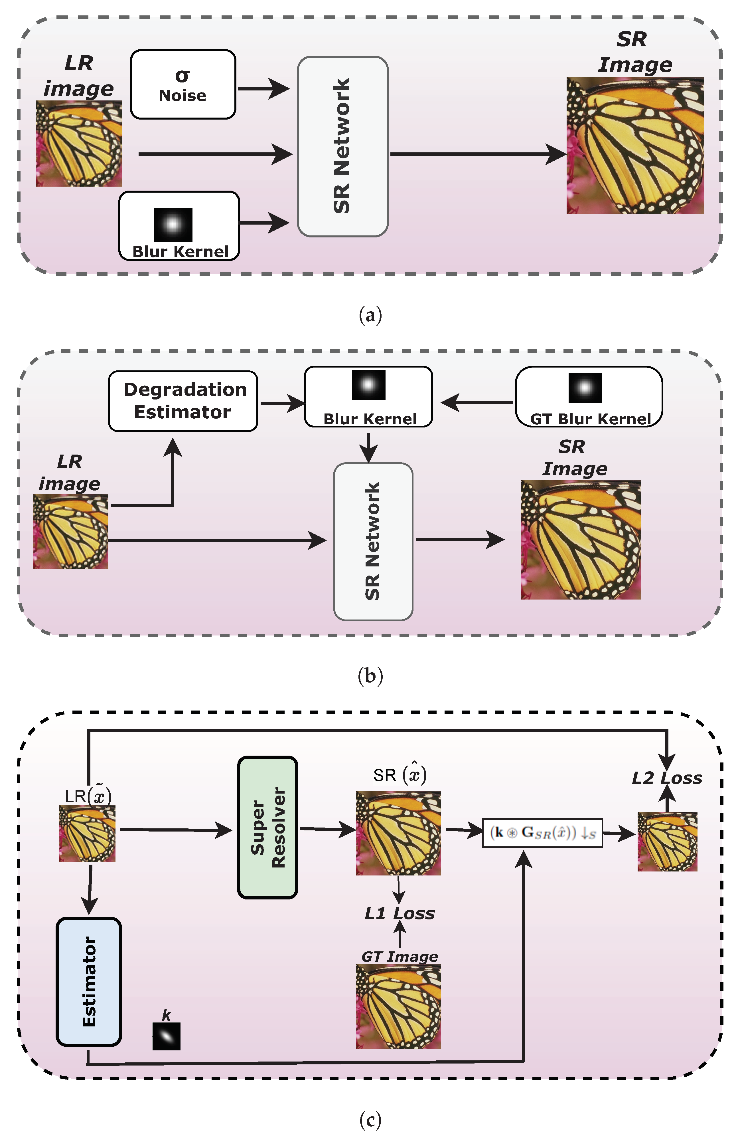
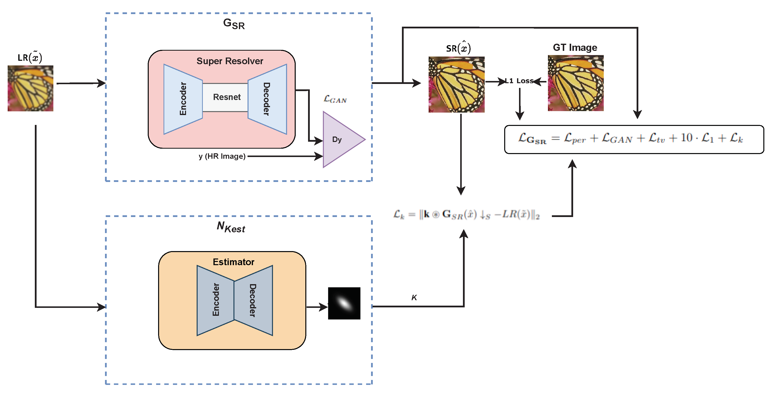
3. Method

3.1. Problem Formulation

According to (1), estimating $\widehat{x}$ from $\mathbf{Y}$ is primarily based on the variational strategy for combining observation and prior knowledge. This requires solving the following minimization problem:

$$\widehat{E}\left(\widehat{x}\right)=arg\underset{\widehat{x}}{min}\frac{1}{2}{\parallel \mathbf{Y}-\mathbf{k}\widehat{x}\parallel }_2^2+\lambda R_W\left(\widehat{x}\right)$$

(2)

where $\frac{1}{2}{\parallel \mathbf{Y}-\mathbf{k}\widehat{x}\parallel }_2^2$ is the data fidelity term related to the model likelihood. It measures how closely the solution matches the observations. $R\left(\widehat{x}\right)$ is a regularization term related to image priors, and $\lambda$ is a trade-off parameter that controls how closely the solution resembles the observations. It is interesting to note that the variational technique directly relates to the Bayesian approach. The generated solutions can be categorized as either maximum a posteriori (MAP) estimates [48,49] or penalized maximum likelihood estimates. Due to strong prior capabilities, we adopt the generator network [43] for super-resolution learning and a simple CNN-based novel kernel estimator network, which predicts the kernel as closest to the original one. We trained both networks end-to-end by exploiting a GAN framework to minimize the energy-based objective function (2) with the discriminative and residual learning approaches, considering the estimated kernel.

3.2. Kernel Estimation

For training kernel estimation network ($N_{kest}$), we provided low-resolution input $\tilde{x}$, which is exploited by the network ($N_{kest}$) and predicts the kernel $\mathbf{k}$, which is further utilized for super resolver learning, as shown in Figure 2.

3.3. Super Resolver

The estimated blur kernel through the kernel estimator network is shown in Figure 2. In the training process, we use the same low-resolution input $\tilde{x}$ for super-resolver $G_{SR}$ and our proposed estimator $N_{kest}$. The super-resolved image $\widehat{x}$ obtained from super-resolver $G_{SR}$ is convolved with the predicted blur kernel $\mathbf{k}$ obtained from the $N_{kest}$ (estimator). The blur kernel $\mathbf{k}$ predicted by $N_{kest}$ (estimator)is used to calculate the novel loss ${\mathcal{L}}_k$ after the convolution with the super-resolved image. We calculate the ${\mathcal{L}}_1$ from the super-resolved image $\widehat{x}$ and ground truth. The loss ${\mathcal{L}}_k$ is added to the ${\mathcal{L}}_1$ and other network losses (i.e., ${\mathcal{L}}_{per},{\mathcal{L}}_{GAN},{\mathcal{L}}_{tv}$) to calculate the final loss ${\mathcal{L}}_{{\mathbf{G}}_{\mathbf{SR}}}$ as given in (9).

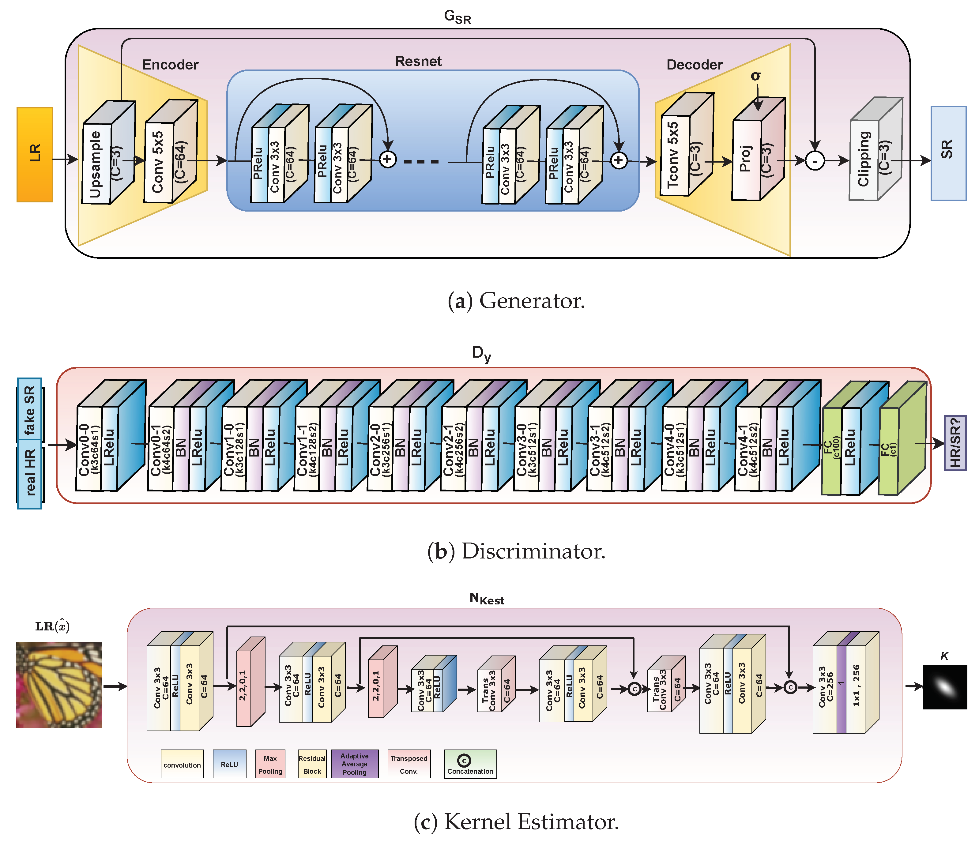
3.4. Network Architectures

The network architectures of the Generator (${\mathbf{G}}_{SR}$), Discriminator (${\mathbf{D}}_y$), and Kernel Estimator (${\mathbf{N}}_{kest}$) are depicted in Figure 3. The letters s, c, and k denoted stride size, number of filters, and kernel size, respectively.

3.4.1. Generator Network (${\mathbf{G}}_{SR}$):

As illustrated in Figure 3a, the Encoder and Decoder include 64 feature maps, $C\times H\times W$ tensors, a $5\times 5$ kernel, and C input channels. The LR input $\tilde{x}$ is upsampled using Bilinear kernel ${\mathbf{H}}^{\mathrm{T}}$. There are 5 residual blocks, 2 pre-activation convolutional layers with 64 feature maps each, and $3\times 3$ kernel. Pre-activations are parametrized rectified linear units (PReLU) that support 64 feature maps. The project layer (Proj) [50] in the decoder determines the proximal map using standard deviation ($\sigma$), which accounts for the prior terms and data fidelity term. The $\alpha$ parameter in Proj is fine-tuned with the back-propagation in training. In addition, the Resnet block located in-between the encoder and the decoder is where the noise is estimated. The input LR image is then subtracted from the estimated residual image provided by the Decoder. Finally, the clipping layer is responsible for complying with the valid intensity of the image ranging from 0 to 255. In training, reflection padding is utilized to lag the convolutional layers, which makes the consistent change in the input image.

3.4.2. Discriminator Network (${\mathbf{D}}_y$):

Figure 3b shows the discriminator network architecture. This aims to classify if the input is a generated SR image $\widehat{x}$ (i.e., fake) or a real HR image y. The discriminator comprises $3\times 3$ kernel, $4\times 4$ kernel, 64 feature map, 512 feature map, leaky ReLU, and Batch Normalization (BN) as suggested in SRGAN [23].

3.4.3. Estimator Network (${\mathbf{N}}_{kest}$):

Estimating the blur kernels from given LR images is difficult because blur and downsampling operations result in information loss. Existing methods typically require sophisticated priors and the solution of complex optimization problems [20]. Bell-Kligler et al. estimate the blur kernel from a single LR image using a generative adversarial network in Ref. [21]. Unlike [20,21], we develop a simple deep CNN model (${\mathbf{N}}_{kest}$) that ingests an LR image to estimate its blur kernel. This network, shown in Figure 3c, is trained using (8).

3.5. Loss Calculation

3.5.1. Texture Loss (${\mathcal{L}}_{GAN}$):

Although perceptual loss can improve the overall quality of a reconstructed image, it still introduces unwanted high-frequency components. That is why we consider including texture loss in the total loss function as follows.

$$\begin{array}{cc}\hfill {\mathcal{L}}_{GAN}=& {\mathcal{L}}_{RaGAN}-{\mathbb{E}}_y[log(1-{\mathbf{D}}_{\mathbf{y}})(\mathbf{y},{\mathbf{G}}_{\mathbf{SR}}(\widehat{\left(x\right)}))]\hfill \\ \hfill -& {\mathbb{E}}_{\widehat{y}}[log\left({\mathbf{D}}_{\mathbf{y}}({\mathbf{G}}_{SR}\left(\widehat{x}\right),y)\right)]\hfill \end{array}$$

(3)

where ${\mathbb{E}}_y$ and ${\mathbb{E}}_{\widehat{y}}$ are used for the average of real (y) and fake ($\widehat{y}$) data, respectively. We use a discriminator that gives the GAN score of a real image (HR) and a fake image (SR) as used in Ref. [10]. It is defined as follows.

$${\mathbf{D}}_y(y,\widehat{y})\left(C\right)=\sigma (C\left(y\right)-\mathbb{E}\left[C\left(\widehat{y}\right)\right]$$

(4)

The sigmoid function and the output of the raw discriminator have been represented by $\sigma$ and C, respectively, as shown in Figure 3b.

3.5.2. Perceptual Loss (${\mathcal{L}}_{per}$):

To generate images with more precise brightness and realistic textures, (${\mathcal{L}}_{per}$) based on the VGG network, it is configured to use information from the feature layer before the activation layer. On the activation layer of the pre-trained deep neural network, it is specified to minimize the Euclidean distance between two activation features.

$$\begin{array}{cc}\hfill {\mathcal{L}}_{per}=& \frac{1}{N}\sum _i^N{\mathcal{L}}_{VGG}\hfill \\ \hfill =& \frac{1}{N}\sum _i^N\parallel \varphi ({\mathbf{G}}_{SR}\left(\widehat{x_i}\right)-\varphi \left(y_i\right){\parallel }_1\hfill \end{array}$$

(5)

where $\varphi$ denotes extracted feature from VGG-19 pretrained network as specified in Ref. [10].

3.5.3. TV (Total-Variation) Loss (${\mathcal{L}}_{tv}$):

The absolute differences between adjacent pixel values in the input images are added to determine total variation loss. Total Variation loss measures the amount of noise in images. To remove the image’s rough texture and make the resultant image look smoother, we added the total variation loss to the total loss, as follows.

$$\begin{array}{cc}\hfill {\mathcal{L}}_{tv}=& \frac{1}{N}\sum _i^N(\parallel {▿}_h{\mathbf{G}}_{SR}\left({\widehat{x}}_i\right)-{▿}_h\left(y_i\right){\parallel }_1\hfill \\ \hfill +& \parallel {▿}_v{\mathbf{G}}_{SR}\left({\widehat{x}}_i\right)-{▿}_v\left(y_i\right){\parallel }_1)\hfill \end{array}$$

(6)

where ${▿}_v$ and ${▿}_h$ represent the vertical and horizontal gradients of the images.

3.5.4. Content Loss (${\mathcal{L}}_1$)

Mean Absolute Error (MAE) loss is used as the model’s content loss to ensure that low-frequency information is the same between the reconstructed and LR images. Its job is to minimize the difference between the pixels in the generated HR images and those in the real HR images. By making the distance between pixels smaller, the accuracy of the reconstructed image information can be evaluated more quickly and accurately, leading to a higher peak signal-to-noise ratio. We incorporated content loss to a total loss to generate a good quality reconstructed image, as follows.

$${\mathcal{L}}_1=\frac{1}{N}\sum _i^N{\parallel {\mathbf{G}}_{SR}\left(\widehat{x}\right)-y_i\parallel }_1$$

(7)

where N represents the batch size.

3.5.5. Estimator Loss(${\mathcal{L}}_k)$:

We computed the estimator loss in such a manner that we combined two outputs (i.e., k and $\widehat{x}$) such that $\widehat{x}$ should be as close as possible to the ground-truth HR image, and it is convolved (with $\widehat{x}$) and the down-scaled version matches the LR input.

$${\mathcal{L}}_k=\parallel \mathbf{k}⊛{\mathbf{G}}_{SR}\left(\widehat{x}\right){{\downarrow }_S-LR\left(\tilde{x}\right)\parallel }_2$$

(8)

where S is a downscaling factor, k is the estimated kernel, and ${\mathbf{G}}_{SR}\left(\widehat{x}\right)$ is the super-resolved imaged.

Total loss function (${\mathcal{L}}_{{\mathbf{G}}_{\mathbf{SR}}}$) formulation is defined as:

$${\mathcal{L}}_{{\mathbf{G}}_{\mathbf{SR}}}={\mathcal{L}}_{GAN}+{\mathcal{L}}_{per}+{\mathcal{L}}_{tv}+10·{\mathcal{L}}_1+{\mathcal{L}}_k$$

(9)

4. Experiments

4.1. Datasets

We followed a common protocol [22,43,45,47] and used 3450 high-resolution (HR) images from DIV2K [51] and Flickr2K [52] for model training. For a fair comparison with existing approaches, we followed [22,47] and trained/evaluated our approach with the two following degradation settings.

4.1.1. Setting 1

We follow the protocol in Ref. [22] and set the kernel size to 21. For scale factors 4 and 2, the kernel width is uniformly sampled during training in the ranges of [0.2, 4.0] and [0.2, 2.0]. Evaluation is conducted on popular benchmark HR datasets, such as Set5 [53], Set14 [54], Urban100 [55], BSD100 [56], and Manga109 [57]. For a fair comparison with existing methods, during testing, we adopted the same approach of Ref. [22] and uniformly selected 8 kernels from the ranges [1.8, 3.2] and [0.80, 1.60] for scale factors 4 and 2, respectively. The HR images are first blurred using the selected blur kernels, then downsampled to generate synthetic test images.

4.1.2. Setting 2

Following the training protocol of Ref. [47], we set the kernel size to 11 and generated Anisotropic Gaussian kernels with both axes’ lengths randomly taken in the range (0.6, 5). A random rotation in $[-\pi ,\pi ]$ is then applied. We added uniform multiplicative noise (up to 25 % of each kernel pixel value) and normalized it, to sum up to one. For a fair comparison, the evaluation is run on the DIV2KRK benchmark dataset (with no additional blur kernel applied to the images since these are already degraded).

4.2. Model Optimization

We trained our model with $32\times 32$ LR patches for 51,000 iterations. To minimize (9), we used 16 samples per batch with the Adam optimizer [58] having ${\beta }_1=0.9$, ${\beta }_2=0.999$, and $ϵ={10}^{-8}$ without weight decay for both generator and discriminator. We initially set the learning rate to ${10}^{-4}$, then reduce it by a factor of 2 after 5 K, 10 K, 20 K, and 30 K iterations. The projection layer parameter $\sigma$ (standard deviation) is estimated according to Ref. [59] from the input LR image. We initialize the projection layer parameter $\alpha$ on log-scale values from ${\alpha }_{max}$ = 2 to ${\alpha }_{min}=1$ and then further fine-tune during the training via a back-propagation. Using a GAN framework in Ref. [60] and the following loss functions, we fine-tune the SRResCGAN network to learn the super-resolution. (i.e., pre-trained ${\mathbf{G}}_{SR}$) [43].

Random vertical and horizontal flipping and $90deg$ rotations are used as data augmentation strategies.

4.3. Technical Details

We used Pytorch to implement our technique. The experiments use an i7-8700H processor, 32 GB of RAM, and a 24 GB NVIDIA GeForce RTX 3090 GPU on Ubuntu 20.04 LTS. It took approximately 18.5 h to train the model.

4.4. Evaluation Metrics

For a fair comparison, we evaluated the trained model under the Peak Signal-to-Noise Ratio (PSNR) and Structural Similarity (SSIM) [61] metrics. The PSNR and SSIM are distortion-based measures. The RGB color space is used to evaluate the quantitative SR results.

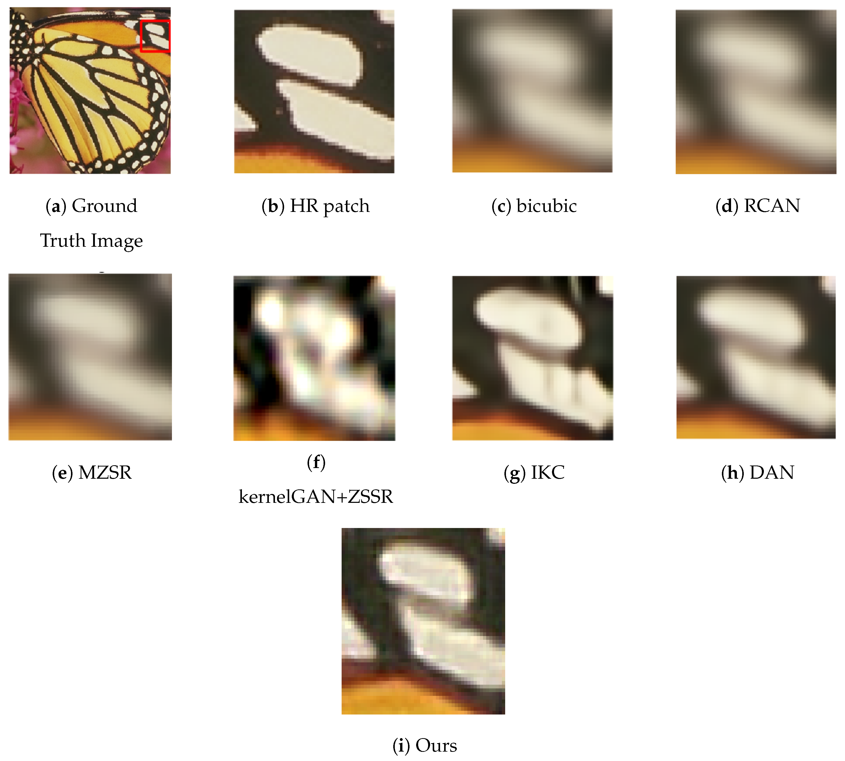
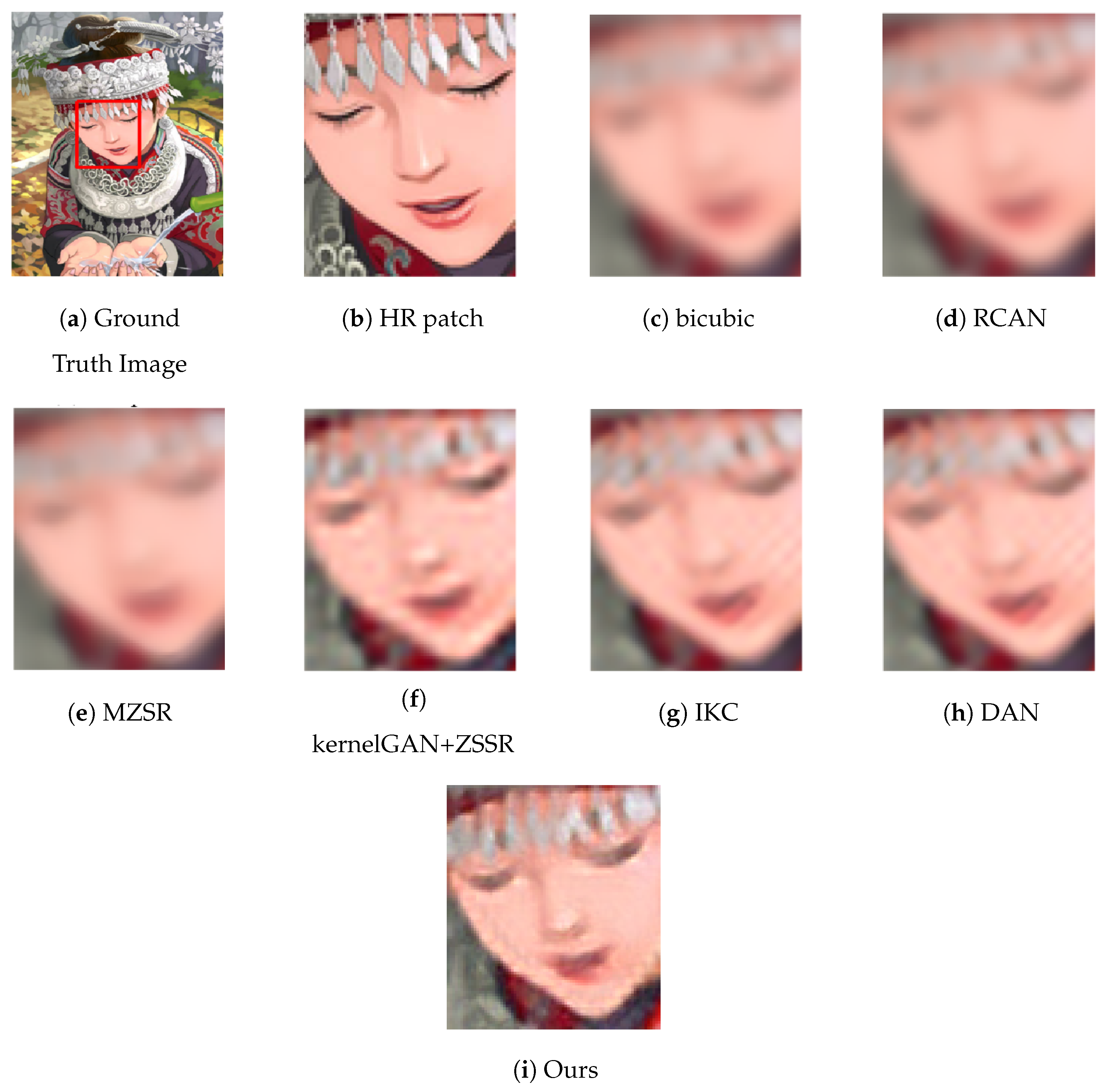
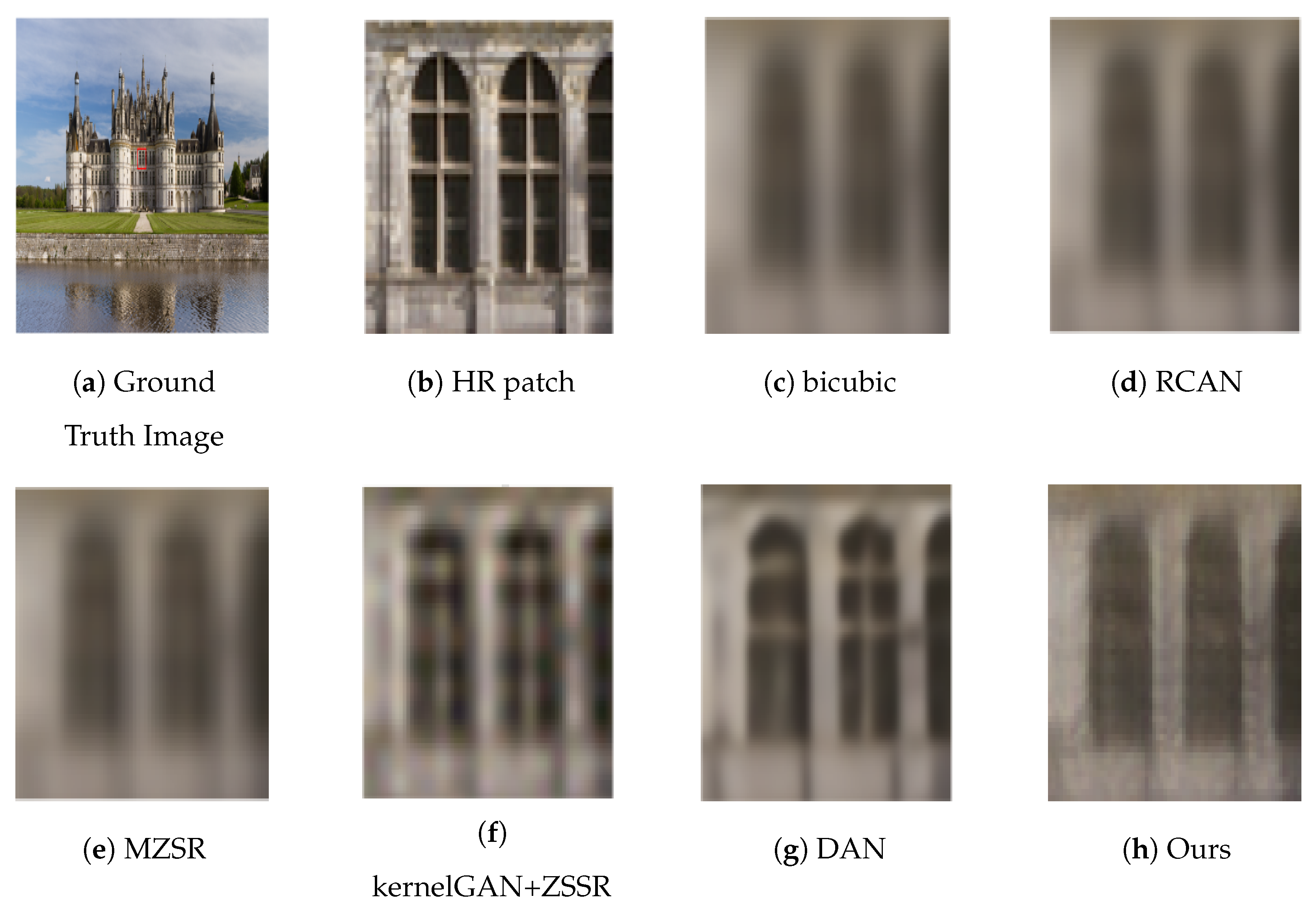
4.5. Experimental Results

4.5.1. Setting 1

We compare the proposed method with state-of-the-art Blind-SR approaches such as IKC [22], DAN [47], and KernelGAN [21] (which explicitly estimates the blur kernels), as well as with blind deblurring methods such as Pan et al [62]. We also compare our results with existing Non-Blind-SR approaches like RCAN [11], ZSSR [24], CARN [17], and MZSR [63].

Table 1. Comparing state-of-the-art Non-Blind (*) and Blind-SR techniques under Setting 1.

Methods	Scale	Set5 PSNR/SSIM	Set14 PSNR/SSIM	B100 PSNR/SSIM	Urban100 PSNR/SSIM	Manga109 PSNR/SSIM	#Params (M)
Bicubic		28.65/0.84	26.70/0.77	26.26/0.73	23.61/0.74	25.73/0.84	/
RCAN * [11]		29.73/0.86	27.65/0.79	27.07/0.77	24.74/0.78	27.64/0.87	15.59
ZSSR * [24]		29.74/0.86	27.57/0.79	26.96/0.76	24.34/0.77	27.10/0.87	0.22
MZSR * [63]		29.88/0.86	27.32/0.79	26.96/0.77	24.12/0.77	27.24/0.87	0.22
CARN * [17]	×2	30.99/0.87	28.10/0.78	26.78/0.72	25.77/0.76	26.86/0.86	1.592
Pan et al. [62] + CARN [17]		24.20/0.74	21.12/0.61	22.69/0.64	18.59/0.58	21.54/0.74	/
CARN [17] + Pan et al. [62]		31.27/0.89	29.03/0.82	28.72/0.80	25.62/0.79	29.58/0.91	/
KernelGAN [21] + ZSSR [24]		26.02/0.77	20.19/0.58	21.42/0.60	19.55/0.61	24.22/0.78	0.52
KernelGAN [21] + MZSR [63]		29.39/0.88	23.94/0.72	24.42/0.73	23.39/0.77	28.38/0.89	0.52
IKC [22]		33.62/0.91	29.14/0.85	28.46/0.82	26.59/0.84	30.51/0.91	9.05
DAN [47]		34.55/0.92	29.92/0.86	29.66/0.85	27.96/0.87	33.82/0.95	4.33
Ours		31.02/0.89	27.87/0.80	27.67/0.79	25.11/0.80	28.44/0.89	0.38
Bicubic		24.49/0.69	23.01/0.59	23.64/0.59	20.58/0.57	21.97/0.70	/
RCAN * [11]		24.95/0.71	23.33/0.61	23.65/0.62	20.73/0.61	23.30/0.76	15.59
ZSSR * [24]		24.77/0.70	23.32/0.60	23.72/0.61	20.74/0.59	22.75/0.74	0.22
MZSR * [63]		24.99/0.70	23.45/0.61	23.83/0.61	20.92/0.61	23.25/0.76	0.22
CARN * [17]	×4	26.57/0.74	24.62/0.62	24.79/0.59	22.17/0.58	21.85/0.68	1.592
Pan et al. [62]+ CARN [17]		18.10/0.48	16.59/0.39	18.46/0.44	15.47/0.38	16.78/0.53	/
CARN [17]+Pan et al. [62]		28.69/0.80	26.40/0.69	26.10/0.65	23.46/0.65	25.84/0.80	/
KernelGAN [21] + ZSSR [24]		17.59/0.42	19.20/0.49	17.14/0.40	16.95/0.47	19.40/0.61	0.52
KernelGAN [21] + MZSR [63]		23.08/0.66	22.24/0.61	21.51/0.56	19.37/0.58	22.05/0.70	0.52
IKC [22]		27.84/0.80	25.02/0.67	24.76/0.65	22.41/0.67	25.37/0.81	9.05
DAN [47]		27.64/0.80	25.46/0.69	25.35/0.67	23.21/0.71	27.04/0.85	4.33
Ours		25.94/0.73	23.83/0.62	24.12/0.60	21.15/0.59	22.15/0.71	0.38

shows the quantitative evaluation of the benchmark datasets on scale factors ×2 and ×4. The results show that the proposed method performed better than most of the considered methods. IKC [22] and DAN [47] have higher PSNRs and SSIMs but require a large number of parameters as compared to our method. Figure 4 and Figure 5 show visualized SR results of the evaluated methods when scaled by a factor of ×4, and the blur kernel in the degradation model is an isotropic Gaussian blur kernel. The non-blind SR approaches, such as Bicubic, RCAN [11], and MZSR [63], produce results with a considerable blur impact because they do not mimic the blur kernels while super-resolving LR images (Figure 4c–e). The KernelGAN [21] approach proposes an effective blur kernel estimation method and can use existing non-blind SR methods for blind SR, such as ZSSR [24]. However, because blur kernel estimate and HR image restoration are distinct processes, HR image restoration cannot rectify problems produced by inaccurate blur kernels. As a result, the restored image has artifacts, as illustrated in Figure 5f.

The IKC [22] proposed an effective iterative kernel correction method to explicitly estimate blur kernels and restore sharp images, as shown in Figure 4g, but has a large number of parameters.

Figure 4h shows that the state-of-the-art blind SR method DAN [47] also produce visually fine results.

On the other hand, our proposed method implicitly estimates blur kernels and HR images simultaneously using a lightweight (less number of parameters) end-to-end trainable network and the super resolver network to restore the HR images. Figure 4 and Figure 5 show that our generated SR images are much better than state-of-the-art methods (e.g., Figure 4d–f), however Figure 4g,h outperforms ours.

4.5.2. Setting 2

Setting 2 used irregular blur kernels (anisotropic), which is more generic but harder to solve.

Table 2. Comparing state-of-the-art Non-Blind (*) and Blind-SR techniques under Setting 2.

Scale	Bicubic	RCAN* [11]	ZSSR* [24]	KernelGAN [21] + ZSSR [24]	IKC [22]	DAN [47]	KOALAnet [27]	Ours
×2	27.00/0.77	27.52/0.79	27.47/0.79	27.62/0.79	29.24/0.84	31.09/0.88	30.48/0.86	27.53/0.79
×4	23.89/0.64	24.16/0.65	24.11/0.65	24.50/0.66	25.26/0.70	26.42/0.73	26.23/0.72	24.67/0.66

shows that our proposed method performs favorably against some state-of-the-art methods like RCAN [11], ZSSR [24], but IKC [22], DAN [47], and KOALAnet [27] have better results since they explicit estimate the blur kernels (hence assuming a GT kernel is available) and have a large number of parameters. Figure 6 shows the visual comparison with the state-of-the-art (SOTA) super-resolution (SR) method with setting 2.

4.6. Computational Cost

In

Table 3. Comparison of FLOPs.

Methods	FLOPs
IKC [22]	2178.72 G
DAN [47]	929.35 G
Ours	295.17 G

we report on the number of FLOPs required to run our method and compare it against [22] and [47]. We followed the same methodology described in Ref. [47] and computed the FLOPs and inference time considering an input size of $270\times 180$. This is done for 40 images synthesized by 8 blur kernels from the Set5 dataset. Results show that, with $3\times$ less required FLOPs, our model achieves a significantly faster inference time yielding 0.243 s/image while DAN and IKC have 0.312 and 1.735 s/image, respectively.

4.7. Ablation Study

In

Table 4. This table displays that the DIV2K validation set (100 images with unknown blur kernels) was used for our ablation investigation.

Methods	w/o (${\mathit{N}}_{\mathbf{kest}}$)	Ours
PSNR/SSIM	25.63/0.69	25.80/0.71

, we analyze the impact of the kernel estimation module. Results are computed on the DIV2K validation set with unknown blur kernels. It shows that without using (${\mathbf{N}}_{kest}$) it does not generate good SR images in terms of PSNR/SSIM, and with our proposed method, PSNR/SSIM increased by +0.17/+0.02, respectively. To study the effects of different blur kernels, we compute the results in

Table 5. Quantitative performance of proposed approach on Set5(×4) with different blur kernels width.

Kernel Width	1.0	2.5	3.0	3.5	4.0
Bicubic	25.20/0.72	24.38/0.69	23.70/0.66	23.18/0.63	22.80/0.62
ZSSR [24]	26.30/0.76	25.06/0.72	24.11/0.68	23.44/0.65	22.95/0.62
IKC [22]	28.12/0.82	28.32/0.82	28.29/0.81	27.90/0.80	24.26/0.69
Ours	26.31/0.76	26.05/0.73	25.09/0.70	24.17/0.66	23.38/0.63

. These indicate that our method can generalize better than a Non-Blind-SR method (i.e., Ref. [24]) while maintaining competitive performance with a Blind-SR method (i.e., Ref. [22]) requiring $7.5\times$ more learnable parameters.

5. Conclusions

In this paper, we have introduced an effective, lightweight, and implicit blur kernel estimation end-to-end approach for blind image super-resolution (blind-SR). Our proposed approach is based on a deep convolutional neural network (CNN) named estimator and a deep super-resolution residual convolutional generative adversarial network named super resolver. The Estimator module implicitly estimates the blur kernels from the LR input without the supervision of the ground truth kernel. The Super Resolver module restores the SR image by exploiting a GAN framework to minimize the energy-based objective function with the discriminative and residual learning approaches, considering the estimated kernel. The whole architecture is trained in an end-to-end fashion. Results on different benchmark datasets show that our approach achieves better performance than state-of-the-art methods having a similar number of learnable parameters, enabling it to work on devices with limited computational capacity.

References

- Dunnhofer, M.; Martinel, N.; Micheloni, C. Improving MRI-based Knee Disorder Diagnosis with Pyramidal Feature Details. In Proceedings of Machine Learning Research, Proceedings of the Fourth Conference on Medical Imaging with Deep Learning, Lubeck, Germany, 7–9 July 2021; Heinrich, M., Dou, Q., de Bruijne, M., Lellmann, J., Schläfer, A., Ernst, F., Eds.; PMLR: New York, NY, USA, 2021; Volume 143, pp. 131–147. [Google Scholar]
- Huang, S.; Teo, R.; Leong, W.; Martinel, N.; Foresti, G.L.; Micheloni, C. Coverage Control of Multiple Unmanned Aerial Vehicles: A Short Review. Unmanned Syst. 2018, 6, 131–144. [Google Scholar] [CrossRef]
- Leong, W.L.; Martinel, N.; Huang, S.; Micheloni, C.; Foresti, G.L.; Teo, R.S.H. An Intelligent Auto-Organizing Aerial Robotic Sensor Network System for Urban Surveillance. J. Intell. Robot. Syst. 2021, 102, 33. [Google Scholar] [CrossRef]
- Martinel, N.; Micheloni, C.; Foresti, G.L. A pool of multiple person re-identification experts. Pattern Recognit. Lett. 2016, 71, 23–30. [Google Scholar] [CrossRef]
- Martinel, N.; Foresti, G.L.; Micheloni, C. Deep Pyramidal Pooling With Attention for Person Re-Identification. IEEE Trans. Image Process. 2020, 29, 7306–7316. [Google Scholar] [CrossRef]
- Martinel, N.; Dunnhofer, M.; Pucci, R.; Foresti, G.L.; Micheloni, C. Lord of the Rings: Hanoi Pooling and Self-Knowledge Distillation for Fast and Accurate Vehicle Reidentification. IEEE Trans. Ind. Inf. 2022, 18, 87–96. [Google Scholar] [CrossRef]
- Bansal, V.; Foresti, G.L.; Martinel, N. Cloth-Changing Person Re-Identification With Self-Attention. In Proceedings of the IEEE/CVF Winter Conference on Applications of Computer Vision (WACV) Workshops, Waikoloa, HI, USA, 4–8 January 2022; pp. 602–610. [Google Scholar]
- Kim, J.; Lee, J.K.; Lee, K.M. Accurate image super-resolution using very deep convolutional networks. In Proceedings of the IEEE CVPR, Las Vegas, NV, USA, 27–30 June 2016; pp. 1646–1654. [Google Scholar]
- Xia, B.; Hang, Y.; Tian, Y.; Yang, W.; Liao, Q.; Zhou, J. Efficient Non-Local Contrastive Attention for Image Super-Resolution. arXiv 2022, arXiv:2201.03794. [Google Scholar] [CrossRef]
- Wang, X.; Yu, K.; Wu, S.; Gu, J.; Liu, Y.; Dong, C.; Qiao, Y.; Change Loy, C. Esrgan: Enhanced super-resolution generative adversarial networks. In Proceedings of the ECCVW, Munich, Germany, 8–14 September 2018. [Google Scholar]
- Zhang, Y.; Li, K.; Li, K.; Wang, L.; Zhong, B.; Fu, Y. Image super-resolution using very deep residual channel attention networks. In Proceedings of the ECCV, Munich, Germany, 8–14 September 2018; pp. 286–301. [Google Scholar]
- Dong, C.; Loy, C.C.; Tang, X. Accelerating the super-resolution convolutional neural network. In Proceedings of the Computer Vision–ECCV 2016: 14th European Conference, Amsterdam, The Netherlands, 11–14 October 2016; Springer: Berlin/Heidelberg, Germany, 2016; pp. 391–407. [Google Scholar]
- Haris, M.; Shakhnarovich, G.; Ukita, N. Deep back-projection networks for super-resolution. In Proceedings of the IEEE Conference on Computer Vision and Pattern Recognition, Salt Lake City, UT, USA, 18–22 June 2018; pp. 1664–1673. [Google Scholar]
- Hu, X.; Mu, H.; Zhang, X.; Wang, Z.; Tan, T.; Sun, J. Meta-SR: A magnification-arbitrary network for super-resolution. In Proceedings of the IEEE/CVF Conference on Computer Vision and Pattern Recognition, Long Beach, CA, USA, 15–20 June 2019; pp. 1575–1584. [Google Scholar]
- Bhat, G.; Danelljan, M.; Timofte, R.; Akita, K.; Cho, W.; Fan, H.; Jia, L.; Kim, D.; Lecouat, B.; Li, Y.; et al. NTIRE 2021 challenge on burst super-resolution: Methods and results. In Proceedings of the IEEE Computer Society Conference on Computer Vision and Pattern Recognition Workshops, Nashville, TN, USA, 19–25 June 2021; pp. 613–626. [Google Scholar] [CrossRef]
- Wei, P.; Lu, H.; Timofte, R.; Lin, L.; Zuo, W.; Pan, Z.; Li, B.; Xi, T.; Fan, Y.; Zhang, G.; et al. AIM 2020 Challenge on Real Image Super-Resolution: Methods and Results; Springer: Cham, Switzerland, 2020; Volume 12537 LNCS, pp. 392–422. [Google Scholar] [CrossRef]
- Ahn, N.; Kang, B.; Sohn, K.A. Fast, accurate, and lightweight super-resolution with cascading residual network. In Proceedings of the ECCV, Munich, Germany, 8–14 September 2018; pp. 252–268. [Google Scholar]
- Lim, B.; Son, S.; Kim, H.; Nah, S.; Mu Lee, K. Enhanced deep residual networks for single image super-resolution. In Proceedings of the IEEE CVPR, Honolulu, HI, USA, 21–26 July 2017; pp. 136–144. [Google Scholar]
- Dai, T.; Cai, J.; Zhang, Y.; Xia, S.T.; Zhang, L. Second-order attention network for single image super-resolution. In Proceedings of the IEEE/CVF CVPR, Long Beach, CA, USA, 15–20 June 2019; pp. 11065–11074. [Google Scholar]
- Michaeli, T.; Irani, M. Nonparametric blind super-resolution. In Proceedings of the IEEE ICCV, Sydney, Australia, 1–8 December 2013; pp. 945–952. [Google Scholar]
- Bell-Kligler, S.; Shocher, A.; Irani, M. Blind super-resolution kernel estimation using an internal-gan. NeurIPS 2019, 32. [Google Scholar] [CrossRef]
- Gu, J.; Lu, H.; Zuo, W.; Dong, C. Blind super-resolution with iterative kernel correction. In Proceedings of the IEEE/CVF CVPR, Long Beach, CA, USA, 15–20 June 2019; pp. 1604–1613. [Google Scholar]
- Ledig, C.; Theis, L.; Huszár, F.; Caballero, J.; Cunningham, A.; Acosta, A.; Aitken, A.; Tejani, A.; Totz, J.; Wang, Z.; et al. Photo-realistic single image super-resolution using a generative adversarial network. In Proceedings of the IEEE CVPR, Honolulu, HI, USA, 21–26 July 2017; pp. 4681–4690. [Google Scholar]
- Shocher, A.; Cohen, N.; Irani, M. “zero-shot” super-resolution using deep internal learning. In Proceedings of the IEEE CVPR, Salt Lake City, UT, USA, 18–22 June 2018; pp. 3118–3126. [Google Scholar]
- Liang, J.; Zhang, K.; Gu, S.; Van Gool, L.; Timofte, R. Flow-based kernel prior with application to blind super-resolution. In Proceedings of the IEEE/CVF CVPR, Nashville, TN, USA, 19–25 June 2021; pp. 10601–10610. [Google Scholar]
- Wang, L.; Wang, Y.; Dong, X.; Xu, Q.; Yang, J.; An, W.; Guo, Y. Unsupervised degradation representation learning for blind super-resolution. In Proceedings of the IEEE/CVF CVPR, Nashville, TN, USA, 19–25 June 2021; pp. 10581–10590. [Google Scholar]
- Kim, S.Y.; Sim, H.; Kim, M. Koalanet: Blind super-resolution using kernel-oriented adaptive local adjustment. In Proceedings of the IEEE/CVF CVPR, Nashville, TN, USA, 19–25 June 2021; pp. 10611–10620. [Google Scholar]
- Glasner, D.; Bagon, S.; Irani, M. Super-resolution from a single image. In Proceedings of the ICCV 2009, Kyoto, Japan, 27 September–4 October 2009; pp. 349–356. [Google Scholar]
- Yang, J.; Wright, J.; Huang, T.; Ma, Y. Image super-resolution as sparse representation of raw image patches. In Proceedings of the IEEE CVPR 2008, Anchorage, AK, USA, 24–26 June 2008; pp. 1–8. [Google Scholar]
- Timofte, R.; De Smet, V.; Van Gool, L. A+: Adjusted anchored neighborhood regression for fast super-resolution. In Proceedings of the ACCV, Santiago, Chile, 7–13 December 2015; Springer: Berlin/Heidelberg, Germany, 2015; pp. 111–126. [Google Scholar]
- Dong, C.; Loy, C.C.; He, K.; Tang, X. Learning a deep convolutional network for image super-resolution. In Proceedings of the ECCV, Zurich, Switzerland, 6–12 September 2014; Springer: Berlin/Heidelberg, Germany, 2014; pp. 184–199. [Google Scholar]
- Kim, J.; Lee, J.K.; Lee, K.M. Deeply-recursive convolutional network for image super-resolution. In Proceedings of the IEEE CVPR, Las Vegas, NV, USA, 27–30 June 2016; pp. 1637–1645. [Google Scholar]
- Tai, Y.; Yang, J.; Liu, X. Image super-resolution via deep recursive residual network. In Proceedings of the IEEE CVPR, Honolulu, HI, USA, 21–26 July 2017; pp. 3147–3155. [Google Scholar]
- Lai, W.S.; Huang, J.B.; Ahuja, N.; Yang, M.H. Deep laplacian pyramid networks for fast and accurate super-resolution. In Proceedings of the IEEE CVPR, Honolulu, HI, USA, 21–26 July 2017; pp. 624–632. [Google Scholar]
- Zhang, Y.; Tian, Y.; Kong, Y.; Zhong, B.; Fu, Y. Residual dense network for image super-resolution. In Proceedings of the IEEE CVPR, Salt Lake City, UT, USA, 18–23 June 2018; pp. 2472–2481. [Google Scholar]
- Zhang, K.; Zuo, W.; Zhang, L. Learning a single convolutional super-resolution network for multiple degradations. In Proceedings of the IEEE CVPR, Salt Lake City, UT, USA, 18–23 June 2018; pp. 3262–3271. [Google Scholar]
- Pan, J.; Liu, Y.; Sun, D.; Ren, J.; Cheng, M.M.; Yang, J.; Tang, J. Image formation model guided deep image super-resolution. In Proceedings of the AAAI Conference on Artificial Intelligence, New York, NY, USA, 7–12 February 2020; Volume 34, pp. 11807–11814. [Google Scholar]
- Yang, C.Y.; Ma, C.; Yang, M.H. Single-image super-resolution: A benchmark. In Proceedings of the ECCV, Zurich, Switzerland, 6–12 September 2014; Springer: Berlin/Heidelberg, Germany, 2014; pp. 372–386. [Google Scholar]
- Efrat, N.; Glasner, D.; Apartsin, A.; Nadler, B.; Levin, A. Accurate blur models vs. image priors in single image super-resolution. In Proceedings of the IEEE ICCV, Sydney, Australia, 1–8 December 2013; pp. 2832–2839. [Google Scholar]
- Levin, A.; Weiss, Y.; Durand, F.; Freeman, W.T. Understanding and evaluating blind deconvolution algorithms. In Proceedings of the 2009 IEEE Conference on Computer Vision and Pattern Recognition, Miami, FL, USA, 20–25 June 2009; pp. 1964–1971. [Google Scholar]
- Levin, A.; Weiss, Y.; Durand, F.; Freeman, W.T. Efficient marginal likelihood optimization in blind deconvolution. In Proceedings of the CVPR, Colorado Springs, CO, USA, 20–25 June 2011; pp. 2657–2664. [Google Scholar]
- Wang, Q.; Tang, X.; Shum, H. Patch based blind image super resolution. In Proceedings of the IEEE (ICCV’05), Beijing, China, 17–21 October 2005; Volume 1, pp. 709–716. [Google Scholar]
- Umer, R.M.; Foresti, G.L.; Micheloni, C. Deep generative adversarial residual convolutional networks for real-world super-resolution. In Proceedings of the IEEE/CVF CVPRW, Seattle, WA, USA, 14–19 June 2020; pp. 438–439. [Google Scholar]
- Umer, R.M.; Foresti, G.L.; Micheloni, C. Deep Iterative Residual Convolutional Network for Single Image Super-Resolution. In Proceedings of the 2020 25th International Conference on Pattern Recognition (ICPR), Milan, Italy, 10–15 January 2021; pp. 1852–1858. [Google Scholar] [CrossRef]
- Muhammad Umer, R.; Micheloni, C. Deep Cyclic Generative Adversarial Residual Convolutional Networks for Real Image Super-Resolution. In Proceedings of the European Conference on Computer Vision (ECCV) Workshops, Glasgow, UK, 23–28 August 2020. [Google Scholar]
- Umer, R.M.; Micheloni, C. RBSRICNN: Raw Burst Super-Resolution through Iterative Convolutional Neural Network. arXiv 2021, arXiv:2110.13217. [Google Scholar]
- Luo, Z.; Huang, Y.; Li, S.; Wang, L.; Tan, T. Unfolding the Alternating Optimization for Blind Super Resolution. Adv. Neural Inf. Process. Syst. (NeurIPS) 2020, 33, 5632–5643. [Google Scholar]
- Bertero, M.; Boccacci, P. Introduction to Inverse Problems in Imaging; CRC Press: Boca Raton, FL, USA, 1998. [Google Scholar]
- Figueiredo, M.; Bioucas-Dias, J.M.; Nowak, R.D. Majorization–minimization algorithms for wavelet-based image restoration. IEEE Trans. Image Process. 2007, 16, 2980–2991. [Google Scholar] [CrossRef] [PubMed]
- Lefkimmiatis, S. Universal denoising networks: A novel CNN architecture for image denoising. In Proceedings of the IEEE CVPR, Salt Lake City, UT, USA, 18–23 June 2018; pp. 3204–3213. [Google Scholar]
- Agustsson, E.; Timofte, R. Ntire 2017 challenge on single image super-resolution: Dataset and study. In Proceedings of the IEEE CVPRW, Honolulu, HI, USA, 21–26 June 2017; pp. 126–135. [Google Scholar]
- Timofte, R.; Agustsson, E.; Van Gool, L.; Yang, M.H.; Zhang, L. Ntire 2017 challenge on single image super-resolution: Methods and results. In Proceedings of the IEEE CVPRW, Honolulu, HI, USA, 21–26 June 2017; pp. 114–125. [Google Scholar]
- Bevilacqua, M.; Roumy, A.; Guillemot, C.; Alberi-Morel, M.L. Low-complexity single-image super-resolution based on nonnegative neighbor embedding. In Proceedings of the British Machine Vision Conference, Surrey, UK, 3–7 September 2012; pp. 135.1–135.10. [Google Scholar]
- Zeyde, R.; Elad, M.; Protter, M. On single image scale-up using sparse-representations. In Proceedings of the International Conference on Curves and Surfaces, Oslo, Norway, 28 June–3 July 2012; Springer: Berlin/Heidelberg, Germany, 2012; pp. 711–730. [Google Scholar]
- Huang, J.B.; Singh, A.; Ahuja, N. Single image super-resolution from transformed self-exemplars. In Proceedings of the IEEE CVPR, Boston, MA, USA, 7–12 June 2015; pp. 5197–5206. [Google Scholar]
- Martin, D.; Fowlkes, C.; Tal, D.; Malik, J. A database of human segmented natural images and its application to evaluating segmentation algorithms and measuring ecological statistics. In Proceedings of the ICCV 2001, Vancouver, BC, Canada, 7–14 July 2001; Volume 2, pp. 416–423. [Google Scholar]
- Matsui, Y.; Ito, K.; Aramaki, Y.; Fujimoto, A.; Ogawa, T.; Yamasaki, T.; Aizawa, K. Sketch-based manga retrieval using manga109 dataset. Multimed. Tools Appl. 2017, 76, 21811–21838. [Google Scholar] [CrossRef]
- Kingma, D.P.; Ba, J. Adam: A method for stochastic optimization. arXiv 2014, arXiv:1412.6980. [Google Scholar]
- Liu, X.; Tanaka, M.; Okutomi, M. Single-image noise level estimation for blind denoising. IEEE TIP 2013, 22, 5226–5237. [Google Scholar] [CrossRef] [PubMed]
- Goodfellow, I.; Pouget-Abadie, J.; Mirza, M.; Xu, B.; Warde-Farley, D.; Ozair, S.; Courville, A.; Bengio, Y. Generative adversarial networks. Commun. ACM 2020, 63, 139–144. [Google Scholar] [CrossRef]
- Zhang, R.; Isola, P.; Efros, A.A.; Shechtman, E.; Wang, O. The unreasonable effectiveness of deep features as a perceptual metric. In Proceedings of the IEEE CVPR, Salt Lake City, UT, USA, 18–23 June 2018; pp. 586–595. [Google Scholar]
- Pan, J.; Sun, D.; Pfister, H.; Yang, M.H. Deblurring images via dark channel prior. IEEE Trans. Pattern Anal. Mach. Intell. 2017, 40, 2315–2328. [Google Scholar] [CrossRef] [PubMed]
- Soh, J.W.; Cho, S.; Cho, N.I. Meta-transfer learning for zero-shot super-resolution. In Proceedings of the IEEE/CVF CVPR, Seattle, WA, USA, 13–19 June 2020; pp. 3516–3525. [Google Scholar]