Article

Target Positioning and Tracking in WSNs Based on AFSA

1
School of Intelligent Manufacturing and Automotive Engineering, Guangdong Business and Technology University, Zhaoqing 526020, China
2
Department of Electrical Engineering, National Formosa University, Yunlin 632301, Taiwan
3
Department of Information and Communication Engineering, Chaoyang University of Technology, Taichung 413310, Taiwan
*
Authors to whom correspondence should be addressed.
Information 2023, 14(4), 246; https://doi.org/10.3390/info14040246
Submission received: 13 March 2023 / Revised: 6 April 2023 / Accepted: 16 April 2023 / Published: 18 April 2023

Abstract

:
In wireless sensor networks (WSNs), the target positioning and tracking are very important topics. There are many different methods used in target positioning and tracking, for example, angle of arrival (AOA), time of arrival (TOA), time difference of arrival (TDOA), and received signal strength (RSS). This paper uses an artificial fish swarm algorithm (AFSA) and the received signal strength indicator (RSSI) channel model for indoor target positioning and tracking. The performance of eight different method combinations of fixed or adaptive steps, the region segmentation method (RSM), Hybrid Adaptive Vision of Prey (HAVP) method, and a Dynamic AF Selection (DAFS) method proposed in this paper for target positioning and tracking is investigated when the number of artificial fish is 100, 72, 52, 24, and 12. The simulation results show that using the proposed HAVP total average positioning error is reduced by 96.1%, and the positioning time is shortened by 26.4% for the target position. Adopting HAVP, RSM, and DAFS in target tracking, the positioning time can be greatly shortened by 42.47% without degrading the tracking success rate.

1. Introduction

A wireless sensor network is a network system consisting of one to several wireless data collectors and a big number of sensors, and the communication mode between components is wireless communication. A wireless sensor network is a kind of ad hoc network. It is a distributed network that does not require fixed infrastructure. Each network node communicates directly with other nodes within its range. The packets are forwarded by nearby nodes or other nodes on the path from the source node to the destination node. In the absence of fixed infrastructure and central management, wireless ad hoc networks must be able to establish cooperation between nodes on their own. Network nodes must also be able to adapt to changes in the network and have a dynamic network topology. In other words, we can place any sensor or wireless data collector in the network, which saves considerable deploying costs and is very convenient to use. In the framework of the wireless sensor network, the sensor is designed for saving power, lower costs, being smaller in size, and sensing the environment. The sensor is like a small computer and equipped with simple sensing components, computing, and wireless transmission devices. The sensing elements can detect the things we are interested in in the environment, such as temperature, light source, etc., and after simple calculation processing of the collected data, through the wireless transmission device, the data are sent back to the data collector. Finally, according to the data collected by the data collector, different applications can be developed such as military surveillance, environmental detection, smart home, and target positioning and tracking [1,2].
Wireless sensor network positioning estimates the position of sensors whose initial position information is unknown by using the absolute position information of a few sensors and measuring data such as distance and azimuth between sensors. Generally speaking, the positioning methods of wireless sensor networks can be divided into range-based and range-free types [1]. The former is represented by the global positioning system (GPS). The advantage of GPS is that the positioning accuracy is high, while the disadvantages are that it requires costly construction and that the using scope and its positioning quality are easily affected by factors such as weather or the shelter of buildings. The range-free locating method arranges anchor nodes on the network to assist in the positioning of sensor nodes. It can significantly reduce the cost, but the positioning accuracy decreases. In practical applications, to meet the needs of dynamic events, the sensor must have the ability to move [3,4,5,6]. In the target positioning and tracking system, in which each sensor needs to know its position, a lot of target positioning and tracking methods of wireless sensor networks have been proposed, such as received signal strength (RSS), time of arrival (TOA), time difference of arrival (TDOA), angle of arrival (AOA), etc. [7,8,9,10,11]. Sensors communicate with each other to receive signals to the target point to estimate the target position. However, TOA, TDOA, and AOA in these methods require more expensive equipment and higher computational complexity than RSS. In the wireless sensor network, for coping with dynamic network events and dynamic applications, such as the need to send motor vehicles or robots with sensing capabilities to a specific location to perform corresponding tasks, it is necessary to use sensing devices with mobile capabilities. In [12], AFSA was used for target positioning with the least square method. In [13], AFSA and TDOA algorithms were used to locate the sensor. In [14], AFSA combined with visible light communication was used to conduct a high-precision indoor 3D positioning system. Compared with traditional wireless sensor networks, with the rapid development of the Internet of Things (IoT), multiple data collection and computational task wireless sensor networks will face some new challenges. For example: WSN hardware complexity and software computing requirements will increase. Therefore, combining edge computing in the future is crucial for many WSN applications. It can reduce latency and bandwidth usage, although it may lead to higher costs. However, it is helpful to improve overall performance and reduce energy consumption.
This paper proposes the Hybrid Adaptive Vision of Prey (HAVP) method and the region segmentation method (RSM) for the target positioning and tracking methods in the wireless sensor network using AFSA combined with the received signal strength indicator (RSSI) channel model to improve the accuracy of target localization and tracking methods. At the same time, a dynamic artificial fish selection (DAFS) method is proposed for the target tracking system to improve the efficiency of target tracking. In addition, this paper also investigates the impact of the number of sensors on different target positioning and tracking methods.
The rest of this paper is as follows. Section 2 depicts the AFSA and RSSI model, and the system model is introduced in Section 3. Section 4 describes the simulation results, and discussions are made in Section 5. Finally, a conclusion is given in Section 6.

2. AFSA and RSSI Model

2.1. AFSA

The AFSA was proposed by Xiao-Lei Li et al. in 2002 [15,16]. The artificial fish swarm algorithm seeks the best solution by imitating fish behaviors such as foraging behavior, gathering behavior, and following behavior. The artificial fish swarm algorithm has the characteristics of parallelism, simplicity, quick jumping out of the local solution, fast speed of seeking the best solution, and insensitivity to the initial parameters. However, AFSA has the disadvantage that its mathematical theory foundation is relatively weak. The setting of parameters of the algorithm has no exact theoretical basis, and most parameters are set according to experience. Therefore, algorithm parameter setting for different application environments is a very important problem. Based on the basic artificial fish swarm modeling algorithm, many studies have proposed methods to improve the performance of the algorithm [17,18,19]. The accuracy of the artificial fish swarm modeling algorithm is proportional to the number of artificial fishes. The more artificial fish individuals, the higher the accuracy of the optimal solution but the slower the convergence speed. The authors in [20] introduced the swallowing behavior of fish. If the current individual has small adaptability, it will be swallowed, and new individuals will be randomly generated to reduce the amount of computation and improve the computing speed. A random search and artificial fish jumping behavior were proposed in [21] to improve the efficiency of the algorithm in seeking the global optimal solution. The authors in [22] proposed an adaptive step size and visual range method, which maintains a large step size and visual range for global searching in the initial iteration of the algorithm and reduces the step size and visual range for local search in the later iteration of the algorithm, improving the accuracy of optimization of the algorithm and the speed of seeking the best solution.

2.1.1. Basic Behaviors in AFSA

In bodies of water where the number of fish is the largest is generally the place where the water is rich in nutrients. Fish can swim quickly and agilely in the water to find food, relying on information sharing among fish schools. The artificial fish swarm algorithm imitates the behaviors of a fish swarm, such as praying, swarming, and following, based on this feature and then achieves the purpose of seeking the best solution in the whole domain [23]. An artificial fish (AF) is a virtual version of a real fish that is used to analyze and explain problems. An AF is an entity that encapsulates its data and a series of behaviors. It can receive environmental information through its senses and determines its actions based on it.
In the AFSA, the state of the AFs is expressed as a vector X = X 1 , X 2 , , X M where X i ( i = 1 , 2 , , M ) is the variable to be solved. The food concentration at the current position of the artificial fish can be expressed as Y = f X , the distance between individual artificial fish is d i j = X i , X j , Visual is the maximum field of view of the AF, Step is the maximum step length of the artificial fish, δ is the crowd factor, and Try_Number is the maximum number of tries. Fish do not have the intelligence for complex logical reasoning and comprehensive judgment that humans have. They achieve their goals through simple behaviors of individuals or groups, and their behaviors can be roughly divided into four types, namely preying, swarming, following, and random behavior, as described below.
Preying behavior: Let the current state of ith AF be Xi and randomly select a state Xj within its perception range, being shown as
X j = X i + V i s u a l + R a n d ( )
where Rand() is a random number between zero and one. In the problem of finding the maximum value, if Y i < Y j , move one step forward in this direction; otherwise, randomly select the state Xj in the field of vision again, and after repeated attempts until Try_Number, if the condition for advancing is still not satisfied, move one step randomly, which can be expressed as
X i t + 1 = X i t + X j X i t X j X i t · S t e p · R a n d ( )
where X i t is the search for the i-th state at the t-th time, and X j X i t is the distance between the current state Xj and the state X i t .
Swarming behavior: Let the current state of the AF be Xi, the number of companions in the field of vision is nf, and Xc is the center position. If Y c / n f > δ Y i means that there is more food in the partner center and it is not too crowded, move one step towards the Xc direction as shown in Equation (3). If there is no other AF in the field of vision, the preying behavior will be carried out. Figure 1 is the flow chart of swarming behavior.
X i t + 1 = X i t + X c X i t X c X i t · S t e p · R a n d ( )
Following behavior: Assume that the current state of ith AF is Xi and explore the partner Xj with the maximum fitness value in the visual field (dij < Visual). If Y j / n f > δ Y i , it means that the food concentration of partner Xj is higher and the surroundings are not too crowded, so move forward in the direction of Xj as shown in Equation (4); otherwise, carry out preying behavior. Figure 2 is a flow chart of the following behavior.
X i t + 1 = X i t + X j X i t X j X i t · S t e p · R a n d ( )
Random behavior: random behavior is to find a direction randomly in the field of vision and compensate for preying behavior.

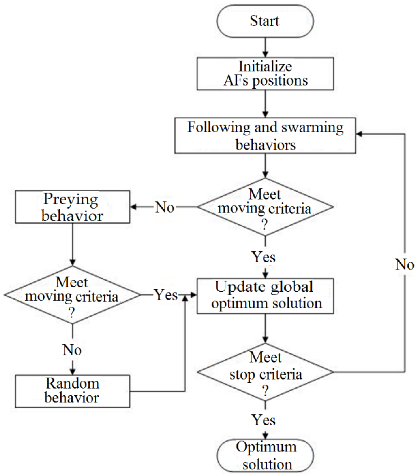
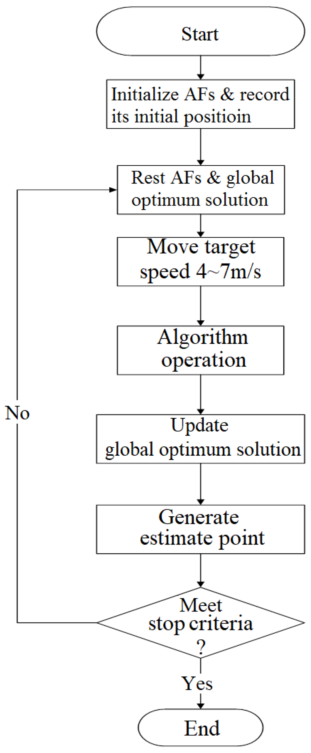
2.1.2. Flow Chart of AFSA

According to the previously described behavior, a movement strategy can be formulated. Each AF performs swarming and following behaviors, respectively. If it does not meet the movement requirements of the behavior, it carries out foraging behavior. If the movement requirements of the preying behavior are still not met, it carries out random behavior. After multiple moves to find the best solution in the whole domain, the AFSA process is shown in Figure 3.

2.1.3. Influence of Algorithm Parameters on System Convergence

The AFSA has five parameters, which are visual range Visual, step size Step, number of individuals M, number of tries Try_Number, and crowding factor δ [15,16,17,18,19,20,21,22,23]. The impact of each parameter on system convergence is summarized as follows:
Visual: When the Visual is small because each individual can see a relatively small number of other individuals in the algorithm at the same time, the ability of the individual to carry out swarming and following behaviors decreases, but the chance of the individual to search the adjacent area will also increase. The chances of individuals performing preying behaviors and random behaviors will also increase at this time. On the contrary, when the Visual is larger, the chances of individuals executing following behaviors and swarming behaviors will increase, while preying and random behaviors will decrease. Overall, the larger the Visual, the easier it is for the individual to find the global optimum solution, but it may also cause oscillations around the global optimum solution.
Step: The step size affects the accuracy and speed of the convergence of the algorithm. If a larger step size is selected, it can help the individual to converge to the extreme value quickly, but it may cause the individual to oscillate back and forth around the global optimum solution in the later stage of convergence, thus affecting the accuracy of convergence. If you choose a smaller step size, the convergence speed will be slower, but its accuracy is relatively better.
M: The larger the number of individuals is, the more information the individuals can exchange, the higher the accuracy of convergence, and the stronger the ability to jump out of the local optimum solution, but the greater the amount of calculation for each iteration of the algorithm. Therefore, in practical applications, on the premise of satisfying stable convergence, the number of algorithm individuals should be reduced as much as possible.
Try_Number: If the number of tries increases, the ability of the individual to perform preying behavior will increase, and the probability of the individual random moving will decrease. However, for problems with prominent local optimal solutions, if there are too many tries, it is easy for the individual to fall into the vicinity of the local optimum solution, thus missing the global optimum solution. Therefore, for general problems, the number of tries can be appropriately increased to speed up the convergence speed. For the problem with prominent local optimal solutions, the number of tries can be reduced to increase the probability of random movement of the individual to avoid falling into the local optimum solution.
δ: The crowd factor affects the results of the individual following and swarming behaviors. By combining the crowd factor with the field of view, it is possible to limit the swarming size of the individuals and further decide whether to perform the following and flocking behaviors. In the follow-up simulation experiments, we will ignore the crowding factor. In other words, as long as the AF Xi explores the state within the field of vision during flocking behavior or following behavior, as long as it is greater than the fitness value of Xi’s current position, it will move towards this state position regardless of overcrowding around the state.

2.2. RSSI Model

The RSSI channel model is also known as the Propagation Path Loss Model [24,25,26,27,28]. Under the free space propagation model, the signal intensity received by the receiver is inversely proportional to the square of the distance. When the distance between the transmitter and the receiver is d, the average power Pr(d) received by the receiver is as follows:
P r d = P t G t G r λ 2 4 π 2 d 2 L = P t G t G r λ 2 4 π 2 d 0 2 L · d 0 d 2 = P r d 0 · d 0 d 2
where Pt is the transmission power, Gt is the antenna gain at the transmitter, Gr is the antenna gain at the receiver, L is the system loss coefficient and represents the hardware signal loss in the communication system, λ is the wavelength, and d0 is the reference distance. In this study, the antenna gain of the transmitter and the receiver is set as one, which means that the system has no signal loss.
In general, the average loss P L ¯ ( d ) caused by the path is proportional to the nth power of the distance. In other words, at any distance between the transmitter and the receiver, the average loss at the receiver is as follows:
P L ¯ ( d ) = P L ¯ d 0 + 10 n × log d d 0
where n is the path loss index, which represents the path loss rate. In the natural environment, the interference received by the signal changes with the environment. Therefore, in the simulation analysis, we can only describe this phenomenon with logarithmic normal distribution, so the average power of the path can be expressed as
P L d = P L ¯ d + X σ = P L ¯ d 0 + 10 n · log d d 0 + X σ
and the received power can be expressed as
P r d = P t P L d
where P L ¯ ( d ) is the average path loss at the same distance between the transmitter and the receiver, Xσ is a zero-mean Gaussian random variable with a mean value of zero, and the standard deviation σ is 1 to 10 dBm. At the same distance between the transmitter and the receiver, the more complex the environment and terrain, the greater the fluctuation of the path loss means the larger the standard deviation. The reference distance is 0.5 m in subsequent simulation experiments.

3. System Model

This section will give a complete and detailed description of the AFSA-based wireless sensor network’s target positioning and tracking methods. The RSSI channel model is used to estimate the distance between the target point and the individual in the algorithm. Relying on the AFSA to simulate the creature preying characteristics, the highest point of the individual moving to find the food source (RSSI value) is regarded as the estimated point. In addition, this thesis also discusses the impact of sensor arrangement and quantity on the system.

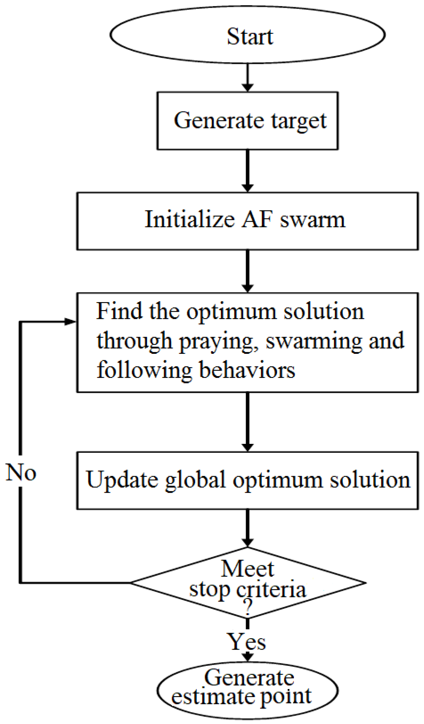
3.1. Target Positioning Method

The AFs (mobile sensors) were arranged on a square plane with an area of 100 m × 100 m. After each AF performs the algorithm behavior, the point with the highest food concentration (RSSI value) is obtained through communication with each AF as the global best solution. After a while, if the current global best solution meets the stop search condition, the corresponding position of the current global best solution is the estimated point, as shown in Figure 4.
In Figure 4, N target points are generated randomly. The optimum solution of the current time is obtained through the algorithm’s behaviors and compared with the global optimum solution. The bulletin board is a recording matrix with a size of 1 ×  Tmax, and Tmax is the maximum iteration value. This matrix records the best solution found in each iteration. After multiple iterations, if the stop criteria are met, the last value of the bulletin board is the estimated point.

3.1.1. Adaptive Step Size and Visual Range

Because the step size and field of view of AFSA will affect the performance of the system to find the optimal solution, the method of adaptive step size is proposed in [22] to improve the system performance. Therefore, this paper adds an adaptive step size and field of view method as shown in Equation (9) to the target positioning method and adopts a nonlinear dynamic adjustment of step size and field of view to meet the search requirements at various stages.
V i s a u l = V i s u a l × α + V i s u a l min S t e p = S t e p × α + S t e p min α = e 30 × t T max ζ
Here, ζ is the convergence factor and is an integer greater than one, which determines the convergence time of the curve. The larger the value, the later the convergence of the field of vision and step length; Visual is the field of vision; Step indicates the step size. In general, the initial value of Visual is networkSize/5 (networkSize is the maximum search range). The Step is Visual/8 [22]; Visualmin is the minimum value of the visual field; Stepmin is the minimum step size; t is the number of current iterations; Tmax is the maximum number of iterations. This method maintains the maximum value in the initial iteration, enabling the fish swarm to search the entire space approximately, improving the global search ability and convergence speed of the system. In the later iteration, the system changes to local search, keeping the visual field and step size at a low value, so that the region near the optimal solution can be searched for fine.

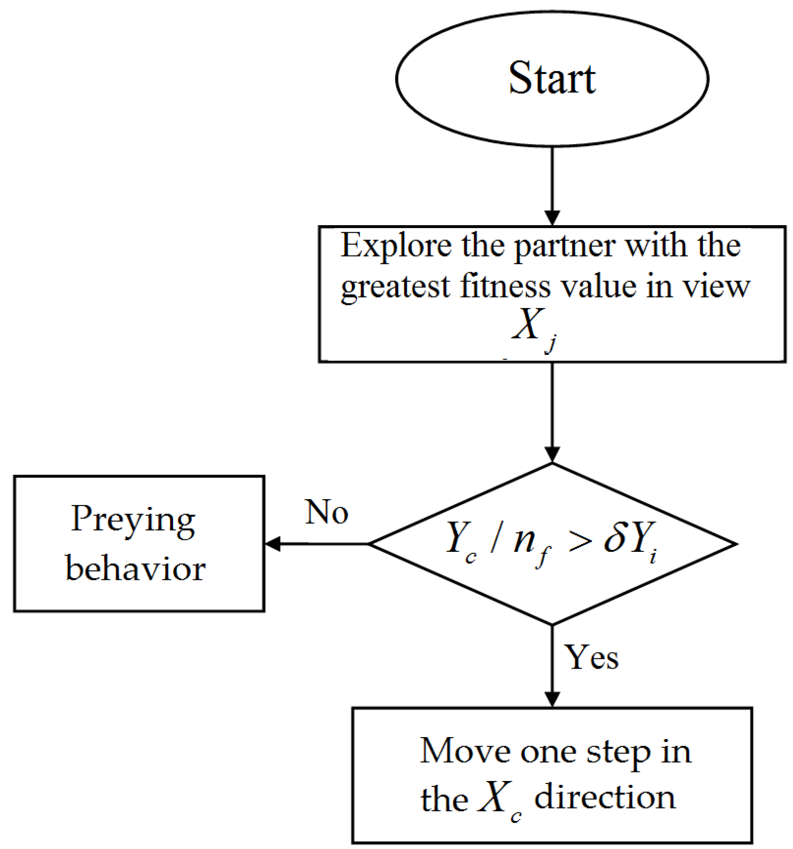
3.1.2. Hybrid Adaptive Vision of Prey

In this paper, based on the composite adaptive artificial fish swarm algorithm (AAFSA4) in [29], Hybrid Adaptive Vision of Prey (HAVP) is proposed to add a third fixed visual field, so that the method can better meet the needs of the positioning system.
In AAFSA4, the forward mode to the direction with a large fitness value is shown in Equation (10). The forward mode will slow down the search speed. Therefore, this paper takes AAFSA4 as the basis and changes the AF movement mode of the algorithm into a jumping mechanism, that is, when the AF searches for a better position Xj by the AAFSA4 method, the AF moves directly to this position, as shown in Equation (11). On the other hand, the three fields of vision can be searched with again to judge whether the forward condition is met. A search can be performed repeatedly until Try_number of times. If the forward condition is not met, one step of movement can be made randomly. In addition, this paper adds a third visual field, Visual3, which is the visual field of the fish swarm in the basic AFSA, and its value is a fixed value. The simultaneous random search of the three horizons can improve the efficiency of the system, but inevitably the complexity of the system will also be increased.
X n e x t = X + X V X X V X × S t e p × R a n d ( )
X n e x t = X j

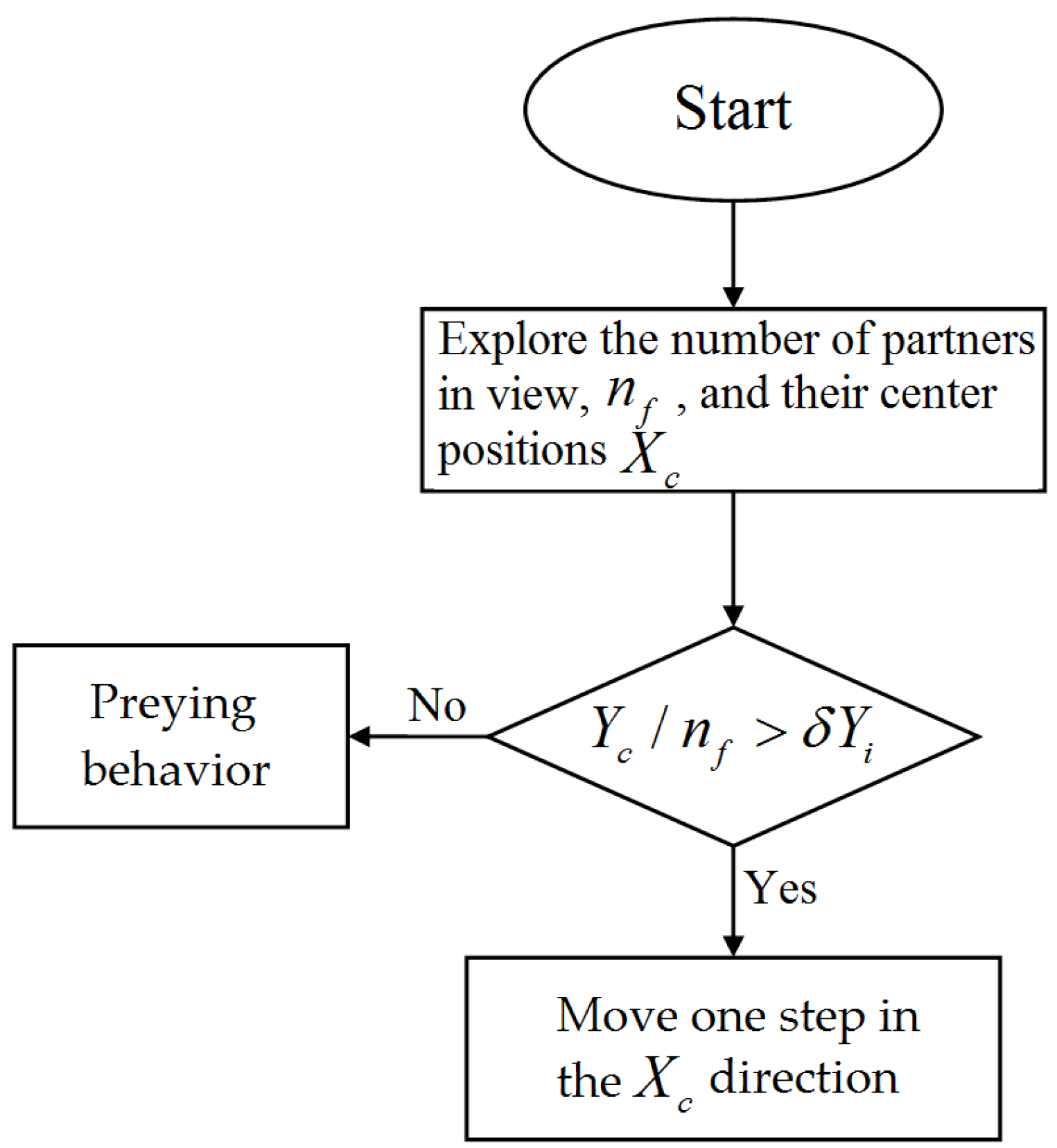
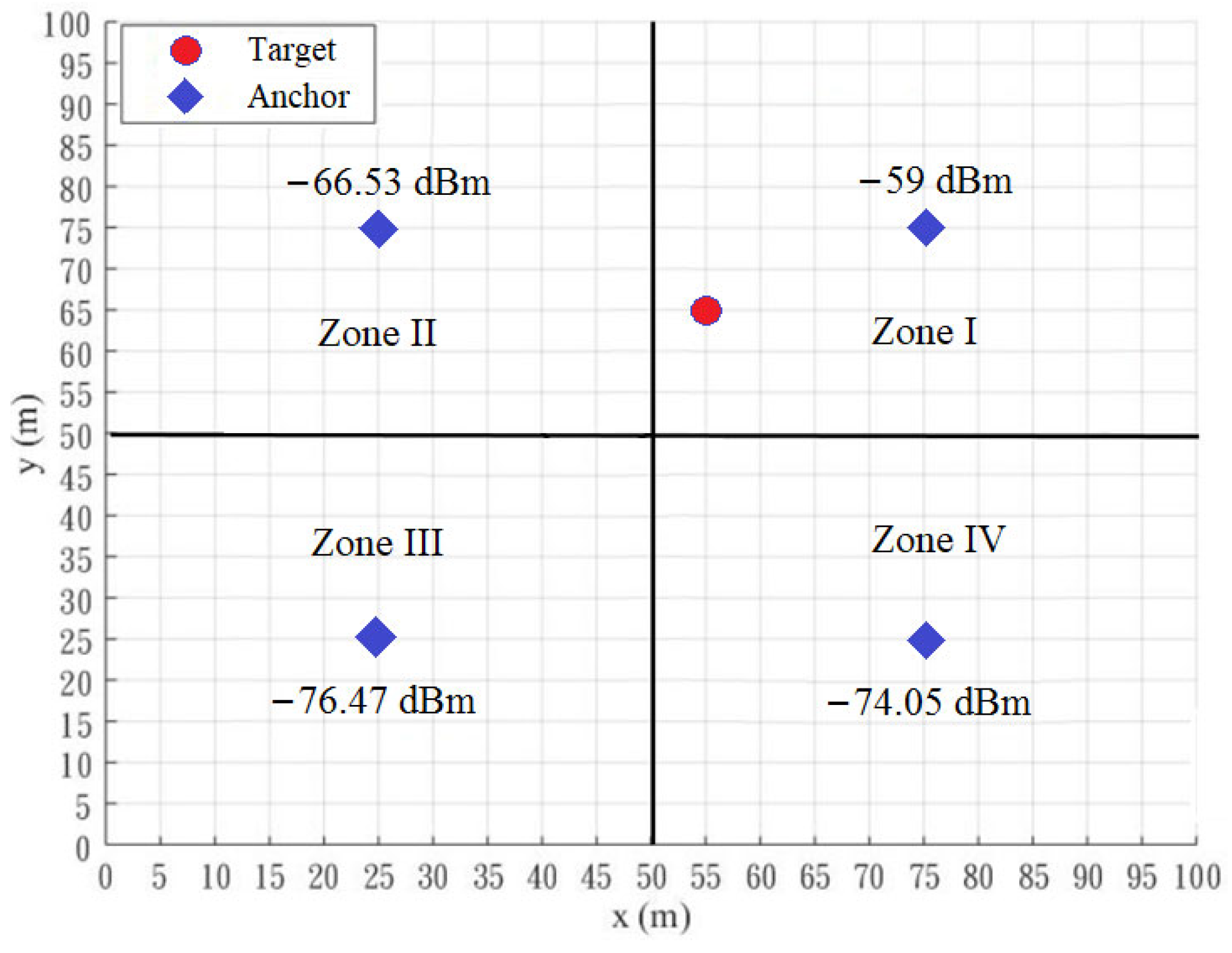
3.1.3. Region Segmentation Method [30]

The region segmentation method (RSM) involves dividing a 100 m × 100 m square wireless sensor network into four equal zones and positioning an anchor node in the center of each zone. The mobile sensor is equally divided into four segments and placed in each region. The anchor nodes of these four regions receive signal strength from the target point, and it is used to determine the approximate location of the target point. The boundaries [XL, XU, YL, YU] are defined, where XL represents the lower limit of the x axis, XU represents the upper limit of the x axis, YL represents the lower limit of the y axis, and YU represents the upper limit of the y axis. These boundaries restrict the movement of the individual particles to a specific range, and the algorithm uses this information to determine which region of the mobile sensor to focus on. Figure 5 is an illustration of RSM region judgment.

3.2. Target Tracking Method

Figure 6 is the AFSA target tracking flowchart [30]. The mobile sensors are deployed in a 100 m × 100 m square wireless sensor network. The AFs will gather in the highest fitness value region through Equation (12) as the estimated point. To avoid the algorithm dropping in a local solution, the global best will be reset to the initial value GlobalBest_Y = −100 in each iteration of finding the best one, so the algorithm can start another search.
Y i > G l o b a l B e s t _ Y G l o b l a B e s t _ Y = Y i

3.2.1. Tracks Definition

In this paper, two moving tracks, a snake track and a random track of target points, are designed in the target tracking method, as shown in Figure 7a,b. The moving speed is 4~7 m/s, so the students in the algorithm need to find the location of the target point within a limited number of moves. Therefore, the parameter setting of the algorithm is slightly different from the parameters of the algorithm in the target positioning method, such as step size and visual field. How to adjust the parameters in the algorithm so that the AFs can quickly find the target point is one of the problems discussed in this paper.

3.2.2. AF Movement Restriction in the Algorithm

Due to the moving characteristics of the target in the target tracking system, the target’s moving speed is 4~7 m/s. In other words, the AF needs to move as much as possible within one second and reach the set threshold value alpha, which affects the system’s success rate. If the signal strength received by the AF is greater than or equal to alpha, it is considered that the AF has found the target position and ended this search. The information, such as the current estimated point position and fitness value, is recorded in the record matrix for subsequent success rate calculation. On the other hand, the AF can perform the algorithm behavior within one second. If the fitness value of any AF does not reach alpha within one second, the AF with the highest fitness value among all AFs in the algorithm is selected as the estimated point. Figure 8 is the flow chart of the movement restriction of AFs in the algorithm. Equation (13) is the definition of success rate.
S = f i n d ( R e c o r d > a l p h a ) S u c c e s s R a t e = S T o t a l × 100 %
Here, S is the number of all estimated points reaching alpha. Record is the recording matrix, recording the fitness values of all estimated points. Total is the number of all estimated points.

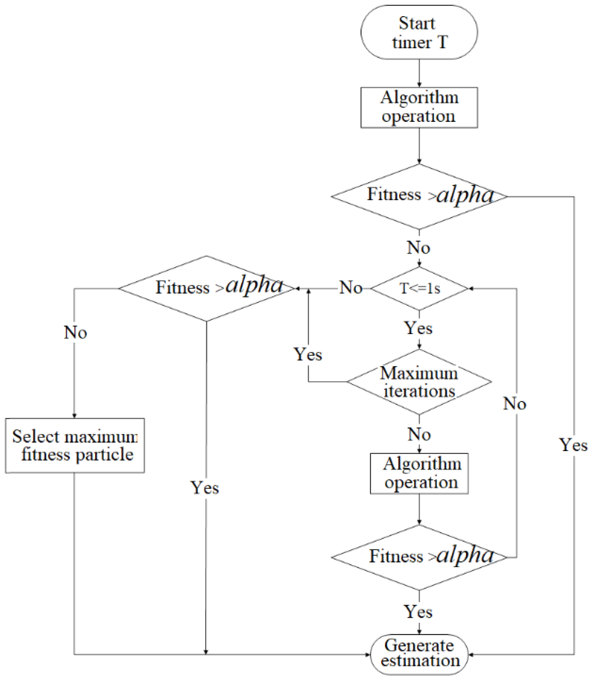
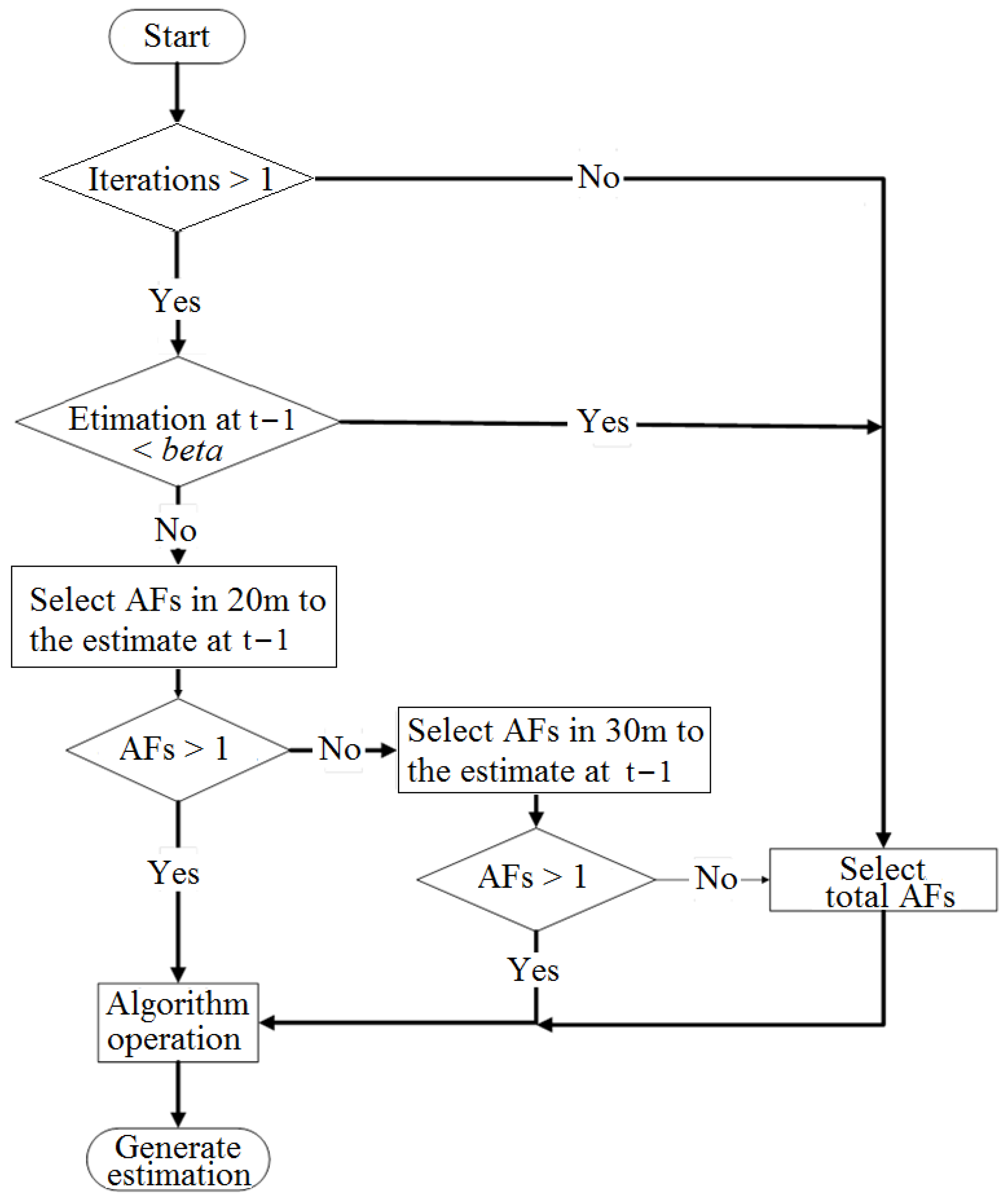
3.2.3. Dynamic AF Selection Method

For the AFSA target tracking system, a Dynamic AF Selection (DAFS) method is proposed in this paper to reduce the number of AFs used in the algorithm and reduce the search area to improve the efficiency of the target tracking system. This study assumes the target’s moving speed is 4~7 m/s, and the distance between the current and the previous target positions is very close. The DAFS method selects the AFs within 20 m from the last estimate point and starts a new algorithm iteration. If there is no AF in the range of 20 m, the AFs within 30 m are selected. Otherwise, all AFs will be considered in the algorithm. In addition, if the fitness value of the estimated point is less than the correction factor beta, all the AFs will be used in the algorithm to prevent error propagation. The DAFS method can reduce the search area and the number of AFs used in the algorithm to improve the efficiency of the target tracking system. Figure 9 shows the procedure of the DAFS method [30].

4. Simulation Results

4.1. Simulation Environment

In this study, the hardware and software used for simulations are listed in Table 1 [30]. The wireless sensor network is a two-dimensional area of 100 m × 100 m. The RSSI values will be calculated by substituting the position of each AF and the target point into the target function. The closer the location is to the target, the higher its RSSI value. In the simulation, each AF assumes to know the positions of other AFs. The AFs will move towards the area with the highest fitness value and eventually converge around the global optimum solution after many iterations by the algorithm. Then, the AF with the highest fitness value is selected as the estimated location.
In this paper, the AFSA was used with different numbers of AF for target positioning and tracking to investigate the impact of the number of AFs on the system. Additionally, the placement of the initial positions of the AFs was random deployment and the numbers of AF used in AFSA are 100, 72, 52, 24, 12, respectively, to address different applications in real-world environments.
The RSSI channel model parameters of the simulation experiment are shown in Table 2 [30], and Table 3 shows the AFSA simulation parameters for target positioning and tracking.

4.2. Simulation on Target Positioning

In order to calculate the error between the estimated point and the target point obtained by AFSA target positioning, the average error is calculated through Equation (14):
e = 1 N i = 1 N X ^ i X ^ i
where N is the number of target points, X ^ i is the position of the ith estimated point, and X i is the position of the ith target.
In this study, the performance of the proposed methods, RSM and HAVP, along with the adaptive step and adaptive vision methods, will be analyzed in terms of positioning accuracy. Various analysis modes are shown in Table 4. P1 and P2 are the traditional AFSA methods, and P3 to P8 are the proposed methods in this paper.
Table 5 shows the simulation results of the average error in random deployment, and the average positioning time is shown in Table 6. The average time is the average time required to locate a target point in 100 iterations using the MATLAB software calculation algorithm.

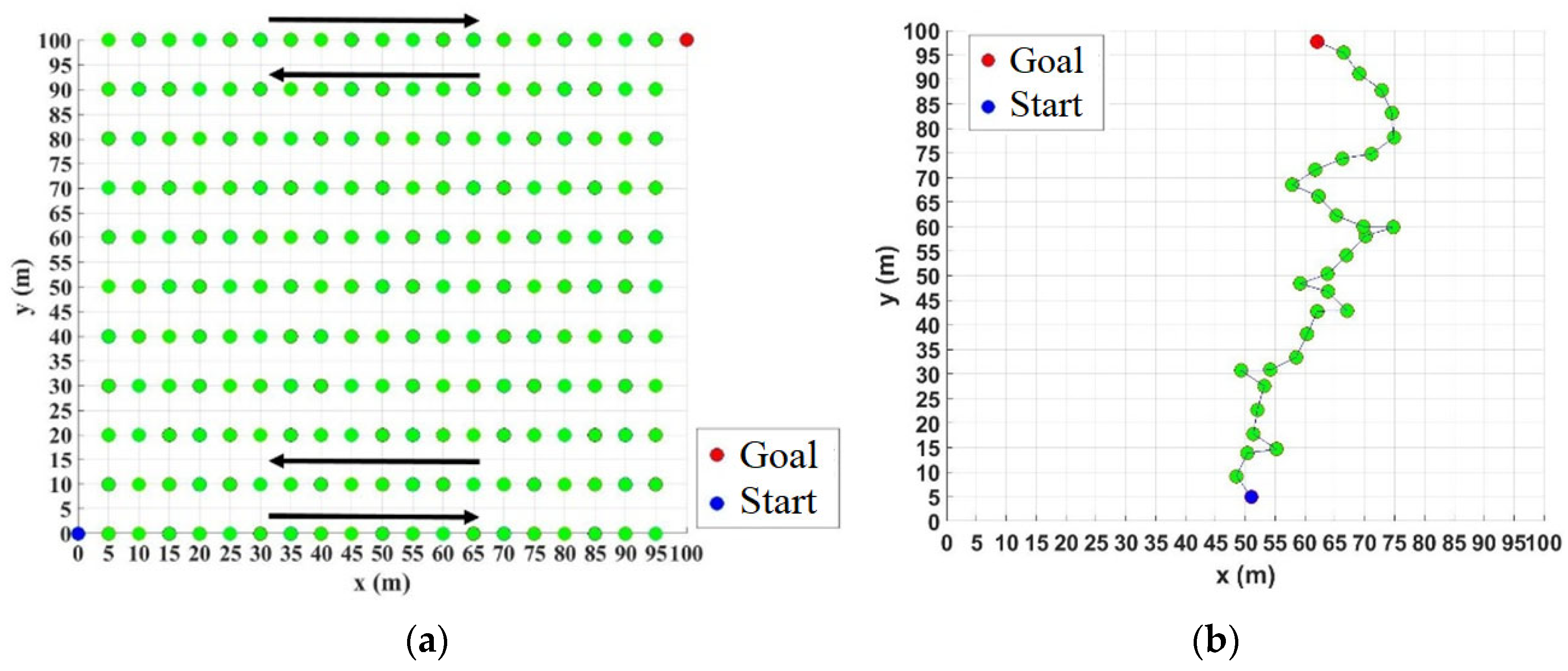
4.3. Simulation on Target Tracking

The methods proposed in this paper, such as RSM, HAVP, and DAFS, are added into the target tracking system, respectively. The analysis modes for the target tracking method are shown in Table 7 to analyze their influence on the system efficiency. In addition, in the simulation experiment, different numbers of AFs are placed in the sensor network for the simulation experiment of each analysis method, and the influence of the number of AFs in the algorithm on the system efficiency is discussed. K1 is a traditional method, and K2 to K8 are the proposed ones.
Table 8 shows the simulation results of the average tracking time, and the average tracking success rate is shown in Table 9. The average tracking time is the average time required to track a target point in 100 iterations using the MATLAB software calculation algorithm.

5. Discussion

5.1. Target Positioning

According to the simulation results in Table 5 and Table 6, some discussions for the target positioning system are as follows.
The average positioning error decreases as the number of AFs increases. The results in Table 10 were obtained based on the number of AFs. The average error is minimum at 100 AFs and becomes higher with the decrease in AFs. However, the average positioning time will increase with the increase in AFs because the more AFs there are, the longer the calculation time of the algorithm will be.
There is no significant difference between fixed step size and adaptive step size and visual field on positioning efficiency. According to Table 5 and Table 6, the values of all methods using fixed and adaptive step size are averaged, respectively, and the results are shown in Table 11. It shows that the simulation results of the fixed step size algorithm or the adaptive step size algorithm have little difference in the average positioning error and positioning time. The reason is that in the simulation environment of the wireless sensor network in this study, when there are a large number of AFs in the algorithm, whether it is a fixed or adaptive step size algorithm can satisfy the need to move AFs in the algorithm to the region of the global optimum solution within 100 iterations. On the contrary, when the number of AFs in the algorithm is fewer, such as reducing to 12, no matter the fixed step size or the adaptive step size, the AFs in the algorithm cannot move around the global optimum solution after 100 iterations.
RSM will increase the average error but greatly reduce the average positioning time. Table 12 shows the average error and positioning time of using and not using RSM. The average positioning error increases by about 26 cm, but the positioning time is shortened by 74.4%.
The HAVP method effectively improves the positioning error and positioning time. Table 13 shows the total average error and positioning time of using HAVP and not using HAVP. The average positioning error is reduced by about 96.1%, and the positioning time is shortened by 26.4%. If the analysis is carried out on whether to use RSM and HAVP, the results are shown in Table 14. It is obvious that using RSM will effectively improve the positioning time, but the positioning error will become worse. However, if the proposed HAVP is used, not only can the advantages of RSM to improve the positioning time be maintained, but the positioning error will not become worse.
For target positioning, the proposed AFSA algorithms, P7 and P8, combined with RSM and HAVP have better performance in both average error and average positioning time than the traditional AFSA methods, P1 and P2, in random deployment for target positioning. Especially in P8, the average positioning time is reduced by 81.9% compared with P2.

5.2. Target Tracking

From the simulation results in Table 8 and Table 9, the further discussions for target tracking can be depicted as follows.
RSM can use less time to achieve a better tracking success rate when there are many AFs, and the tracking performance of the modes without RSM is better when the number of AFs is fewer. Table 15 shows the total average positioning time and success rate of using RSM and not using RSM, which shows that the average positioning time of the analysis mode with RSM is less than that of the analysis mode without RSM. However, as the number of Afs used decreases, the difference between the average positioning time using RSM and those without RSM is smaller. The reason is that, after using RSM, the number of AFs used at the same time is less than that without RSM, so an AF in the AFSA can obtain less information from other AFs at the same time, so the AF needs to perform more algorithmic actions to reach the global optimal solution. Therefore, when the number of AFs is 12, the average positioning time using the RSM is longer than that without using the RSM.
When the number of AFs is large, using DAFS can shorten the positioning time and maintain a good tracking success rate. Analysis mode K1 without DAFS and K5 with DAFS were used to analyze the impact of DAFS on the performance of the target tracking system, as shown in Table 16. It can be found that the larger the number of AFS, the more data the algorithm needs to process, and the longer the target position estimation time is, and after using DAFS to track the AFSA target, it can be found that the greater the number of AFs used, the shorter the average positioning time. The reason is that when the DAFS method performs the algorithm by selecting the AF around the last estimated point, a larger number of AFs in the algorithm can ensure that there is an AF around the last estimated point and vice versa. The fewer the number of AFs, such as 12, the probability of an AF around the last estimated point is relatively small, so the use of all AFs for algorithm behavior increases, which in turn leads to the average positioning time when the number of AFs is 12. On the contrary, it is longer; in addition, when the number of AFs is greater than 52, DAFS can achieve a good tracking success rate at a faster speed, but when the number of AFs is less than 52, the DAFS method will make the system performance poor.
The average performance of the related modes using HAVP is shown in Table 17. It shows that using HAVP alone can improve the tracking success rate without increasing the positioning time. When using both DAFS and RMS for target tracking, the average positioning time of K8 is shorter by 42.47% than that of the traditional one, K1, and the average success rate remains the same as that of K1.

6. Conclusions

In this paper, AFSA is used to study indoor space target positioning and tracking. The simulation results show that the greater the number of AFs used in algorithm, the better the accuracy of target positioning but the longer the time of target positioning. The HAVP method is proposed to improve the positioning error and positioning time in this paper. The simulation results show that, when using HAVP, the total average positioning error is reduced by about 96.1%, and the positioning time is shortened by 26.4%. In addition, the DAFS method is proposed in the target tracking system to further reduce the number of AFs used in the target tracking system. The simulation results show that when the number of AFs is large, using DAFS can shorten the positioning time and maintain a good tracking success rate. Moreover, HAVP can improve the tracking success rate without increasing the positioning time. If DAFS and RMS are used at the same time, the positioning time can be greatly shortened by 42.47%, and the original success rate of the conventional method can be maintained.

Author Contributions

Conceptualization, C.-H.C. and Y.-F.H.; investigation, C.-H.C., C.-C.L. and Y.-F.H.; methodology, S.-H.L. and Y.-F.H.; software, C.-H.C. and C.-C.L.; supervision, C.-H.C. and Y.-F.H.; writing—original draft, C.-H.C., S.-H.L., C.-C.L. and Y.-F.H.; writing—review and editing, S.-H.L., C.-H.C. and Y.-F.H. All authors have read and agreed to the published version of the manuscript.

Funding

This research was funded by the Ministry of Science and Technology (MOST), R.O.C. grant numbers MOST 111-2221-E-324-018 and MOST-111-2637-E-150-001.

Data Availability Statement

Not applicable.

Conflicts of Interest

The authors declare no conflict of interest.

References

  1. Rajaravivarma, V.; Yang, Y.; Yang, T. An overview of Wireless Sensor Network and applications. In Proceedings of the 35th Southeastern Symposium on System Theory, Morgantown, WV, USA, 16–18 March 2003; pp. 432–436. [Google Scholar] [CrossRef]
  2. Corke, P.; Wark, T.; Jurdak, R.; Hu, W.; Valencia, P.; Moore, D. Environmental Wireless Sensor Networks. IEEE 2010, 98, 1903–1917. [Google Scholar] [CrossRef]
  3. Suo, H.; Wan, J.; Huang, L.; Zou, C. Issues and Challenges of Wireless Sensor Networks Localization in Emerging Applications. In Proceedings of the 2012 International Conference on Computer Science and Electronics Engineering, Hangzhou, China, 23–25 March 2012; pp. 447–451. [Google Scholar] [CrossRef]
  4. Xu, E.-Y.; Ding, Z.; Dasgupta, S. Target Tracking and Mobile Sensor Navigation in Wireless Sensor Networks. IEEE Trans. Mob. Comput. 2011, 12, 177–186. [Google Scholar] [CrossRef]
  5. Mesmoudil, A.; Fehaml, M.; Labraouil, N. Wireless Sensor Networks Localization Algorithms: A Comprehensive Survey. Int. J. Comput. Netw. Commun. 2013, 5, 1–20. [Google Scholar] [CrossRef]
  6. Cheng, L.; Wu, C.; Zhang, Y.; Wu, H.; Li, M.; Maple, C. A Survey of Localization in Wireless Sensor Network. Int. J. Distrib. Sens. Netw. 2012, 8, 12. [Google Scholar] [CrossRef]
  7. La, H.-M.; Nguyen, T.-H.; Hguyen, C.-H.; Nguyen, H.N. Optimal Flocking Control for a Mobile Sensor Network Based a Moving Target Tracking. In Proceedings of the IEEE International Conference on System, Man, and Cybernetics, San Antonio, TX, USA, 11–14 October 2009; pp. 4801–4806. [Google Scholar] [CrossRef]
  8. Laaraiedh, M.; Yu, L.; Avrillon, S.; Uguen, B. Comparison of Hybrid Localization Schemes using RSSI, TOA, and TDOA. In Proceedings of the IEEE Wireless Conference 2011-Substainalbe Wireless Technologies (European Wireless) 11th Europeanm, Vanna, Austria, 27–29 April 2011; pp. 1–5. [Google Scholar]
  9. Cheng, L.; Wu, C.-D.; Zhang, Y.-Z. Indoor Robot Localization Based on Wireless Sensor Networks. IEEE Trans. Comput. Electron. 2011, 57, 1099–1104. [Google Scholar] [CrossRef]
  10. Chugunov, A.; Petukhov, N.; Kulikov, R. ToA Positioning Algorithm for TDoA System Architecture. In Proceedings of the International Russian Automation Conference (RusAutoCon), Sochi, Russia, 6–12 September 2020; pp. 871–876. [Google Scholar] [CrossRef]
  11. Ahmed, S.; Abbasi, A.; Liu, H. A Novel Hybrid AoA and TDoA Solution for Transmitter Positioning. In Proceedings of the International Conference on Indoor Positioning and Indoor Navigation (IPIN), Barcelona, Spain, 4–7 October 2021; pp. 1–7. [Google Scholar] [CrossRef]
  12. Xu, C.-X.; Chen, J.-Y. Three-dimentional Sensor Node Localization based on AFSA-LSSVM. Int. J. Control. Autom. 2014, 7, 399–406. [Google Scholar] [CrossRef]
  13. Yang, X.; Zhang, W.; Song, Q. A Novel WSNs Localization Algorithm Based on Artificial Fish Swarm Algorithm. Int. J. Online Eng. 2016, 12, 64–68. [Google Scholar] [CrossRef]
  14. Wen, S.; Cai, X.; Guan, W.; Jiang, J.; Chen, B.; Huang, M. High-precision indoor three-dimensional positioning system based on visible light communication using modified artificial fish swarm algorithm. Opt. Eng. 2018, 57, 106102. [Google Scholar] [CrossRef]
  15. Li, X.-L.; Shao, Z.-J.; Qian, J.-X. An Optimizing Method Based on Autonomous Animats: Fish-swarm Algorithm. Chin. J. Circuits Syst. 2002, 22, 32–38. [Google Scholar] [CrossRef]
  16. Li, X.-L.; Qian, J.-X. Studies on Artificial Fish Swarm Optimization Algorithm based on Decomposition and Coordination Techniques. Chin. J. Syst. Eng. Theory Pract. 2003, 8, 1–6. [Google Scholar]
  17. Shan, X.-J.; Jiang, M.-Y.; Li, J.-P. The Routing Optimization Based on Improved Artificial Fish Swarm Algorithm. In Proceedings of the 6th World Congress on Intelligent Control and Automation, Dalian, China, 21–23 June 2006; pp. 3658–3662. [Google Scholar] [CrossRef]
  18. He, S.; Hamam, N.B.H.; Bouslimani, Y. Fuzzy Clustering with Improved Artificial Fish Swarm Algorithm. In Proceedings of the International Joint Conference on Computational Sciences and Optimization, Sanya, China, 24–26 April 2009; pp. 317–321. [Google Scholar] [CrossRef]
  19. Jiang, M.-Y.; Yuan, D.-F.; Cheng, Y.-M. Improved Artificial Fish Swarm Algorithm. In Proceedings of the Fifth International Conference on Natural Computation, Tianjin, China, 14–16 August 2009; pp. 281–285. [Google Scholar] [CrossRef]
  20. Cheng, Y.-M.; Jiang, M.-Y.; Yuan, D. Novel Clustering Algorithm Based on Improved Artificial Fish Swarm Algorithm. In Proceedings of the FSK 09. Sixth International Conference on Fuzzy System and Knowledge Discovery, Tianjin, China, 14–16 August 2009; pp. 141–145. [Google Scholar] [CrossRef]
  21. Fernandes, E.M.G.P.; Martins, T.F.M.C.; Rocha, A.M.A.C. Fish Swarm Algorithm for Bound Constrained Global Optimization. In Proceedings of the International Conference on Computational and Mathematical Methods in Science and Engineering, Asturias, Spain, 30 June–3 July 2009. [Google Scholar]
  22. Zhang, C.; Zhang, F.-M.; Li, F.; Wu, H.-S. Improved Artificial Fish Swarm Algorithm. In Proceedings of the 9th IEEE Conference on Industrial Electronics and Applications, Hangzhou, China, 9–11 June 2014; pp. 748–753. [Google Scholar] [CrossRef]
  23. Neshat, M.; Sepidnam, G.; Sargolzaei, M.; Toosi, A.N. Artificial fish swarm algorithm: A survey of the state-of-the-art, hybridization, combinatorial and indicative applications. Artif. Intell. Rev. 2014, 42, 965–997. [Google Scholar] [CrossRef]
  24. Fang, Z.; Zhao, Z.; Geng, D.; Xuan, Y.-D.; Du, L.-D.; Cui, X.-X. RSSI Variability Characterization and Calibration Method in Wireless Sensor Network. In Proceedings of the IEEE International Conference on Information and Automation, Harbin, China, 20–23 June 2010; pp. 1532–1537. [Google Scholar] [CrossRef]
  25. Xiong, J.-Q.; Qin, Q.; Zheng, K.-M. A Distant Measurement Wireless Localization Correction Algorithm Based on RSSI. In Proceedings of the Seventh International Symposium on Computation Intelligence and Design, Hangzhou, China, 13–14 December 2014; pp. 176–278. [Google Scholar] [CrossRef]
  26. Barsocchi, P.; Lenzi, S.; Chessa, S.; Giunta, G. A Novel Approach to Indoor RSSI Localization by Automatic Calibration of the Wireless Propagation Model. In Proceedings of the IEEE 69th Vehicular Technology Conference, Barcelona, Spain, 26–29 April 2009; pp. 1–5. [Google Scholar] [CrossRef]
  27. Mahmud, M.I.; Abdelgawad, A.; Yanambaka, V.P.; Yelamarthi, K. Packet Drop and RSSI Evaluation for LoRa: An Indoor Application Perspective. In Proceedings of the IEEE 7th World Forum on Internet of Things (WF-IoT), New Orleans, LA, USA, 14 June–31 July 2021; pp. 913–914. [Google Scholar] [CrossRef]
  28. Yao, L.; Peng, X.; Shi, D.; Liu, B. Design of Indoor Positioning System Based on RSSI Algorithm. In Proceedings of the International Conference on Management Science and Software Engineering (ICMSSE), Chengdu, China, 9–11 July 2021; pp. 145–148. [Google Scholar] [CrossRef]
  29. Hu, X.T.; Zhang, H.Q.; Li, Z.C.; Huang, Y.A.; Yin, Z.P. A Novel Self-Adaptation Hybrid Artificial Fish-Swarm Algorithm. In Proceedings of the 2013 IFAC, Hangzhou, China, 10–12 March 2013; Volume 46, pp. 583–588. [Google Scholar] [CrossRef]
  30. Lee, S.-H.; Cheng, C.-H.; Lin, C.-C.; Huang, Y.-F. PSO-Based Target Localization and Tracking in Wireless Sensor Networks. Electronics 2023, 12, 905. [Google Scholar] [CrossRef]
Figure 1. Flow chart of swarming behavior in AFSA.
Information 14 00246 g001
Figure 2. Flow chart of following behavior in AFSA.
Information 14 00246 g002
Figure 3. Flow chart of AFSA.
Information 14 00246 g003
Figure 4. Flow chart of AFSA target positioning method.
Information 14 00246 g004
Figure 5. Illustration of RSM region judgment.
Information 14 00246 g005
Figure 6. Flow chart of AFSA target tracking.
Information 14 00246 g006
Figure 7. Moving tracks of target points for the target tracking method: (a) snake track; (b) random track.
Information 14 00246 g007
Figure 8. Procedure of AF movement restriction in the algorithm.
Information 14 00246 g008
Figure 9. The procedure of DAFS method.
Information 14 00246 g009
Table 1. Simulation equipment.
NameSpecification
OSWindows 7 Enterprise 64 bits
CPUIntel(R) Core(TM) i5-4590 3.30 GHz
RAM8 GB
MATLAB EditionR2015a
Table 2. Parameters of RSSI channel model.
ParameterValue
Transmission Power Pt2 mW
Carrier Frequency f2.4 GHz
Path Loss Exponent n4.5
Reference Distance d00.5 m
Antenna Gains Gt, Gr1
Standard Deviation σ9 dBm
Table 3. AFSA parameters for target positioning and target tracking.
ParameterValue
Target PositioningTarget Tracking
Network size100 m × 100 m
Number of executions100
Number of iterations Tmax100
Number of sensors M100, 72, 52, 24, 12
Number of targets N101
Try number Try_Number100
Initial step StepVisual/8 2
Initial visual VisualnetworkSize/5 2
Minimum step Stepmin5 1,2
Minimum visual Visualmin50 1,2
Convergence factor S4 2
Threshold alpha*−6.5 dBm
Correction factor beta*−15 dBm
1 For fixed step and visual; 2 for adaptive step and visual; * not applicable.
Table 4. Analysis modes for target positioning method.
ModeCondition
Fixed StepAdaptive Step and VisionRSMHAVP
P1
P2
P3
P4
P5
P6
P7
P8
Table 5. Average error of random deployment in target positioning.
Number of AFP1P2P3P4P5P6P7P8
1000.8740.8922.5162.5620.0000.0000.0000.000
721.1171.1133.3593.3580.0000.0000.0000.000
541.6141.5004.3204.4180.0000.0000.0000.000
242.9532.9918.3708.6940.0000.0000.0000.000
125.5205.341251.316231.7050.1210.00011.16210.247
Average2.4162.36753.97650.1470.0240.0002.2322.049
Table 6. Average positioning time of random deployment in target positioning.
Number of AFP1P2P3P4P5P6P7P8
10012.98613.7903.4063.1919.18410.0182.3822.363
728.9169.6132.2032.5416.5467.6421.7491.650
546.6346.7501.6241.7874.7784.9961.3621.236
242.9743.0850.8600.7822.1082.2360.6760.732
121.3261.3520.1740.2061.0491.1760.3080.290
Average6.5676.9181.6531.7014.7335.2141.2951.254
Table 7. Analysis modes for target tracking method.
ModeRSMHAVPDAFS
K1
K2
K3
K4
K5
K6
K7
K8
Table 8. Average tracking time of random deployment in target tracking.
Number of AFK1K2K3K4K5K6K7K8
1000.0810.0580.0760.0400.0410.0320.0400.026
720.0650.0410.0670.0300.0380.0340.0410.028
540.0610.0430.0610.0330.0510.0480.0400.032
240.0440.0390.0460.0230.1090.0980.0420.038
120.0410.0640.0370.0580.1230.1090.0480.044
Average0.05840.0490.05740.03680.07240.06420.04220.0336
Table 9. Average tracking success rate of random deployment in target tracking.
Number of AFK1K2K3K4K5K6K7K8
10099%81%100%83%100%97%100%98%
7299%100%100%100%99%99%98%99%
54100%100%100%99%95%96%97%96%
2497%100%99%95%85%94%96%96%
1294%76%100%85%85%80%95%97%
Average97.8%91.4%99.8%92.4%92.8%93.2%97.2%97.2%
Table 10. Total average error and positioning time when the number of AFs is 100, 72, 54, 24, and 12.
Number of AFAverage Error (cm)Average Positioning Time (s)
1000.8497.272
721.1215.081
541.4673.638
242.8391.658
1266.0640.741
Table 11. Total average error and positioning time of the fixed and adaptive steps.
ParameterFixed StepAdaptive Step
Average error (cm)14.58914.347
Average positioning time (s)3.5873.587
Table 12. Total average error and positioning time of using and not using RSM.
ParameterNo RSMRSM
Average error (cm)1.18527.750
Average positioning time (s)5.8661.490
Table 13. Total average error and positioning time of using and not using HAVP.
Parameter No HAVPHAVP
Average error (cm)27.8611.074
Average positioning time (s)4.2373.120
Table 14. Average error and positioning time for methods using and not using RSM and/or HAVP.
ParameterNo RSM + HAVPRSMHAVPRSM + HAVP
Average error (cm)2.3653.360.012.14
Average positioning time (s)6.761.714.971.27
Table 15. Total average positioning time and success rate of methods using or not using RSM.
Number of AFAverage Positioning Time (s)Average Success Rate
No RSMRSMNo RSMRSM
1000.0600.03999.8%99.5%
720.0530.03399.0%99.5%
540.0530.03998.0%97.8%
240.0600.05094.3%96.3%
120.0620.06993.5%84.5%
Table 16. Average positioning time and success rate of modes K1 and K5.
Number of AFAverage Positioning Time (s)Average Success Rate
K1K5K1K5
1000.0810.04199%100%
720.0650.03899%99%
540.0610.051100%95%
240.0440.10997%85%
120.0410.12394%85%
Table 17. Average positioning time and success rate for K1, K3, K7, and K8.
ParameterK1K3K7K8
Average positioning time (s)0.05840.05740.04220.0336
Average success rate97.8%99.8%97.2%97.4%
Disclaimer/Publisher’s Note: The statements, opinions and data contained in all publications are solely those of the individual author(s) and contributor(s) and not of MDPI and/or the editor(s). MDPI and/or the editor(s) disclaim responsibility for any injury to people or property resulting from any ideas, methods, instructions or products referred to in the content.

