Article

Anomaly Detection Approach in Industrial Control Systems Based on Measurement Data

School of Artificial Intelligence and Data Science, Hebei University of Technology, Tianjin 300132, China
*
Author to whom correspondence should be addressed.
Information 2022, 13(10), 450; https://doi.org/10.3390/info13100450
Submission received: 24 August 2022 / Revised: 21 September 2022 / Accepted: 23 September 2022 / Published: 25 September 2022
(This article belongs to the Special Issue Advances in Computing, Communication & Security)

Abstract

:
Anomaly detection problems in industrial control systems (ICSs) are always tackled by a network traffic monitoring scheme. However, traffic-based anomaly detection systems may be deceived by anomalous behaviors that mimic normal system activities and fail to achieve effective anomaly detection. In this work, we propose a novel solution to this problem based on measurement data. The proposed method combines a one-dimensional convolutional neural network (1DCNN) and a bidirectional long short-term memory network (BiLSTM) and uses particle swarm optimization (PSO), which is called PSO-1DCNN-BiLSTM. It enables the system to detect any abnormal activity in the system, even if the attacker tries to conceal it in the system’s control layer. A supervised deep learning model was generated to classify normal and abnormal activities in an ICS to evaluate the method’s performance. This model was trained and validated against the open-source simulated power system dataset from Mississippi State University. In the proposed approach, we applied several deep-learning models to the dataset, which showed remarkable performance in detecting the dataset’s anomalies, especially stealthy attacks. The results show that PSO-1DCNN-BiLSTM performed better than other classifier algorithms in detecting anomalies based on measured data.

1. Introduction

ICSs are used to control physical processes in industry and critical infrastructure [1]. They are used in a wide variety of operations, such as industry, energy, transportation, and municipalities [2]. Hence, they are integral to the safety and security of a nation’s critical infrastructure. Due to their critical nature, attacks on ICSs [3] that propagate to physical processes can cause large monetary losses, incur environmental damage, and significantly impact the infrastructure of cities [4]. Well-known attacks such as the Stuxnet worm in 2010 [5], an attack on a steel plant in Germany by criminals in 2014 [6], a U.S. water treatment plant hacked by a Syrian hacktivist group in 2015 [7], and the hijacking of the U.S. fuel pipeline system in 2021 demonstrate the impact and consequences of ICS attacks [8].
Although industrial control system security and traditional information security have many similarities, and many security requirements are similar, they still have big differences [9]. Traditional information security is oriented to data management, while industrial control security is oriented to equipment control. In traditional information security, the confidentiality of data is given top priority, and the practicality of security policies is the first consideration in industrial control security systems [10]. Traditional information security equipment has a high update frequency, while industrial control security equipment has poor compatibility and a long system update cycle. Compared to traditional information security, the application protocol structures of ICSs are simple and do not support encryption. When an ICS accesses the network [11] for work, it is easy to attack from a server vulnerability, thus leading to abnormal control logic. Therefore, traditional information security field methods can not be directly applied to industrial control security issues.
In recent years, with the development of industrial informatization, the security of industrial control systems has become increasingly prominent, and the demand for security research in related fields is growing. In the face of the characteristics of industrial control systems themselves, it is of great significance to be able to effectively detect anomalies and stop the propagation of risks.

2. Related Works

Many researchers have started focusing on developing techniques and approaches for anomaly detection within ICS processes. Existing methods for detecting anomalies in industrial control systems can be divided into three categories:
(I)
An industrial control anomaly detection method based on protocol feature rules [12], which analyzes the protocol specification under normal conditions and establishes detection rules to detect anomalies that do not conform to the specification [13]. For example, Nasr et al. analyzed the alarm properties of SCADA to achieve anomaly detection in smart grids through statistical methods [14]. The disadvantage of this approach is that it is not sensitive enough to the sequence of attack events and internal relationships.
(II)
An industrial control anomaly detection method based on the system behavior state [15], which statistically analyzes the parameters of the industrial control system and establishes the normal behavior profile of the system for anomaly detection. Khalili et al. analyzed the information for a normal state from historical data and used the Apriori algorithm to implement anomaly detection [16]. Kwon et al. analyzed the communication behavior and protocol characteristics of smart substations and proposed a behavior-based anomaly detection method [17]. The disadvantage of this approach is that it cannot detect potential attack operations that exploit system vulnerabilities or masquerade as normal behavior.
(III)
Embedded machine learning-based industrial control anomaly detection method [18]. Machine learning methods are widely used in the fields of data mining and target detection [19]. Now that embedded machine learning methods are rapidly developing in industrial automation, researchers are trying to use their methods to mine communication data and build models for anomaly detection. Yap et al. [20] used tiny machine learning (TinyML) on an embedded system to identify data out of the expected range in the system in order to enable anomaly detection in industrial equipment. Narjes et al. [21] used a sparse autoencoder (SAE) network for anomaly detection of air conveyors in railroads and were able to effectively detect failures due to air leakage problems. Matteo et al. [22] designed machine learning algorithms executed on microprocessors, deployed on distributed sensors for the Internet of Things, capable of detecting anomalies in the status of bearings and proactively shutting down abnormal machines. This method may have disadvantages such as reduced efficiency in handling large-scale data, inability to solve the imbalance of sample distribution and easy to fall into local optimum, and its algorithm detection accuracy still has much room for improvement.
These methods can achieve anomaly detection with reasonable accuracy in the right application scenario, but they typically use network traffic for anomaly detection, which is inefficient in detecting internal corruption or natural system anomalies. In addition, network traffic usually has appropriate security measures in place, causing these methods to ignore anomalies caused by encryption or any other forged packets.
For the methodology presented in this paper, instead of monitoring the network traffic, we investigated suspicious activities in the system’s measurement data. ICSs deployed in microcontrollers have a limited role in monitoring network traffic, but they are capable of measuring a variety of parameters, and these measurements can be well-used in a variety of anomaly detection areas [23]. Because measurement data is a true reflection of the working state of an ICS, anomaly detection based on measurement data is more effective than monitoring network traffic in order to address these issues [24]. This fault-detection approach can find any deviation from normal performance caused by malicious activities, such as changing the sensors’ setpoints or injecting fake data measurements into the ICS network levels. It can be used for precise and quick detection of anomalous behaviors in time-series data from industrial infrastructure.

3. Methodology

In this paper, a model structure combining 1DCNN and BiLSTM was used as the basis, and PSO was implemented to optimize the hyperparameters of the model; the theory related to these methods is described below.

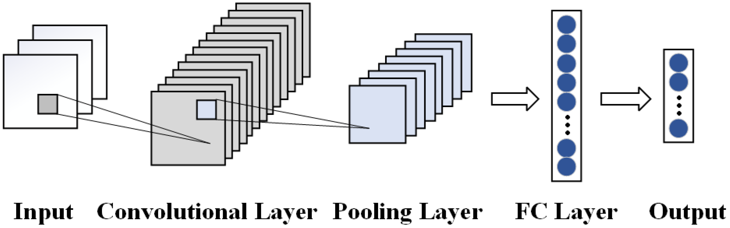
3.1. 1D Convolutional Neural Network

Convolutional neural networks (CNNs) are widely used to extract local characteristics for the normal and attack classifications. Given an input signal, a CNN with these filters can extract temporal locality from inputs and help learn temporal dependencies in multivariate time-series input data. Therefore, 1DCNN [25] can efficiently learn temporal and spatial dependencies within time-series sensor and actuator input data.
As shown in Figure 1, a CNN works through a composition of the convolutional layer, the activation function, the pooling layer, and the fully connected (FC) layer [26]. The activation function is used to add a nonlinear relationship to the result of the convolution operation. The pooling layer is used to extract important features from the output of the convolutional layer. During the pooling process, the output dimension of the convolutional layer is reduced but the learned important features are retained.
The formula for the 1DCNN is:
Z l + 1 = x = 1 f [ Z k l ( s 0 + x ) w k l + 1 ( x ) ] + b
where Z l is the input to the l + 1 layer convolution, Z l + 1 is the output, b is the bias, w k l + 1 is the weight, f is the convolution kernel size, and s 0 is the convolution step size.
The activation function used in this article is the RELU function; the formula for the RELU function is:
f ( x ) = max ( 0 , x )
The pooling layer used in this article is MaxPooling; the formula for MaxPooling is:
y i l + 1 ( j ) = max x i j ( k ) , k D j
where y i l + 1 is the i-th feature map of layer l + 1 after pooling, D j is the range where the pooling operation is performed, and x i j is the element in the pooling range.
The formula for the fully connected layer is:
Y = X A T + B
where X is the input matrix, A T is the transpose of the fully connected layer parameter matrix, and B is the deviation.

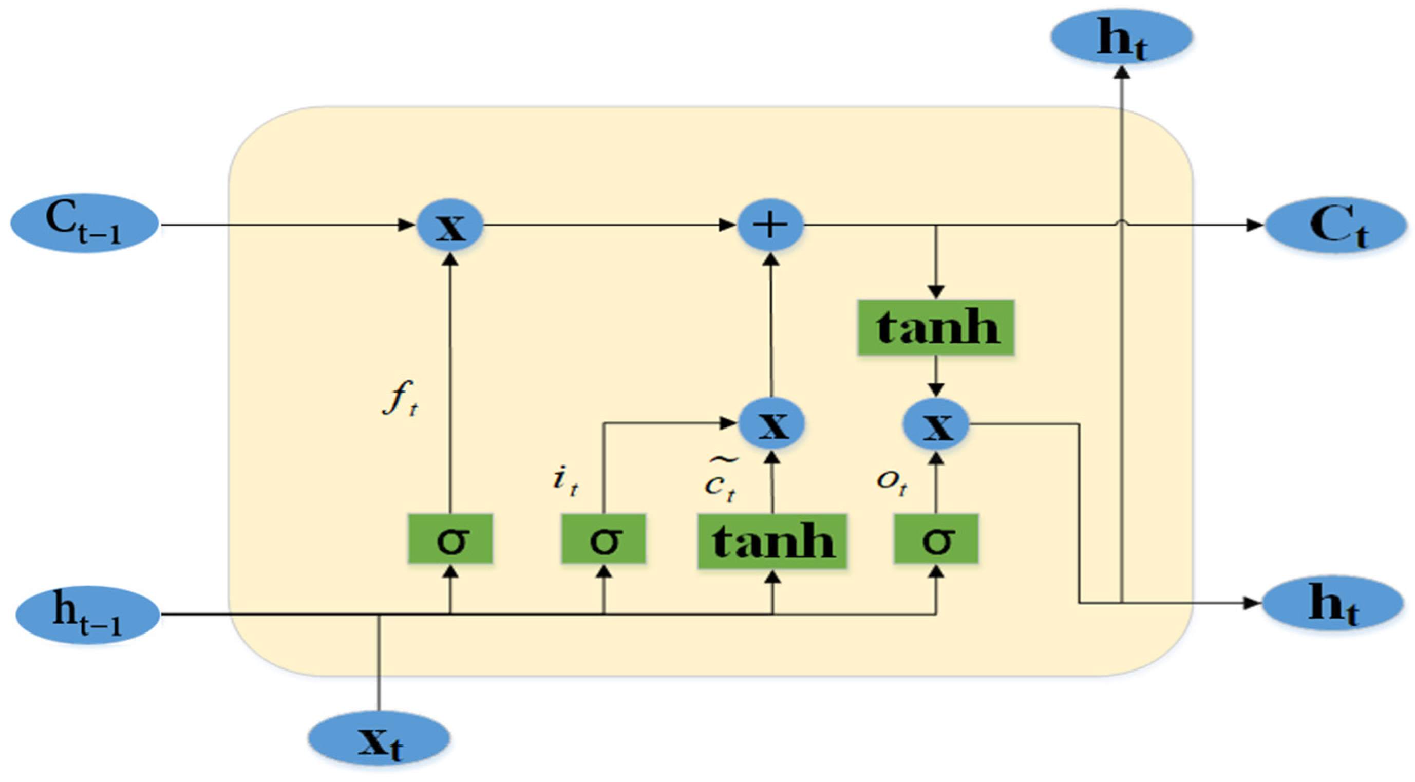
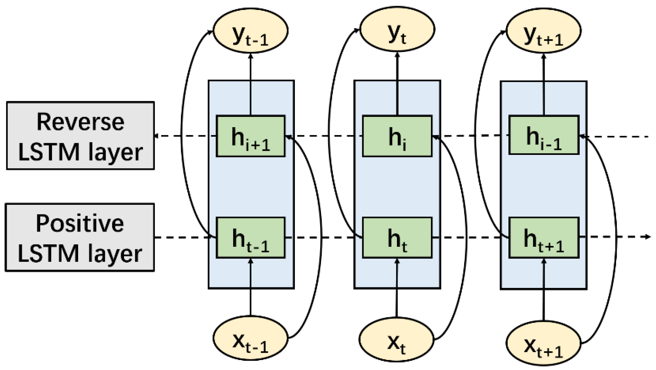
3.2. Bidirectional Long Short-Term Memory Network

A long short-term memory network (LSTM) [27], which is an extended form of an RNN [28], is used to detect temporal patterns in sensor/actuator time series data. An LSTM hidden state at the time step t is computed by:
I n p u t _ G a t e : i t = σ ( W i x t + U i h t 1 + b i )
F o r g e t _ G a t e : f t = σ ( W f x t + U f h t 1 + b f )
O u t p u t _ G a t e : o t = σ ( W o x t + U o h t 1 + b o )
C e l l _ I n p u t : c t ˜ = tanh ( W c x t + U c h t 1 + b c )
C e l l _ S t a t e : c t = i t c t ˜ + f t c t 1
C e l l _ O u t p u t : h t = o t tanh ( c t )
where σ and tanh are the element-wise sigmoid and hyperbolic tangent functions. h t 1 and c t 1 are the hidden state and memory cell of the previous time step. W i , W f , W o , W c , b i , b f , b o , b c are the training parameters.
In this context, LSTM defines the influence of the sensor/actuator input by using a sigmoid layer for each gate to be open or closed. As depicted in Equations (5)–(7), i t , f t , and o t are input, forget, and output gates. In Equation (8), c t ˜ , which is the recurrent unit, is calculated based on the input at the current time x t and the hidden state of the previous time step h t 1 . In (10), h t is the current hidden state of the LSTM at time t through tanh activation, and in (9) the memory cell, c t , is calculated. The memory cell identifies the contribution of the previous time step and the current input to calculate the hidden state h t . Figure 2 depicts this mechanism in detail.
BiLSTM is a bidirectional variant of LSTM that connects two hidden layers of opposite directions to the same output [29]. Compared with LSTM, the hidden layer of BiLSTM is split in two directions, forward (from past to future) and backward (from future to past). A BiLSTM hidden layer at the time step t is computed by:
h t = L S T M ( x t , h t 1 )
h i = L S T M ( x t , h i 1 )
H t = b t h t + b i h i + c t
where h t and h i are the two-way hidden layer states at the current moment, b t and b i are the two-way hidden layer output weights at the current moment, and c t is the bias parameter at the current moment.
Figure 3 illustrates the functional diagram of BiLSTM. One LSTM network processes the sequence from the left to the right (forward) and the other processes the sequence from the right to the left (backward). At each time step t , the forward pass calculates the hidden state h t by considering the previous hidden state h t 1 and the new input sequence x t . At the same time, the backward flow calculates the hidden state h i considering the future hidden state h i 1 and the current input x t . Afterward, the forward h t and the backward h i are concatenated to obtain the combined vector representation.

3.3. Particle Swarm Optimization

PSO is a global optimization algorithm that uses particles to discover a search space and converge on the global minimum. The algorithm spreads these particles over the search space and iteratively moves their location based on previous best locations and stochastic variables [30].
The first step of PSO is to initialize the particles around the search space. Each particle is then given a random velocity and the algorithm moves onto its cyclical phase. The particles move in accordance with their current velocity for one step. Then, the current function value of each particle is calculated at its new location. If a particle’s current value is less than its previous best personal value, its personal best is updated to this value. If any of the particles have a value lower than the previous global best value, the global best is updated to this value. Following this, the velocities of each particle are updated. The equation for the updated velocity and the updated position are:
v i ( t + 1 ) = w v i ( t ) + c 1 r 1 ( p i ( t ) x i ( t ) ) + c 2 r 2 ( g ( t ) x i ( t ) )
x i ( t + 1 ) = x i ( t ) + v i ( t + 1 )
where v i and x i are the velocity and position of the particle, c 1 and c 2 are acceleration factors, w is the weight parameter, r 1 and r 2 are random variables, and p i and g are the historical optimal position of the particle and the global historical optimal position, respectively.

3.4. Other Methods

To convert an array into a one-dimensional array to facilitate computation, the f l a t t e n method is used.
In this work, a specific type of convolution layer was used, known as a multi-branch shallow convolution layer. To operate the input tensor sequences in series, the c a t method in the PyTorch framework was used. The formula for the cat method is:
o u t = c a t ( i n p u t , dim )
where i n p u t is the tensor sequence to be connected and dim is the dimension selected for expansion, ranging from 0 to the length of each dimension sequence in i n p u t .
To portray the distance between the actual output and the expected output, the C r o s s E n t r o p y L o s s method was used. The formula is:
H ( p , q ) = x p ( x ) log q ( x )
where p is used to denote the desired output, q denotes the actual output, q ( x ) maps the output to a range from 0 to 1 and is used to denote the probability of the output, p ( x ) is the label, which is the desired output, and finally, the cross-entropy is obtained by removing the negative sign and then finding the mean value.
In this work, the S G D method was used as an optimizer to implement gradient descent in training; the formula for calculating the variation of weights and gradients in S G D is:
θ = θ α ( θ )
L ( θ ) = L ( θ ) + ( θ w e i g h t )
where θ is the learnable parameter, α is the learning rate decay, L ( θ ) is the gradient, and w e i g h t is the weight decay.

4. Proposed Model

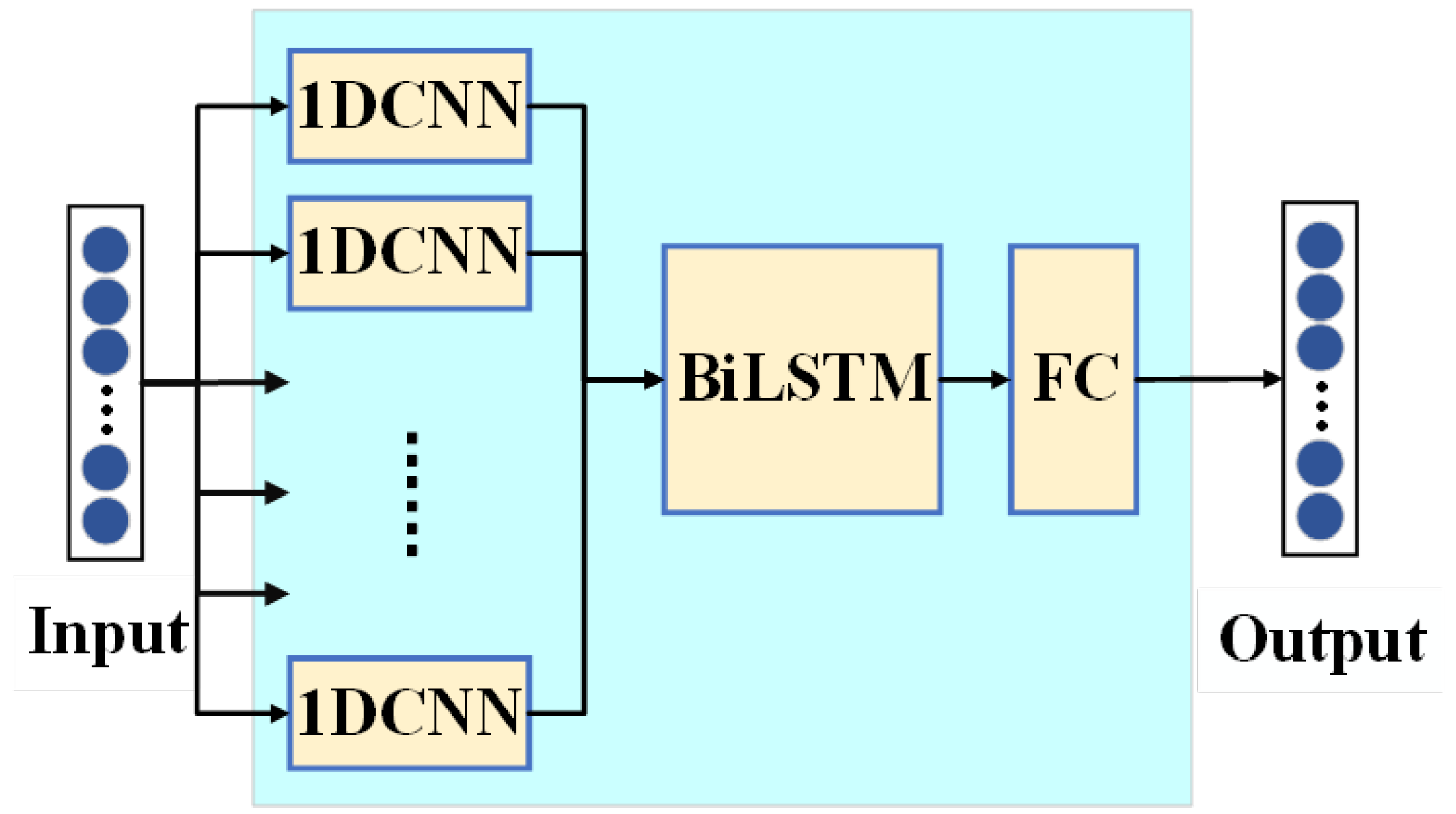
4.1. Algorithm Overview

For the model structure of deep learning methods, the change of hyperparameters will affect the model more significantly, and the reasonable tuning of parameters is also quite an important process for model training. The PSO method has a good effect on the merit treatment of nonlinear problems, so the hyperparameters of the algorithm model were selected optimally using the PSO method before entering the training process formally.

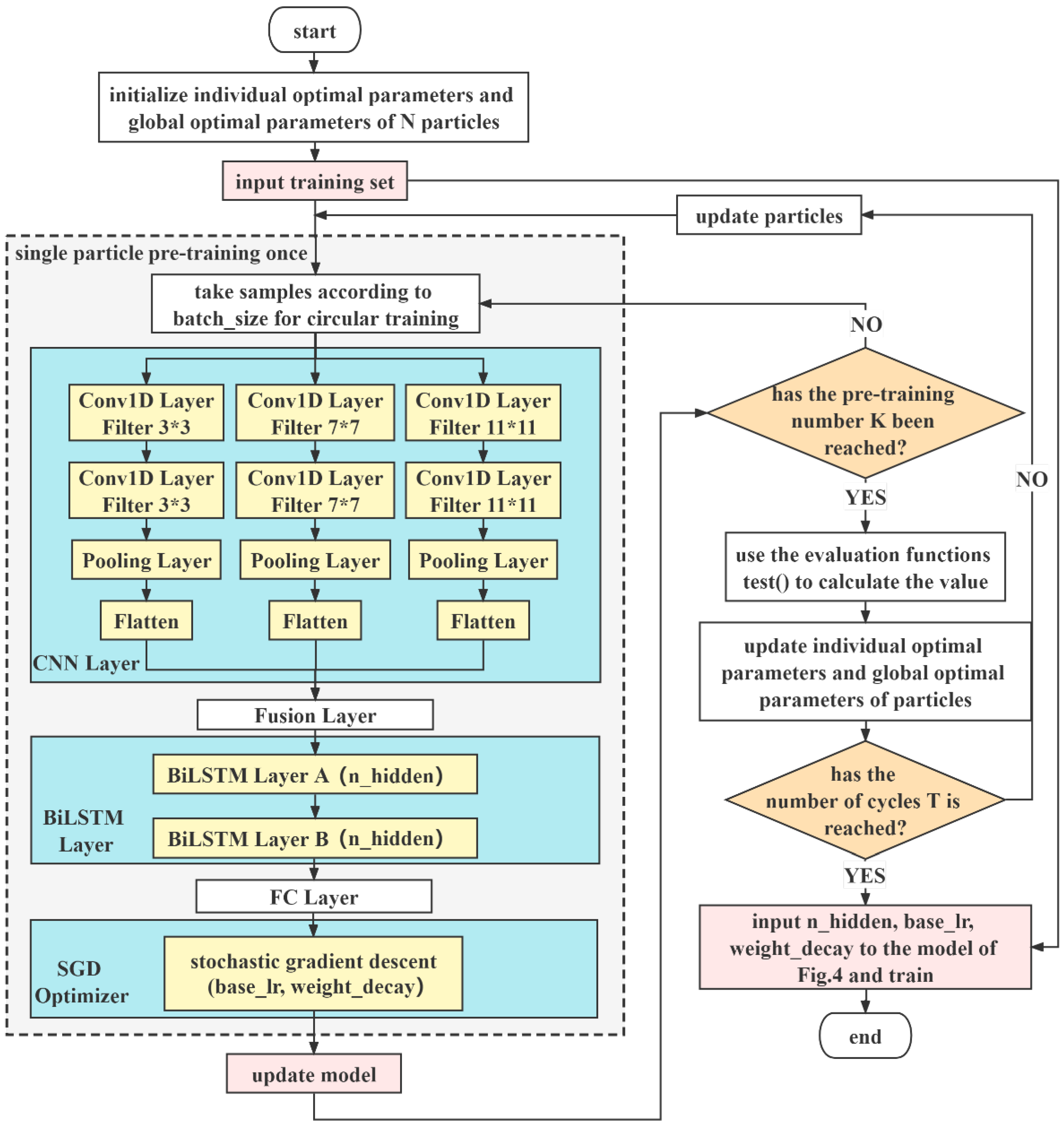
4.2. Model Structure and Algorithm Flow

In this work, we propose a 1DCNN-BiLSTM model, as shown in Figure 4. The model consists of three major components: the 1DCNN layer, the BiLSTM layer, and the FC layer. The 1DCNN layer can have multiple branches, which are used to capture different temporal local dependencies by using different sizes of convolutional kernels. These branches are similar, having the same input and different convolutional kernel sizes. The outputs of the 1DCNN layer were transformed into a one-dimensional array by using the Flatten layer, which was fed to the BiLSTM layer as input data through splicing. The FC layer acts as the interface between the BiLSTM layer and the BatchNorm1d method. Lastly, the SGD neural network optimizer acted as the method for performing gradient descent during the training process.
The realization of Algorithm 1 that uses the PSO method optimally selects the hyperparameters of the algorithm model to accelerate the training process. The hyperparameters contain three dimensions, which consist of the number of hidden layers (n_hidden), the learning rate decay (base_lr), and the weight decay (weight_decay). The schematic diagram in Figure 5 helps visualize how PSO was applied in Algorithm 1.
The overall framework for optimization using the PSO method is shown in Figure 5, and the algorithm flow was as follows:
(1) Preprocessing of the raw data. The range of values between each dimension of the raw data is so large that direct use would result in a gradient explosion during training. After removing noise data from the original data, the data are normalized by dividing each dimension by the maximum absolute value of that dimension, so that each dimension is scaled to a floating-point number between minus one and one.
(2) Initialize the relevant parameters of PSO. It contains the size scale N of the particle swarm, the maximum number of iterations T, the initial parameters of each particle, the search dimension D, and the number of pre-trainings K.
(3) A pre-training process is executed for each particle in each loop. The value of the current particle’s individual best parameters are used as the hyperparameter of the model in the pre-training process, and the pre-training number is K. The output is the model.
(4) The comparison function of the PSO method is specified as the test method, and the global historical best parameters are updated gradually. During each cycle, the evaluation value of the particle is calculated according to the comparison function, and the evaluation value is compared with the individual historical best parameters and the global historical best parameters of the particle, and the values of the individual historical best parameters and the global historical best parameters are updated if the evaluation value is better.
(5) Determine whether the maximum number of PSO iterations T is reached. if not, update each particle and then continue the training process. If it has reached T times, output the global historical best parameters, that is, input n_hidden, base_lr, and weight_decay to the 1DCNN-BiLSTM model in Figure 4. This paper finally chose a three-branch 1DCNN structure according to the sample length, and finally trained and saved the model file by the specified number of cycles.
Algorithm 1 PSO-1DCNN-BiLSTM Algorithm.
Input: train_data; test_data; batch size; evaluation function: test(); particle swarm size: N; the maximum number of iterations: T; search dimension: D; number of pre-training cycles: K; Total number of iterations: epochs
Output: model file
1: Initialize particles
2: for t = 1, 2, …, T do
3:     for i = 1, 2, …, N do
4:          for k = 1, 2, …, K do
5:               for m = 1, 2, …, M do
6:                    Give the value of the particle to the hyperparameter
7:                    for f = 3, 7, 11 do//f indicates the filter size
8:                         Extract the features//See Equations (1)–(3)
9:                    end for
10:                 Get the one-dimensional array//See Equation (16)
11:                 Extract the features//See Equations (5)–(13)
12:                 Use Linear()//See Equation (4)
13:                 Implement gradient descent//See Equations (18)–(20)
14:                 Update model
15:             end for
16:     end for
17:     Use test() to get the evaluation value
18:     Update the global historical best parameter
19:   end for
20:   Update particles//See Equations (14) and (15)
21: end for
22: Input the final global best parameter to the model
23: for epoch = 1 → epoch do
24:   Iterative training with samples taken according to batch_size
25: end for
26: return model//Output model file

5. Experiments and Results

5.1. Experimental Setup

The experiments were coded based on the PyTorch framework. The platform used was PyCharm 2020.1.1x64, the operating system was Windows 10, and the hardware device used was an NVIDIA GeForce RTX 3060 Max OC 12G. According to the verification in the experiment, the model can also be run on an NVIDIA GeForce RTX 1060 6G hardware device by reducing the number of training samples per batch.

5.2. Dataset Description

The dataset in this paper contains 37 event scenarios from open-source simulated power system data provided by Mississippi State University that have 128 features [31]. The dataset collects several thousand samples of scenarios in which the system is under attack, scenarios in which the system operates naturally, and scenarios in which the system does not operate. All of the samples are based on voltage parameters measured by the measurement unit, control panel records, alarm records, and relay records.
Overall, the dataset contains 128 columns and 3760 rows (156 for samples of scenarios in which the system is not operating, 650 for scenarios in which the system is operating naturally, and 2954 for scenarios in which the system is under attack). Scaled and normalized for each feature to contribute effectively to the learning algorithm’s output, the features were scaled to a range of minus one to plus one. Finally, the data were split into training and test sets—60% of the data was used for training, 20% for validation, and 20% for testing. The training set data were randomly disrupted to increase the effectiveness of the training.

5.3. Performance Metrics

The aim of this paper was to detect ICS anomalies and attacks based on sensor and actuator data. To measure the performance of this architecture, we focused on the metrics of accuracy (Equation (20)), Kappa coefficients (Equation (21)), recall (Equation (22)), precision (Equation (23)), F1-score (Equation (24)), and G-mean (Equation (25)).
A c c u r a c y = T P + T N T P + F P + T N + F N
K a p p a = A c c u r a c y p 1 p
R e c a l l = T P R = T P T P + F N
P r e c i s i o n = T P T P + F P
F 1 = 2 P r e c i s i o n R e c a l l P r e c i s i o n + R e c a l l
G - m e a n = R e c a l l T N T N + F P
where T P is the amount of bad data detected as bad data, F N is the amount of bad data detected as normal data, T N is the amount of normal data detected as normal data, F P is the amount of normal data detected as bad data, and p is the sum of the product of the actual number and predicted number corresponding to all categories divided by the square of the total number of samples.

5.4. Results and Discussion

After the pre-processing step, the dataset was ready to train a deep learning model. In this study, the supervised classification models that were implemented on the dataset were TCN, LSTM, 1DCNN, BiLSTM, 1DCNN-BiLSTM, and PSO-1DCNN-BiLSTM. We conducted multiple experiments with the same model parameters and selected the average value of 10 experiments. The training phase was repeated for 200 epochs, and we present the accuracy change and error change after the end of each epoch and record. The convergence performance is shown in Figure 6. It is shown that after a moderate number of iterations, the proposed algorithms converged to the optimal values in different cases.
In Figure 6, we can see that when the number of iteration epochs was 25, the convergence rate was the fastest. As the number of iterations increased, the accuracy rate gradually increased, while the error rate gradually decreased. Note that after about 150 iterations, the optimization results were very close to leveling off, and the number of iterations was set to 200 in this paper for better convergence of the model. We employed the PSO method with a particle swarm size of 20, an iteration number of 25, and a search dimension of 3. When using the PSO method, we set the range of n_hidden to 256 to 272, base_lr to 0.045 to 0.055, and weight_decay to 0.00085 to 0.00095. In the comparison experiments, the values of these three hyperparameters for the model not applying the PSO method were set to the average of the above range. When the PSO method was not used, the time required to train 200 cycles using the training set was 1635 s. If the PSO method used the full 200 training cycles, each particle would spend 1635 s for each position update in each cycle, and the efficiency of the optimization-seeking algorithm would be low. Therefore, to speed up training we set the number of pre-trainings to 25 and used the model detection accuracy after 25 trainings as the evaluation function of the particle. We compared PSO-1DCNN-BiLSTM with TCN, LSTM, BiLSTM, 1DCNN, and 1DCNN-BiLSTM. This paper used the SGD optimizer with CrossEntropyLoss as the loss function. The batch_size in each experiment was set to 128, the activation function used for the experiments related to 1DCNN was RELU, the pooling layer used was MaxPooling, and the sigmoid layer was used at the end of each model. Table 1 shows the detection accuracy, Kappa coefficients, recall, precision, F1-score, and G-mean, respectively, for these different algorithms of abnormality detection using the same dataset. A more detailed discussion of each model’s performance follows.
Firstly, from Table 1 it is clear that the 1DCNN-BiLSTM model using the PSO method outperformed the model not using it. Moreover, it can be seen that the PSO-1DCNN-BiLSTM model outperformed all the other models in detection accuracy, Kappa coefficients, recall, precision, F1-score, and G-mean. This is due to three factors. Firstly, the stacked BiLSTM encoder–decoder structure provides adequate depth to the model to learn complex time-series patterns. This can be seen when comparing 1DCNN with 1DCNN-BiLSTM, as the latter differs only in terms of the stacked BiLSTM layer in comparison to the former. Second, the multi-branching 1DCNN helps the model in learning message sequences that have very long-term dependencies. Lastly, the use of the PSO method helps in selecting better hyperparameters. These factors together result in the superior performance of our algorithm compared to all other models. On average, across all attacks, the model was able to achieve an average of 0.921 in accuracy, 0.919 in Kappa coefficients, 0.978 in recall, 0.948 in precision, 0.954 in F1-score, and 0.896 in G-mean.
The ROC curves corresponding to each algorithmic model are drawn as shown in Figure 7. The expectation of the classification problem was that the FPR was as small as possible and the TPR was as large as possible. Using different thresholds to divide the predicted values obtained from the model tests would lead to a gradual change in the FPR and TPR, and the area under the curve in the figure is the AUC value; the closer the AUC is to 1, the better the model effect is. Since the ROC curve is less affected by the positive and negative sample distribution, it was very suitable for evaluating the model effect in this paper. From the figure, we can see that for the selected thresholds, the proposed algorithm performed far better than other models, with an AUC of 0.931.
Lastly, the KS curve was used to evaluate the classification ability of the algorithm model in this paper, as shown in Figure 8. The KS curve was used to evaluate the ability of the model to segment samples by measuring the difference between the cumulative distribution of good and bad samples, which can visually present the accuracy of the classification model. The value with the largest difference between TPR and FPR in the figure is the KS value, and the larger the KS value is, the stronger the classification ability of the model; it can be seen from the figure that the KS value is 0.68, which indicates that the model has a strong sample differentiation ability.

6. Conclusions

In this paper, we proposed a supervised deep learning anomaly-detection model called PSO-1DCNN-BiLSTM for detecting covert anomalous behaviors against sensors and actuators in industrial control systems. Since our anomaly detection model was investigating measurement data, it can detect spoofing behavior in the system. It is not a substitute for a flow-based anomaly detection system; however, it can be embedded as a second layer of protection in the critical infrastructure of an ICS. By combining these two protection layers, if any anomaly occurs in the system, including internal damage, system failure, or network intrusion, the system is sufficient to successfully detect it.
We performed a detailed analysis by comparing our proposed model with other models. Open-source simulated power system data provided by Mississippi State University was used to evaluate the performance of the model in anomaly detection. The results show that PSO-1DCNN-BiLSTM outperforms all other models in the anomaly detection process. Future work will focus on validating the proposed model on different datasets and adapting the methodology to better distinguish between different kinds of anomalies.

Author Contributions

Conceptualization, methodology, validation, writing, and software, X.Z.; Conceptualization, Data curation, Formal analysis, X.Z., Y.C., K.J. and Y.H.; Supervision, funding acquisition, and review, X.Z. and L.Z. All authors have read and agreed to the published version of the manuscript.

Funding

This research received no external funding.

Data Availability Statement

University of Mississippi simulated power system datasets are available at http://www.ece.msstate.edu/wiki/index.php/ICS_Attack_Dataset (accessed on 12 November 2021).

Conflicts of Interest

The authors declare no conflict of interest.

References

  1. Cao, Y.; Zhang, L.; Zhao, X.; Jin, K.; Chen, Z. An Intrusion Detection Method for Industrial Control System Based on Machine Learning. Information 2022, 13, 322. [Google Scholar] [CrossRef]
  2. Daniela, T. Communication security in SCADA pipeline monitoring systems. In Proceedings of the 2011 RoEduNet International Conference 10th Edition: Networking in Education and Research, Iasi, Romania, 23–25 June 2011; pp. 1–5. [Google Scholar]
  3. Hu, Y.; Yang, A.; Li, H.; Sun, Y.; Sun, L. A survey of intrusion detection on industrial control systems. Int. J. Distrib. Sens. Netw. 2018, 14, 1–13. [Google Scholar] [CrossRef]
  4. Alladi, T.; Chamola, V.; Zeadally, S. Industrial Control Systems: Cyberattack trends and countermeasures. Comput. Commun. 2020, 155, 1–8. [Google Scholar] [CrossRef]
  5. Ren, Y.; Zhu, F.; Qi, J.; Wang, J.; Sangaiah, A.K. Identity Management and Access Control Based on Blockchain under Edge Computing for the Industrial Internet of Things. Appl. Sci. 2019, 9, 2058. [Google Scholar] [CrossRef]
  6. Puthal, D.; Nepal, S.; Ranjan, R.; Chen, J. Threats to networking cloud and edge datacenters in the Internet of Things. IEEE Cloud Comput. 2016, 3, 64–71. [Google Scholar] [CrossRef]
  7. Khan, R.; Maynard, P.; McLaughlin, K.; Laverty, D.; Sezer, S. Threat analysis of blackenergy malware for synchrophasor based real-time control and monitoring in smart grid. In Proceedings of the 4th International Symposium for ICS & SCADA Cyber Security Research, Belfast, UK, 23–25 August 2016; pp. 53–63. [Google Scholar]
  8. Alimi, O.A.; Ouahada, K.; Abu-Mahfouz, A.M.; Rimer, S.; Alimi, K.O.A. A Review of Research Works on Supervised Learning Algorithms for SCADA Intrusion Detection and Classification. Sustainability 2021, 13, 9597. [Google Scholar] [CrossRef]
  9. Gautam, M.K.; Pati, A.; Mishra, S.K.; Appasani, B.; Kabalci, E.; Bizon, N.; Thounthong, P. A Comprehensive Review of the Evolution of Networked Control System Technology and Its Future Potentials. Sustainability 2021, 13, 2962. [Google Scholar] [CrossRef]
  10. Pliatsios, D.; Sarigiannidis, P.; Lagkas, T.; Sarigiannidis, A.G. A Survey on SCADA Systems: Secure Protocols, Incidents, Threats and Tactics. IEEE Commun. Surv. Tutor. 2020, 22, 1942–1976. [Google Scholar] [CrossRef]
  11. Rubio, J.E.; Alcaraz, C.; Roman, R.; Lopez, J. Current cyber-defense trends in industrial control systems. Comput. Secur. 2019, 87, 101561. [Google Scholar] [CrossRef]
  12. Zhou, X.; Peng, T. Application of multi-sensor fuzzy information fusion algorithm in industrial safety monitoring system. Saf. Sci. 2020, 122, 104531. [Google Scholar] [CrossRef]
  13. Al-Garadi, M.A.; Mohamed, A.; Al-Ali, A.; Du, X.; Guizani, M. A Survey of Machine and Deep Learning Methods for Internet of Things (IoT) Security. arXiv 2018, arXiv:1807.11023. [Google Scholar] [CrossRef]
  14. Homoliak, I.; Toffalini, F.; Guarnizo, J.; Elovici, Y.; Ochoa, M. Insight into insiders and it: A survey of insider threat taxonomies, analysis, modeling, and countermeasures. ACM Comput. Surv. 2019, 52, 30. [Google Scholar] [CrossRef]
  15. Ayodeji, A.; Liu, Y.K.; Chao, N.; Yang, L.Q. A new perspective towards the development of robust data-driven intrusion detection for industrial control systems. Nucl. Eng. Technol. 2020, 52, 2687–2698. [Google Scholar] [CrossRef]
  16. Anton, S.D.D.; Sinha, S.; Schotten, H.D. Anomaly-based Intrusion Detection in Industrial Data with SVM and Random Forests. In Proceedings of the 2019 International Conference on Software, Telecommunications and Computer Networks (SoftCOM), Split, Croatia, 19–21 September 2019; pp. 1–6. [Google Scholar]
  17. Radoglou-Grammatikis, P.I.; Sarigiannidis, P.G. Securing the Smart Grid: A Comprehensive Compilation of Intrusion Detection and Prevention Systems. IEEE Access 2019, 7, 46595–46620. [Google Scholar] [CrossRef]
  18. Brandalero, M.; Ali, M.; Le Jeune, L.; Hernandez, H.G.M.; Veleski, M.; da Silva, B.; Lemeire, J.; Van Beeck, K.; Touhafi, A.; Goedemé, T.; et al. AITIA: Embedded AI Techniques for Embedded Industrial Applications. In Proceedings of the 2020 International Conference on Omni-Layer Intelligent Systems (COINS), Barcelona, Spain, 31 August–2 September 2020; pp. 1–7. [Google Scholar]
  19. Azeroual, O.; Nikiforova, A. Apache Spark and MLlib-Based Intrusion Detection System or How the Big Data Technologies Can Secure the Data. Information 2022, 13, 58. [Google Scholar] [CrossRef]
  20. Siang, Y.Y.; Ahamd, M.R.; Abidin, M.S.Z. Anomaly detection based on tiny machine learning: A review. Open Int. J. Inform. 2021, 9, 67–78. [Google Scholar]
  21. Davari, N.; Veloso, B.; Ribeiro, R.P.; Pereira, P.M.; Gama, J. Predictive maintenance based on anomaly detection using deep learning for air production unit in the railway industry. In Proceedings of the 2021 IEEE 8th International Conference on Data Science and Advanced Analytics (DSAA), Porto, Portugal, 6–9 October 2021; pp. 1–10. [Google Scholar]
  22. Bertocco, M.; Fort, A.; Landi, E.; Mugnaini, M.; Parri, L.; Peruzzi, G.; Pozzebon, A. Roller Bearing Failures Classification with Low Computational Cost Embedded Machine Learning. In Proceedings of the 2022 IEEE International Workshop on Metrology for Automotive (MetroAutomotive), Modena, Italy, 4–6 July 2022; pp. 12–17. [Google Scholar]
  23. Kavitha, M.; Srinivas, P.; Kalyampudi, P.L.; Srinivasulu, S. Machine Learning Techniques for Anomaly Detection in Smart Healthcare. In Proceedings of the 2021 Third International Conference on Inventive Research in Computing Applications (ICIRCA), Coimbatore, India, 2–4 September 2021; pp. 1350–1356. [Google Scholar]
  24. Mokhtari, S.; Abbaspour, A.; Yen, K.; Sargolzaei, A. A Machine Learning Approach for Anomaly Detection in Industrial Control Systems Based on Measurement Data. Electronics 2021, 10, 407. [Google Scholar] [CrossRef]
  25. Yairi, I.E.; Takahashi, H.; Watanabe, T.; Nagamine, K.; Fukushima, Y.; Matsuo, Y.; Iwasawa, Y. Estimating Spatiotemporal Information from Behavioral Sensing Data of Wheelchair Users by Machine Learning Technologies. Information 2019, 10, 114. [Google Scholar] [CrossRef]
  26. Huang, S.; Tang, J.; Dai, J.; Wang, Y. Signal status recognition based on 1DCNN and its feature extraction mechanism analysis. Sensors 2019, 19, 2018. [Google Scholar] [CrossRef] [PubMed]
  27. Liu, G.; Guo, J. Bidirectional LSTM with attention mechanism and convolutional layer for text classification. Neurocomputing 2019, 337, 325–338. [Google Scholar] [CrossRef]
  28. Xie, Z.; Jin, L.; Luo, X.; Sun, Z.; Liu, M. RNN for repetitive motion generation of redundant robot manipulators: An orthogonal projection-based scheme. IEEE Trans. Neural Netw. Learn. Syst. 2020, 33, 615–628. [Google Scholar] [CrossRef] [PubMed]
  29. Yang, G.; Xu, H.Z. A Residual BiLSTM Model for Named Entity Recognition. IEEE Access 2020, 8, 227710–227718. [Google Scholar] [CrossRef]
  30. Luo, X.; Yuan, Y.; Chen, S.; Zeng, N.; Wang, Z. Position-transitional particle swarm optimization-incorporated latent factor analysis. IEEE Trans. Knowl. Data Eng. 2020, 34, 3958–3970. [Google Scholar] [CrossRef]
  31. Ferrag, M.A.; Maglaras, L.; Moschoyiannis, S.; Janicke, H. Deep learning for cyber security intrusion detection: Approaches, datasets, and comparative study. J. Inf. Secur. Appl. 2020, 50, 102419. [Google Scholar] [CrossRef]
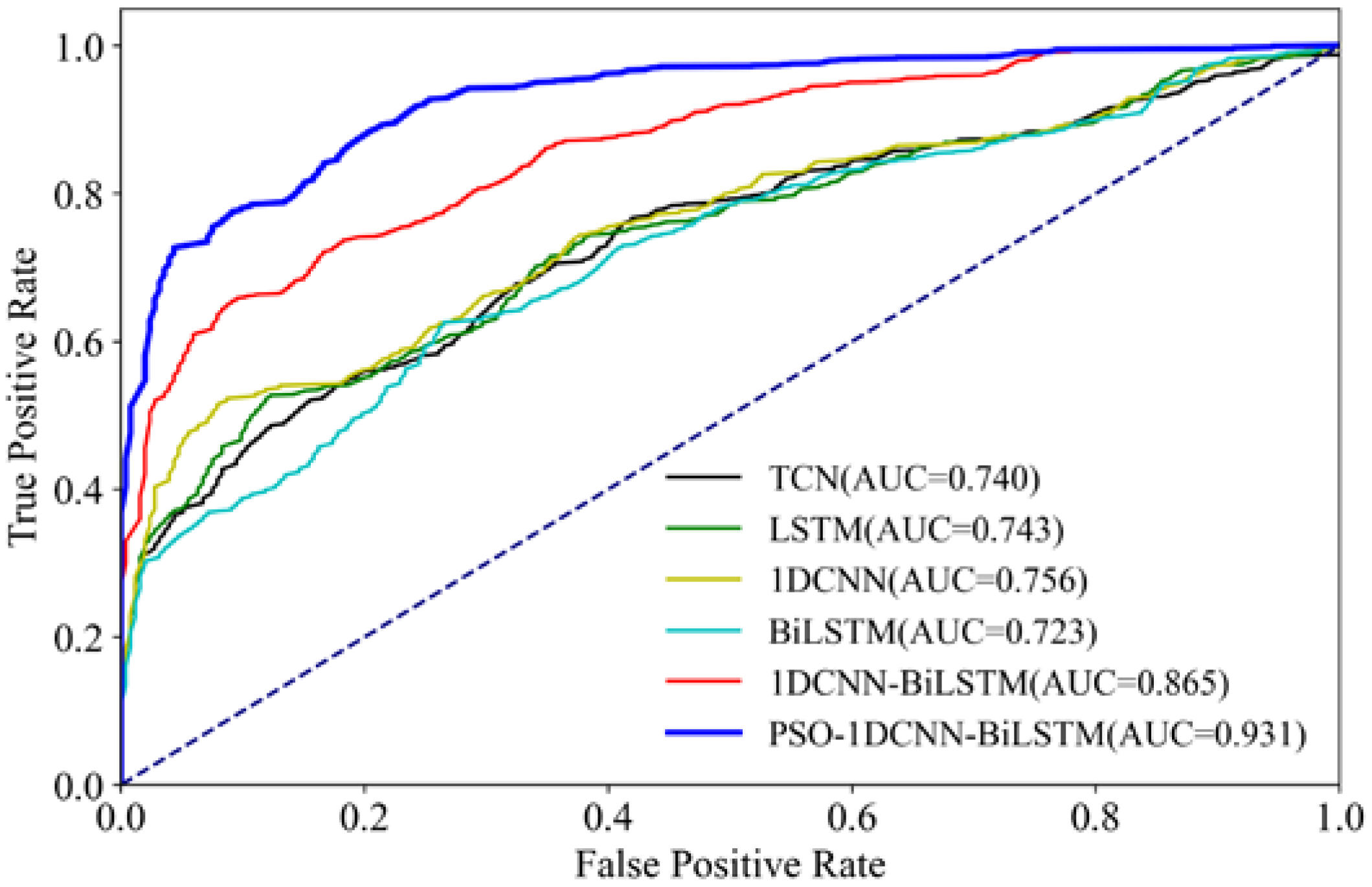
Figure 1. Basic CNN structure.
Information 13 00450 g001
Figure 2. LSTM cell.
Information 13 00450 g002
Figure 3. Functional diagram of BiLSTM.
Information 13 00450 g003
Figure 4. Model structure diagram.
Information 13 00450 g004
Figure 5. Algorithm flow chart.
Information 13 00450 g005
Figure 6. Model convergence performance during the training phase.
Information 13 00450 g006
Figure 7. ROC curve.
Information 13 00450 g007
Figure 8. KS curve.
Figure 8. KS curve.
Information 13 00450 g008
Table 1. Results of Testing Models.
MethodAccuracyKappaRecallPrecisionF1G-meanAUC
TCN0.8060.8270.9710.8510.9070.7030.740
LSTM0.6940.7460.9530.7830.8600.6140.743
1DCNN0.7790.7950.9660.8360.8970.6800.756
BiLSTM0.8160.8190.9790.8510.9110.7100.723
1DCNN-BiLSTM0.8970.9020.9770.9280.9430.8670.865
PSO-1DCNN-BiLSTM0.9210.9190.9780.9480.9540.8960.931
Publisher’s Note: MDPI stays neutral with regard to jurisdictional claims in published maps and institutional affiliations.

