Article

An Intrusion Detection Method for Industrial Control System Based on Machine Learning

School of Artificial Intelligence and Data Science, Hebei University of Technology, Tianjin 300132, China
*
Author to whom correspondence should be addressed.
Information 2022, 13(7), 322; https://doi.org/10.3390/info13070322
Submission received: 7 June 2022 / Revised: 30 June 2022 / Accepted: 1 July 2022 / Published: 3 July 2022
(This article belongs to the Special Issue Advances in Computing, Communication & Security)

Abstract

:
The integration of communication networks and the internet of industrial control in Industrial Control System (ICS) increases their vulnerability to cyber attacks, causing devastating outcomes. Traditional Intrusion Detection Systems (IDS) largely rely on predefined models and are trained mostly on specific cyber attacks, which means the traditional IDS cannot cope with unknown attacks. Additionally, most IDS do not consider the imbalanced nature of ICS datasets, thus suffering from low accuracy and high False Positive Rates when being put to use. In this paper, we propose the NCO–double-layer DIFF_RF–OPFYTHON intrusion detection method for ICS, which consists of NCO modules, double-layer DIFF_RF modules, and OPFYTHON modules. Detected traffic will be divided into three categories by the double-layer DIFF_RF module: known attacks, unknown attacks, and normal traffic. Then, the known attacks will be classified into specific attacks by the OPFYTHON module according to the feature of attack traffic. Finally, we use the NCO module to improve the model input and enhance the accuracy of the model. The results show that the proposed method outperforms traditional intrusion detection methods, such as XGboost and SVM. The detection of unknown attacks is also considerable. The accuracy of the dataset used in this paper reaches 98.13%. The detection rates for unknown attacks and known attacks reach 98.21% and 95.1%, respectively. Moreover, the method we proposed has achieved suitable results on other public datasets.

1. Introduction

The early Industrial Control System (ICS) was relatively independent and rarely connected to the external Internet, which made ICS mainly focus on the availability and rapidity of the system, ignoring security. Therefore, the ICS is vulnerable to attacks from the external internet [1]. Although there have been many studies on the detection methods of known attack traffic in historical network traffic, with the emergence of unknown attacks in the external internet, it is difficult to ensure the security of ICS only by detecting known attacks [2]. In addition, the attack traffic generally only accounts for a small part of all traffic in ICS, and the uneven distribution or imbalance of the data also makes it difficult to establish an intrusion detection model [3]. Therefore, it is crucial to efficiently detect unknown attacks and develop a model for imbalanced data in the ICS.
Intrusion detection methods are mainly divided into misuse-based and anomaly-based intrusion detection methods [4]. Misuse-based intrusion detection methods detect attack traffic in ICS by comparing the feature of detected traffic with the known attack traffic of historical traffic. A misuse-based model, such as Snort [5], can efficiently detect known attacks with a low False Positive Rate (FPR), but it cannot identify unknown attacks. Anomaly-based intrusion detection methods detect attack traffic in ICS by comparing the detected network traffic with normal network traffic. The anomaly-based model [6] can detect all anomaly traffic, including known and unknown attacks. However, it has a high FPR and cannot classify attacks by the feature of attack traffic.
The isolation forest algorithm [7] has become one of the most commonly used algorithms for early intrusion detection due to its simplicity and rapidity. However, it can only filter out outliers, which cannot meet the requirements of the increasingly complex ICS environment. In recent years, the heuristic intrusion detection method [8] has become more and more popular as an anomaly-based intrusion detection method. It detects attack traffic by monitoring and learning normal activities and events on the ICS [9,10,11]. The more patterns it learns about normal activities and events, the more accurately it can detect anomaly activities and events. Prasath [12] presented a heuristic algorithm for intrusion detection in SDN networks. This method is focused on finding anomalies using extracted features of flows, e.g., duration, protocol type, service. Mukhopadhyay et al. [13] proposed a lightweight heuristic intrusion detection and prevention system; its decision-making engine is based on frame data and source/destination addresses.
In addition, there are many common intrusion detection algorithms. Azeroual and Nikiforova proposed an intrusion detection method based on the big data analysis engine Apache Spark, which implements intrusion detection in Sparks MLlib through the k-means algorithm [14]. The k-means algorithm relies on the extraction of feature variables. When there is a lot of noise in the dataset, it is difficult for k-means algorithm to achieve good results. Muhuri and Chatterjee developed a new method for intrusion detection to classify the IDS dataset by combining a genetic algorithm for optimal feature selection and LSTM with an RNN [15]. Xiao, Y. and Xiao, X. proposed a simplified residual network (S-ResNet), which consists of several cascaded and simplified residual blocks. S-ResNet optimizes the problem that residual networks (ResNets) tend to overfit to low-dimensional and small-scale datasets [16]. However, compared with machine learning, the number of parameters and the size of the dataset required for deep learning are considerable, which significantly increases the training cost. Zheng and Hong proposed an improved linear discriminant analysis method based on extreme learning machine (ELM) classification for intrusion detection. This method improves linear discriminant analysis (LDA) and then uses it to reduce feature dimensions [17]. However, such methods cannot detect unknown attacks. SVM and OCSVM are also common intrusion detection algorithms. SVM [18] and OCSVM [19] are similar in that they cannot detect the attack category.
To address the limitations of misuse-based and anomaly-based intrusion detection methods and imbalanced training samples, we propose the NCO–double-layer DIFF_RF–OPFYTHON intrusion detection method for ICS. First, we propose the normal_DIFF_RF–OPFYTHON method. The first step of normal_DIFF_RF–OPFYTHON uses the DIFF_RF module, quickly filtering out anomaly traffic by comparing the detected network traffic with the normal traffic. This step makes the following OPFYTHON module no longer fit a large amount of normal traffic, because the normal traffic has been filtered by the normal_DIFF_RF module, which solves the imbalance of the training samples. The second step uses the OPFYTHON module to compare the filtered anomaly traffic with the known attack traffic. In this step, the filtered anomaly traffic is classified according to feature of attack traffic, which solves the problem that the first step can only detect the attack traffic but cannot classify it by its features.
There are two types of problems in the above normal_DIFF_RF–OPFYTHON:
(i) The accuracy of the model is largely affected by the accuracy of normal_DIFF_RF.
(ii) It is unable to identify unknown attacks. When unknown attack traffic appears in the detected network traffic, the unknown attack traffic will be classified into the most similar known attack traffic by the OPFYTHON.
In this paper, we focus on the above two types of problems to improve the normal_DIFF_RF–OPFYTHON intrusion detection method and propose the NCO–double-layer DIFF_RF–OPFYTHON intrusion detection model as the final model. By analyzing the experimental results, the method solves the imbalance of training samples. The accuracy and the detection rate of unknown attacks reach 98.7% and 98.21%, respectively.
The rest of this paper is organized as follows. Section 2 reviews the related work and some algorithms. Section 3 discusses the dataset preparation, the evaluation metrics of the final model, and experimental results. Finally, conclusions are drawn in Section 4.

2. Materials and Methods

The intrusion detection method we proposed consists of three modules: the NCO module, the double-layer DIFF_RF module, and the OPFYTHON module. It mainly includes the following five steps:
(1) Preprocessing the original ICS network traffic data, including converting categorical variables to numeric variables, normalization, and splitting the data.
(2) Using the NCO algorithm to optimize the input structure of the double-layer DIFF_RF module.
(3) Training the double-layer DIFF_RF module and the OPFYTHON module with the training set.
(4) Integrating the NCO module, the double-layer DIFF_RF module, and the OPFYTHON module to obtain a complete intrusion detection model (NCO–double-layer DIFF_RF–OPFYTHON) and optimize the parameters.
(5) Using the testing set to prove the feasibility, reliability, and superiority of the method we proposed.
The complete structure of the intrusion detection method is shown in Figure 1.

2.1. Normal_DIFF_RF–OPFYTHON Model

There is often an imbalance of data in the network traffic of ICS. The imbalance of training samples will significantly affect the accuracy of the model. In this section, we propose the normal_DIFF_RF–OPFYTHON detection model. It uses the binary classification normal_DIFF_RF [20] module to filter the attack traffic in the detected network traffic firstly, and then uses the multi-classification OPFYTHON [21] module to classify the attack traffic. In this way, the OPFYTHON module does not need to fit a large of normal traffic during the training phase, and solves the imbalance of datasets caused by a large of normal network traffic.

2.1.1. DIFF_RF Algorithm

The DIFF_RF algorithm builds a model by fitting the traffic of the same label to determine whether the detected network traffic belongs to this label. For example, during the training phase, DIFF_RF only fits the normal network traffic among all the network traffic. In the testing phase, it is judged whether the detected network traffic is normal network traffic.
The training phase of the DIFF_RF module needs to set two meta-parameters: Ψ, the number of subsets S randomly drawn from training samples, and t, the number of trees in the forest. The DIFF_RF F = { T ( S 1 ) , T ( S 2 ) , T ( S t ) } consists of { S 1 , S 2 , S t } randomly drawn. Dimensions with high entropy can be assimilated to noise, so the DIFF_RF algorithm prefers to use medium-low entropy input variables to train the model. In order to obtain the entropy of each input variable, the DIFF_RF will calculate the entropy of all input variables by histogram. Equation (1) shows the calculation process of the entropy of each input variable, and Equation (2) shows the process of entropy normalization.
Entropy calculation:
E E i = 1 log 2 ( # b i n s ) k = 1 # b i n s b k / | S | · log 2 ( b k / | S | ) i { 1 , 2 , d }
where #bins is the number of bins in the histogram, and S is a subset randomly drawn from the training samples.
Entropy normalization:
H q i = 1 H q / log 2 ( # b i n s ) i { 1 , 2 , d }
where Hq is the entropy of each of input variable.
We constructed a DIFF Tree of each sample using Algorithm 1.
Algorithm 1 Built a DIFF Tree
DIFF_Tree (S, h, hmax)
Input (S: a sample randomly drawn from X n , h: the current depth level,
hmax :   the   maximal   depth   limit ,   empirically   set   up   to   log 2 ψ )
1 :   if   h     h max   or   | S | 1
2: f n = | S | / ψ
3 :   if   | S | 0 :
4: M S = M e a n ( S )
5 :   σ S = s t a n d a r d _ D e v i a t i o n ( S )
6: else:
7 :   M S = N o n e
8 :   σ S = N o n e
9: end if
10: return leafNode (S, MS, σS, f r )
11: else:
12 :   D = g e t _ q D i s t r i b u t i o n ( S )
13: Randomly select a dimension q { 1 , , d } according to distribution D
14: Randomly select a split value P between max and min values along dimension
15 :   S l = f i l t e r ( S , q < p ) ,   S r = f i l t e r ( S , q p )
16: return inNode(Left = DIFF_Tree ( S l , h + 1, h max ),
17: Right = DIFF_Tree (Sr, h + 1, h max ),
18: splitAtt = q, splitVal = p)
19: end if
During the testing phase, the DIFF_RF algorithm classifies the detected network traffic by calculating scores and setting an appropriate threshold parameter. When the score is less than the threshold, the detected traffic is considered to be the same type with training sample. Otherwise, it is considered not to be the same network traffic. Equation (3) shows the process of calculating the score δ T ( x ) of each DIFF tree.
δ T ( x ) = 2 α 1 d i = 1 d ( x ( i ) M S ( i ) σ S ) 2
where M S ( i ) represents the centroid of the i-th input variable in the training samples, x ( i ) represents the value of the i-th input variable in the testing samples, and σ S represents the standard deviation of the training samples.
The DIFF algorithm calculated score is the average mathematical expectation of each tree in the forest. Equation (4) shows the process of calculating the score p w a s ( x ) of DIFF_RF, where E represents the average mathematical expectation.
p w a s ( x ) = E ( δ T ( x ) )

2.1.2. OPFYTHON Algorithm

The OPFYTHON algorithm converts the training set into a complete graph, and the complete graph consists of several nodes and arcs connecting the nodes. Each sample in the training set corresponds to a node in the complete graph, and the arc between the two adjacent nodes corresponds to the distance between the two adjacent nodes. The larger the weight of the arc between the adjacent nodes, the lower the similarity between the two nodes.
During the modeling process, let Z be a dataset composed of training and testing sets denoted as Z1 and Z2, respectively. One can define a graph G = ( V , A ) 3 which belongs to Z such that v ( s ) V , where S stands for a sample in dataset Z and v ( ) stands for a feature extraction function. Additionally, let A be an adjacency relation that connects samples in V, and let chord-distance be a distance function that weighs edges in A. Of course, there are many choices of distance function for the OPFYTHON algorithm, and the chord-distance is just one of them. Equation (5) shows the calculation formula of chord-distance.
c h o r d - d i s t a n c e = 2 2 i = 1 n x i y i i = 1 n x i 2 i = 1 n y i 2
In the training phase, let π S be a path in G that ends in nodes s V and let π S · ( s , t ) be the nexus between path π S and arc ( s , t ) A . The OPF classifier aims at establishing a set of prototype nodes S V using a cost function f defined by Equation (6).
f max ( S ) = { 0 , + , i f   s S o t h e r w i s e f max ( π S s , t ) = max { f max ( π S ) , d ( s , t ) }
where f max ( π S s , t ) is the maximum distance between adjacent samples along the path π S s , t . Thus, its training algorithm minimizes f max for every sample t Z 1 , assigning an optimum path P ( t ) with a minimum cost defined by Equation (7).
C ( t ) = min π t ( Z 1 , A ) { f max ( π t ) }
In the testing phase, each sample t will be connected to a sample s V 1 , becoming part of the original graph. The algorithm’s goal is to find an optimum path P ( t ) that connects a prototype to node t, which is achieved by evaluation of the path through an optimum cost function denoted by Equation (8).
C ( t ) = min s Z 1 { max { C ( s ) , d ( s , t ) } }

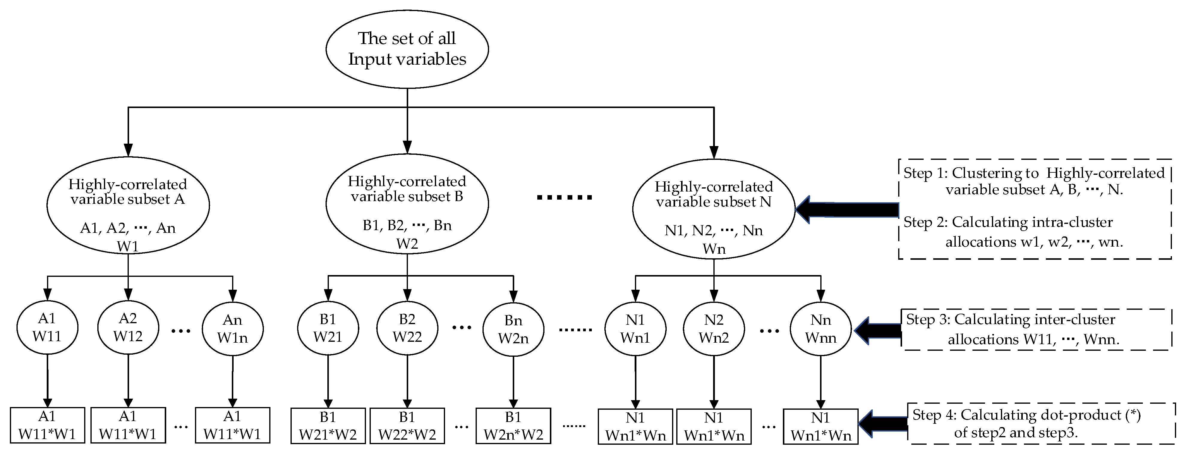
2.2. NCO–Normal_DIFF_RF–OPFYTH Model

As mentioned at the end of the introduction, there are two types of problems in the normal_DIFF_RF–OPFYTHON model.
(i) The accuracy of the model is largely affected by the accuracy of normal_DIFF_RF.
(ii) It is unable to identify unknown attacks.
For the first problem (i), in this section, we improve the DIFF_RF module by nested clustered optimization (NCO) [22] based on the above work. NCO contains the instability within each cluster, and the instability caused by intra-cluster noise does not propagate across clusters. Compared to before the improvement, the NCO–normal_DIFF_RF–OPFYTHON model has a better weight distribution of input variables, and it reduces the prediction error of the model.
Certain covariance structures in the input variables can increase the prediction error of the model. For example, assuming the correlation matrix between two variables is C, the matrix C can be diagonalized as C W = W Λ , where:
C = [ 1 ρ ρ 1 ] , Λ = [ 1 + ρ 1 ρ ] , W = [ 1 2 1 2 1 2 1 2 ]
Inverse C to derive C 1 .
C 1 = W Λ 1 W = 1 | C | [ 1 ρ ρ 1 ]
where | C | = Λ 1 , 1 Λ 2 , 2 = ( 1 + ρ ) ( 1 ρ ) = 1 ρ 2 . From the above, we can see that the correlation coefficients deviating from 0 will cause | C | to approach 0, which makes the values of C 1 explode. In the training phase, this signal structure will increase the prediction error of the model.
The processing steps of the NCO algorithm are as follows:
(1) Clustering all input variables into subsets of highly correlated variables by a hierarchical method.
(2) Calculating optimal allocations for each of these subsets of highly correlated variables separately.
(3) Calculating optimal allocations for each of the variables in all subsets of highly correlated variables.
(4) Calculating the dot product of the intra-cluster allocations (step 2) and the inter-cluster allocations (step 3) to obtain the final optimal allocation.
The flow chart of the NCO is shown in Figure 2.

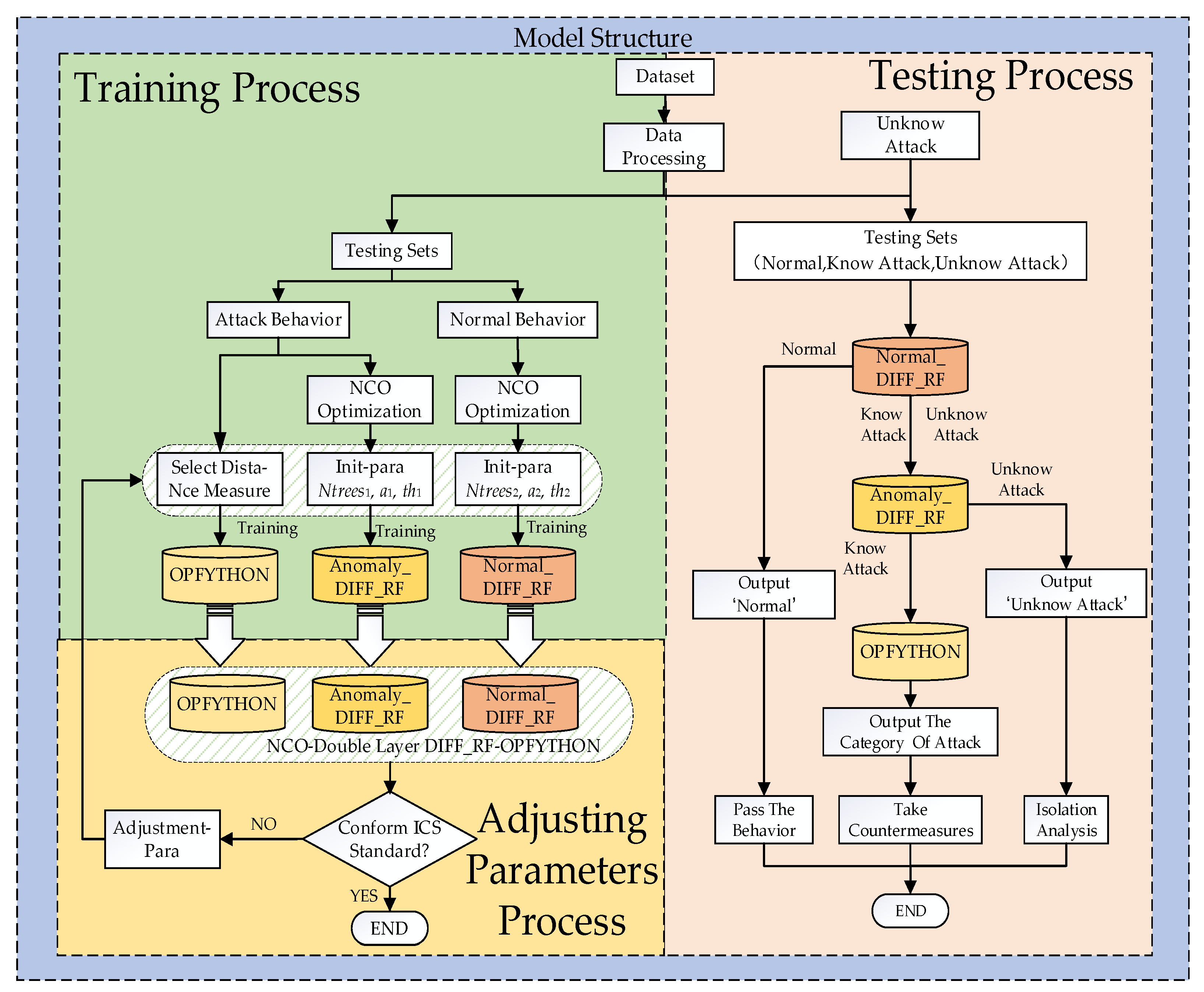
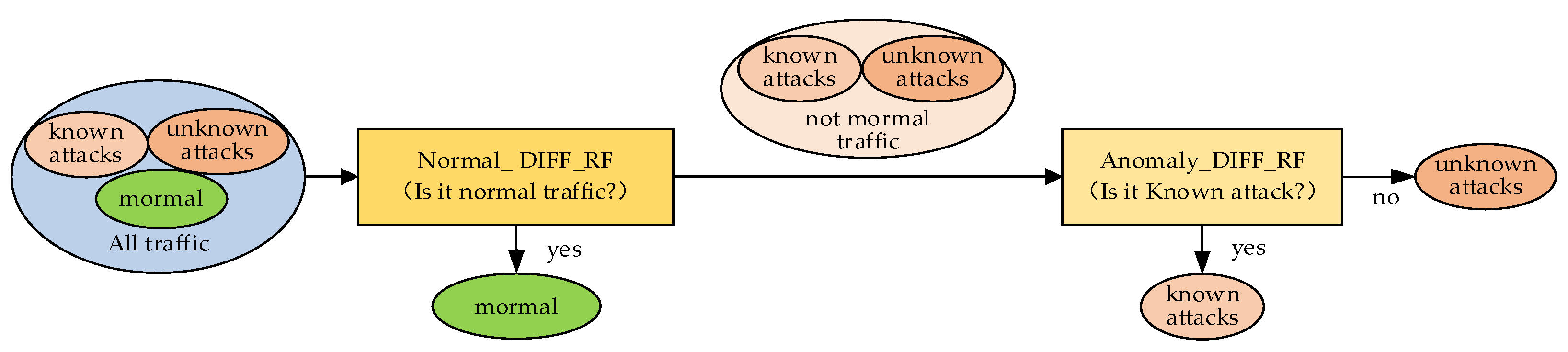
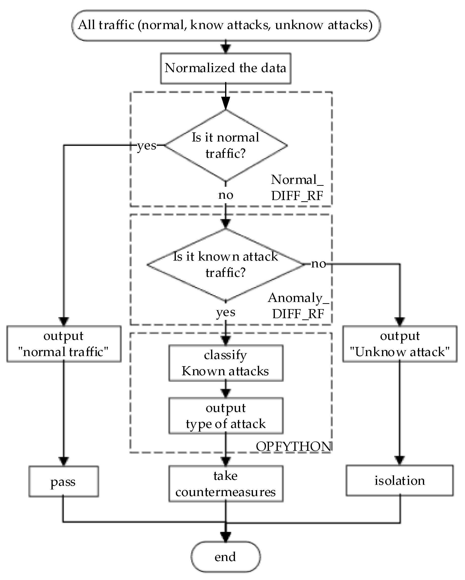
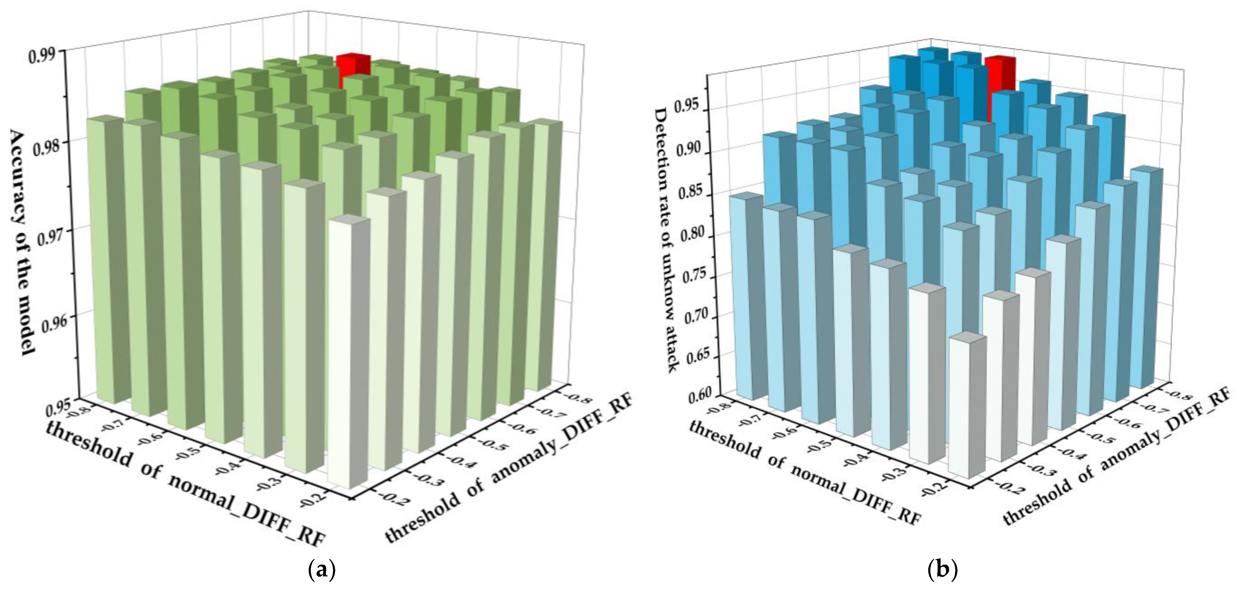
2.3. NCO–double-layer DIFF_RF–OPFYTHON Model

A second problem remains in the NCO–normal_DIFF_RF–OPFYTHON.
(ii) It is unable to identify unknown attacks. When unknown attack traffic appears in the detected network traffic, the unknown attack traffic will be classified into the most similar known attack traffic by the OPFYTHON module.
For problem (ii), in this section, we improve the model structure based on the above work. Finally, we propose the NCO–double-layer DIFF_RF–OPFYTHON method. It adds a layer of anomaly_DIFF_RF module to the NCO–normal_DIFF_RF–OPFYTHON model. During the training phase, anomaly_DIFF_RF only fits the known attack traffic among all the network traffic. In the testing phase, it is judged whether the detected network traffic is known attack traffic. The anomaly_DIFF_RF module can only determine whether the detected network traffic is a known attack, which means that it can only classify the detected network traffic into two categories: belonging or not belonging to known attacks. That is to say, the anomaly_DIFF_RF module will classify both normal network traffic and known attack traffic as not unknown attack traffic. However, before the anomaly_DIFF_RF module, the normal_DIFF_RF module will classify the detected network traffic as belonging or not belonging to normal network traffic. By establishing the double-layer DIFF_RF module, consisting of the normal_DIFF_RF module and the anomaly_DIFF_RF module, the detected network traffic is divided into three categories: normal traffic, known attacks, and unknown attacks.
The flow of the double-layer DIFF_RF module is shown in Figure 3.
After the above step-by-step improvement, the final NCO–double-layer DIFF_RF–OPFYTHON model solves the following three problems.
(i) Imbalanced training samples caused by excessive normal network traffic.
(ii) Low accuracy caused by DIFF_RF module.
(iii) Inability to identify unknown attacks.
The complete detection process of the final NCO–double-layer DIFF_RF–OPFYTHON model is shown in Figure 4.

3. Results

3.1. Dataset Description

The dataset used in this paper is the network traffic in the real ICS collected by Wireshark. The dataset contains 92,272 network traffic data points, including 57,693 normal network traffic data points and 34,579 attack traffic data points. There are five categories of attacks in the 34,579 attack traffic data points. In order to improve the quality of the dataset, we preprocessed the above original dataset by deleting data with missing values, randomly extracting data to reduce the amount of data, etc. The data distribution of the preprocessed valid dataset used in this paper is shown in Table 1.
Category is the category of traffic, including natural traffic and five kinds of attack traffic; Label is the class label; Count is the statistical quantity of each category; and Imbalance is the imbalance coefficient (the ratio of large sample class to small sample class) [23].
In order to test the detection ability of unknown attacks, we regard 500 groups of scapy attacks as unknown attacks, and they do not participate in the training phase. Labels 0–4 in the dataset are divided into the training set and the testing set according to the ratio of 2:1. Label 5 in the dataset is added to the testing set. The training set mentioned above is used to train the NCO–double-layer DIFF_RF–OPFYTHON model, and the testing set is used to test the reliability of the model.

3.2. Evaluation Metrics

The most significant indicator that quantitatively evaluates the performance of the proposed architectures is the (Accuracy, Acc) metric, defined as follows [24]:
A c c = T P + T N T P + T N + F P + F N
where True Positives (TP) indicate the number of anomaly measurements that are identified as anomaly, False Positives (FP) denote the number of normal records that are identified as anomaly, True Negatives (TN) correspond to the number of normal records that are identified as normal, and False Negatives (FN) denote the number of anomaly measurements that are characterized as normal. The confusion matrix [25] is shown in Table 2.
Additionally, we selected the False Positive Rate (FPR) and False Negative Rate (FNR) as evaluation metrics to determine the degree of separability among the different categories since it measures the classification performance of positive and negative. FNR and FPR scores close to 0 indicate highly robust models that can determine the different classes. Moreover, we exploit the Precision, Recall, and F1-score metrics defined as follows [26]:
P r e c i s i o n = T P T P + F P , R e c a l l = T P T P + F N , F 1 - s c o r e = 2 T P 2 T P + F P + F N
A high score on the Precision metric indicates a lower False Positive Rate, i.e., achieving less fault-free data that were incorrectly marked as faulty. On the other hand, a high score on the Recall metric demonstrates low ratio of False Negatives, and thus prevents false event detection. F1-score provides the harmonic mean of Precision and Recall by capturing these two measures in a single metric. Finally, in order to test the classification ability of different attacks, including known and unknown attacks, we use the Detection Rate (DR) as another evaluation metric for model evaluation. DR reflects the ability of the model to classify abnormal samples, which is defined as follows [27]:
D R = T P T P + F N

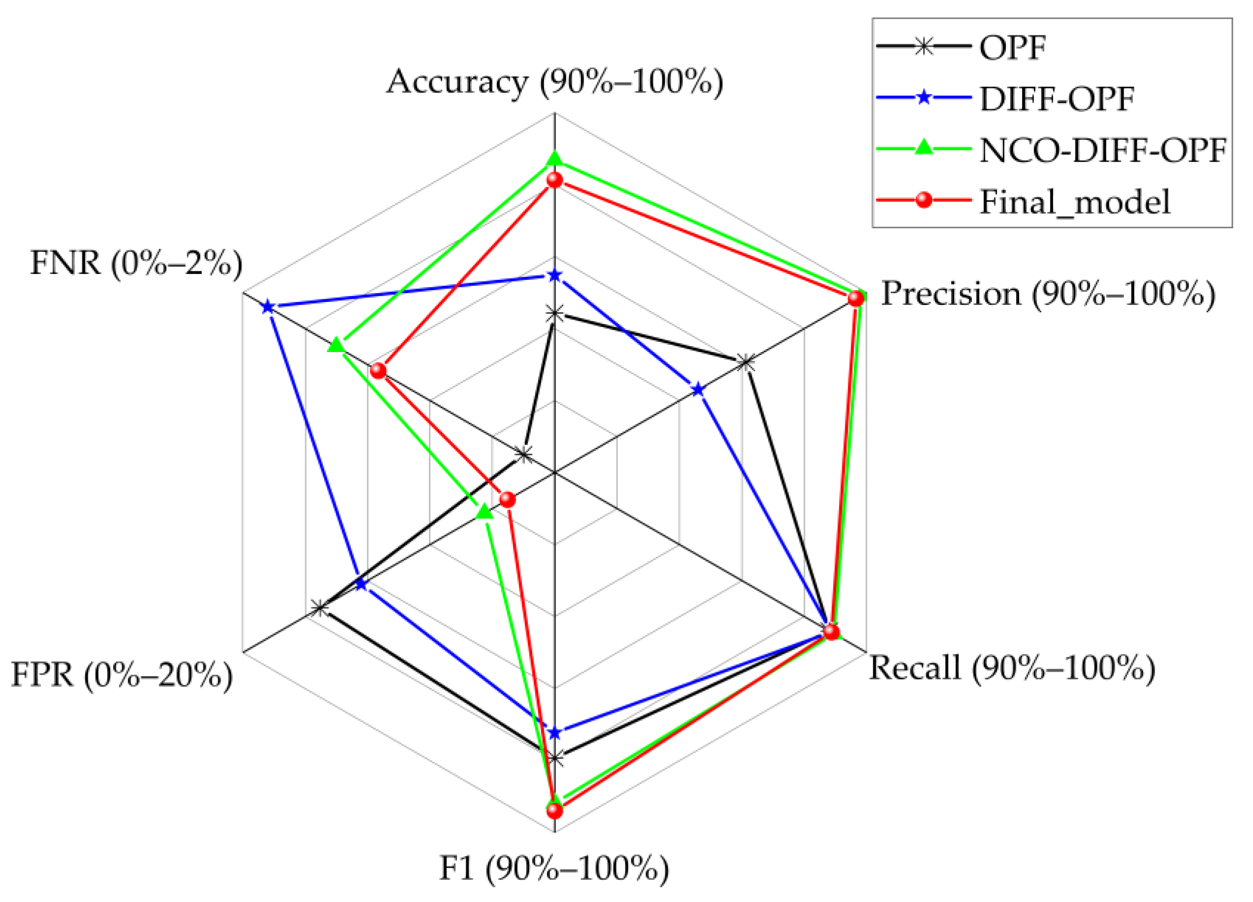
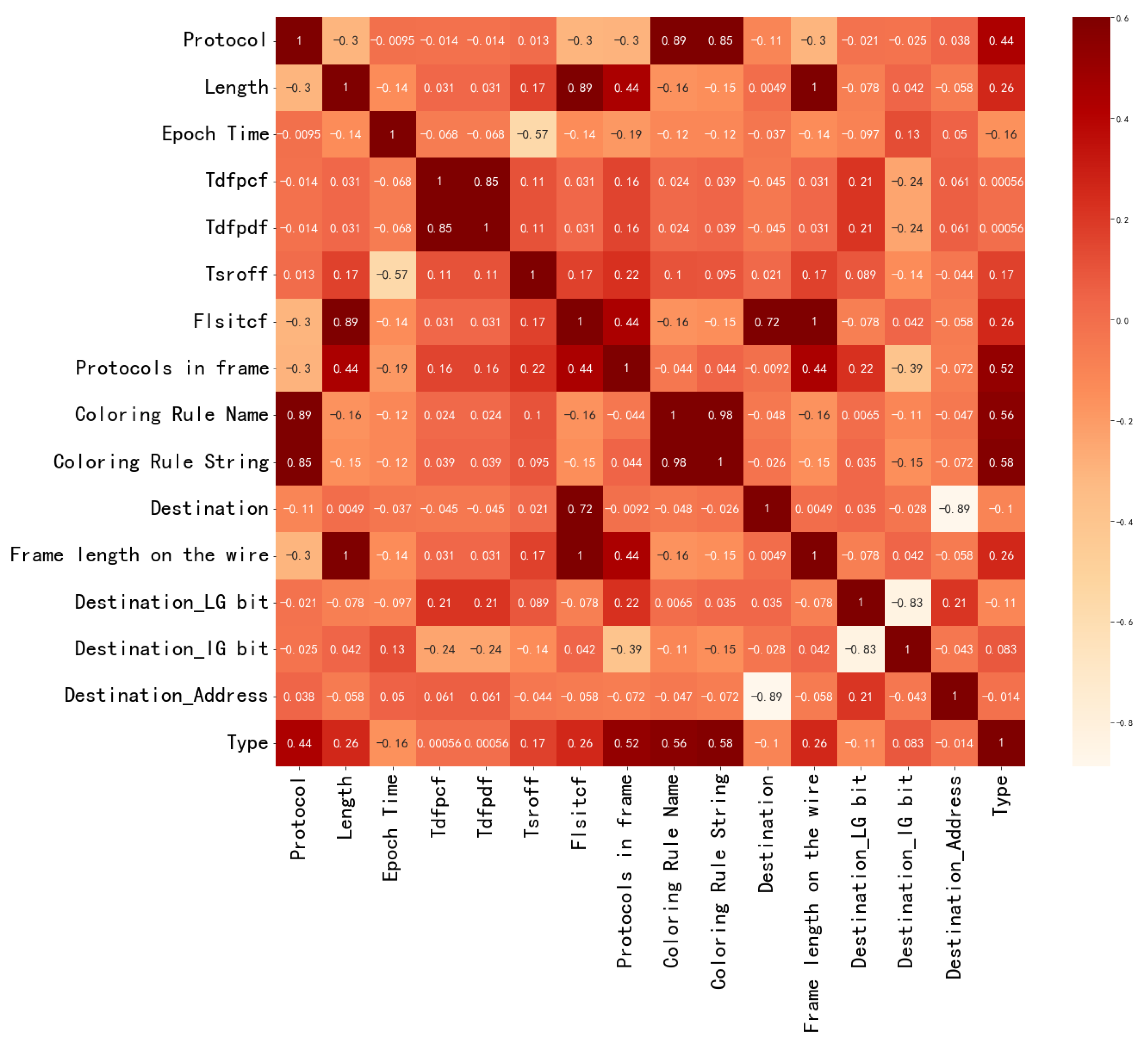
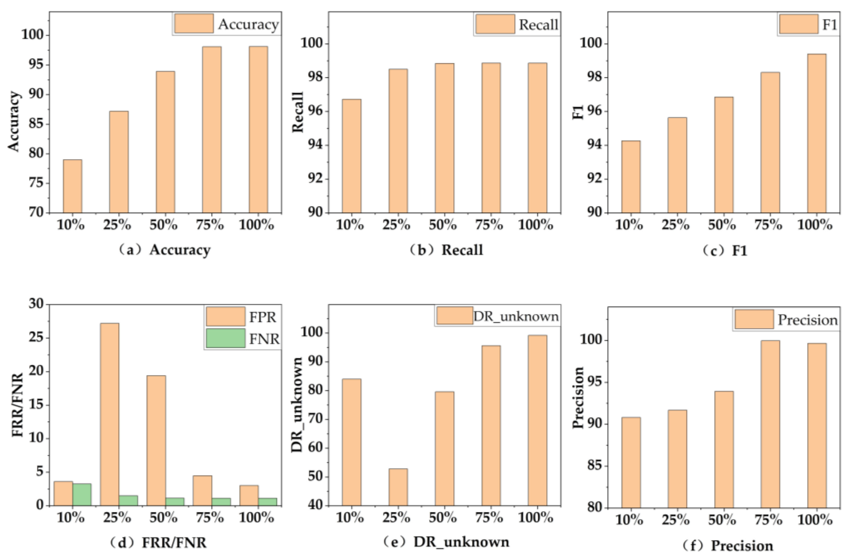
3.3. Experimental Results

In the following paragraphs, we demonstrate the evaluation results obtained using the proposed formulations: (i) NCO–normal_DIFF–OPFYTHON for some situations without unknown attacks, and (ii) NCO–double-layer DIFF_RF–OPFYTHON for some situations with unknown attacks. Regarding the dataset split, we follow a 66.7–33.3% split ratio for both architectures, considering 66.7% of our dataset for the training phase, and 33.3% for the testing phase. Since we are dealing with real-world data that are highly incomplete, we preprocess the raw data to ensure the validity of the dataset.
As mentioned in Section 2.1.1, the DIFF_RF algorithm needs to set two threshold parameters as hyper-parameters for the NCO–double-layer DIFF_RF–OPFYTHON model. Appropriate parameters can make the model perform better. Therefore, in Figure 5, we show the Acc and DR_unknown of the NCO–double-layer DIFF_RF–OPFYTHON model under different threshold parameters. It is worth mentioning that the DIFF_RF module classifies the network traffic by calculating the score and comparing it with the threshold parameter, and since the score calculated by the DIFF_RF module is normalized to [−1,0], the value of the threshold parameter is set to [−1,0].
In Figure 5a, the x-axis represents the threshold parameter of the normal_DIFF_RF module, the y-axis represents the threshold parameter of the anomaly_DIFF_RF module, and the z-axis represents the accuracy of the model on the testing sets, which includes known attacks and unknown attack traffic. The darker the color of the column, the higher the accuracy of the model, and the red column is the column with the highest accuracy. As we can see, when the threshold parameter of the normal_DIFF_RF module is −0.6 and the threshold parameter of the anomaly_DIFF_RF module is −0.7, the model has the highest classification accuracy on the testing set, including known attacks and unknown attacks, and the accuracy reaches 98.7%. Under the same parameters, the detection rate of unknown attacks (in this experiment, we use 500 groups of scapy attacks as unknown attack traffic) reaches 97.8%.
In Figure 5b, the x-axis and y-axis are the same as the Figure 5a, and the z-axis represents the detection rate of unknown attacks. The darker the color of the column, the higher the detection rate of unknown attack of the model, and the red column is the column with the highest detection rate of unknown attack. When the threshold parameter of the normal_DIFF_RF module is −0.8, and the threshold parameter of the anomaly_DIFF_RF module is −0.6, the model has the highest detection rate for unknown attacks, which reaches 98.21%. Under the same parameters, the accuracy of the model reaches 98.39%.
Although the highest accuracy reaches 98.7% and the highest detection rate of unknown attacks reaches 98.21%, we can find that the threshold parameters of both are different, which means that the accuracy and the detection rate of unknown attacks cannot be optimal under the same threshold parameters. In engineering applications, it is necessary to make flexible choices according to the actual situation.
Figure 6 shows the results of OPFYTHON, normal_DIFF_RF–OPFYTHON, NCO– normal_DIFF_RF–OPFYTHON, and NCO–double-layer DIFF_RF–OPFYTHON on the dataset we used in this paper. Since only the NCO–double-layer DIFF_RF–OPFYTHON model can detect unknown attacks, in order to ensure the fairness of the experimental process, the testing set of the experiment shown in Figure 6 eliminates the unknown attacks.
Figure 6 shows six evaluation metrics for different intrusion detection methods, and the content in brackets after the evaluation metrics is the start and end of the axis scale. Figure 6 shows that of the four intrusion detection methods, the NCO–normal_DIFF_RF–OPFYTHON model has the best performance in detecting known attacks. The final model NCO–double-layer DIFF_RF–OPFYTHON has an extra layer of anomaly_DIFF_RF module compared to normal_NCO–DIFF_RF–OPFYTHON. The anomaly_DIFF_RF module cannot achieve 100% accuracy, resulting in the accuracy and other evaluation metrics of NCO–double-layer DIFF_RF–OPFYTHON being inferior to normal_NCO–DIFF_RF–OPFYTHON. In other words, the NCO–double-layer DIFF_RF–OPFYTHON model sacrifices part of its performance to achieve the detection of unknown attacks. Another point to address in Figure 6 is that the OPF model has the best performance on the FNR evaluation metrics, because the OPF model is a misuse-based intrusion detection model. In contrast, others are mixed misuse- and anomaly-based models.
The high correlation between the input variables will affect the training effect of the model. A heatmap of the correlation coefficients of input variables [28] is shown in Figure 7. In the heatmap, the correlation coefficient of each two input variables is in the corresponding position, and the darker the color of A, the stronger the correlation between the two input variables. We can see that the correlation coefficients of some input variables exceed 0.7, which will have adverse effects on modeling [29]. However, the NCO module solves the problem of high correlation between the input variables by optimizing the signal structure of the input variables. As mentioned in Section 2.2, it clusters all input variables into subsets of highly correlated variables, and calculates the optimal allocations for each intra-cluster and inter-cluster. At last, it calculates the dot product of the intra-cluster allocations and the inter-cluster allocations to obtain the final optimal allocation.
In order to verify the superiority of the method we proposed, Table 3 shows the comparison results between the intrusion detection method we proposed and other traditional intrusion detection methods [30,31,32,33]. The conventional machine learning algorithm is supervised learning and cannot detect unknown attacks. In order to ensure the fairness of the experimental process, the testing set in Table 3 eliminates the unknown attacks.
Based on Table 3, the NCO–normal_DIFF_RF–OPF model is significantly better than other conventional intrusion detection models in different evaluation metrics, especially in the detection rate of various attacks. The performance of the NCO–double-layer DIFF_RF–OPFYTHON model is slightly lower than NCO–normal_DIFF_RF–OPFYTHON, but it can detect unknown attacks.
Figure 8 shows the different evaluation metrics of the NCO–double-layer DIFF_RF–OPFYTHON model on datasets of different sizes.
Figure 8 shows seven evaluation metrics of the model we proposed on datasets of different sizes, including 10%, 25%, 50%, 75% and 100%. In Figure 8, we can see that the dataset size of 10% outperforms 25% and 50% on some evaluation metrics. There is a random function in the double-layer DIFF_RF module, which has a random effect on the experimental results. When the size of the datasets is too tiny, this random phenomenon will be more obvious. However, with the increase in the size of the datasets, although this random phenomenon also exists, it will have less of an impact on the experimental results. This resembles a coin toss experiment—maybe the distribution of the results of ten experiments will be uneven, but with the increase in the number of experiments, the distribution of experimental results will stabilize to 50%.
With the increase in the size of the datasets, the evaluation metrics of the NCO–double-layer DIFF_RF–OPFYTHON model are also improving, which is reasonable in the real world. When the size of the datasets is increased from 10% to 75%, the accuracy, FPR, F1, and Precision of the model are significantly improved. However, we can see that when the size of the datasets is about 75%, the evaluation metrics of the model are only slightly less than 100%, which means that the training cost of the model can be reduced by appropriately reducing the size of the datasets when the model does not require the ultimate detection accuracy.
In order to verify the reliability of the intrusion detection method we proposed, the method is also applied to other public datasets, including the University of Mississippi natural gas pipeline datasets [34] and CIC-IDS-2017 datasets [35]. In the experiments on the pipeline dataset, we set the NMRI attacks as unknown attacks to test the detection rate of the unknown attacks. The NMRI attacks only participate in the testing phase and do not participate in any training phase. In the experiments on the CIC-IDS-2017 dataset, we set the bot attacks as unknown attacks to test the detection rate of the unknown attacks. The bot attacks only participate in the testing phase and do not participate in any training phase. Table 4 shows the results of our proposed ICS intrusion detection method on pipeline datasets, CIC-IDS-2017 datasets, and the datasets used in this paper.
According to Table 4, the intrusion detection method we proposed has considerable evaluation metrics on different datasets. The method can efficiently identify known attacks that exist in the training set and unknown attacks that do not exist in the training set.

4. Conclusions

In this study, we examined the performance of efficient and robust intrusion detection methods based on machine learning, namely, NCO–double-layer DIFF_RF–OPFYTHON, for the challenging problem of imbalanced training samples and the inability to detect unknown attacks. The method was trained on its own dataset and two public datasets and simulates scenarios of unknown attacks by making particular partitions of the datasets. The proposed intrusion detection method presents high-quality results regarding the classification accuracy, the function of detecting unknown attacks, and the evaluation metrics compared to state-of-the-art intrusion detection methods. The superiority of the proposed intrusion detection method is evidenced in the fact that it presents high detection accuracy, resolves the imbalance of training samples in the real world, and resolves the problem that the intrusion detection method based on supervised learning cannot detect unknown attacks. The accuracy and the detection rate of unknown attacks of the method reach 98.7% and 98.21%, respectively, which is a satisfactory experimental result.
In terms of future work, there are a few directions worth exploring. In this paper, for example, the basis classifier modules are shallow machine learning algorithms. This can be improved by using a more powerful neural network architecture. In addition, in this study, all the detected unknown attacks are marked as one category. In future work, the unknown attacks can be clustered and analyzed to further classify the detected unknown attacks. It is worth pointing out that the number of unknown attacks is only a small fraction after all, so it is difficult to further classify unknown attacks by cluster analysis. Since training a more powerful neural network requires a lot of data, it is important to explore how to train a new model when the number of samples belonging to this class is limited.

Author Contributions

Conceptualization, methodology, validation, writing, software, Y.C.; conceptualization, Y.C., X.Z. and K.J.; supervision, funding acquisition, review, Y.C., L.Z. and Z.C. All authors have read and agreed to the published version of the manuscript.

Funding

This research received no external funding.

Institutional Review Board Statement

Not applicable.

Informed Consent Statement

Not applicable.

Data Availability Statement

CIC-IDS-2017 datasets are available at https://www.unb.ca/cic/datasets/ids-2017.html (accessed on 3 June 2022). University of Mississippi natural gas pipeline datasets are available at https://sites.google.com/a/uah.edu/tom-my-morris-uah/ics-data-sets (accessed on 3 June 2022).

Conflicts of Interest

The authors declare no conflict of interest.

References

  1. Hu, Y.; Yang, A.; Li, H.; Sun, Y.; Sun, L. A survey of intrusion detection on industrial control systems. Int. J. Distrib. Sens. Netw. 2018, 14, 1550147718794615. [Google Scholar] [CrossRef] [Green Version]
  2. Liu, H.; Lang, B. Machine Learning and Deep Learning Methods for Intrusion Detection Systems: A Survey. Appl. Sci. 2019, 9, 4396. [Google Scholar] [CrossRef] [Green Version]
  3. Thabtah, F.; Hammoud, S.; Kamalov, F.; Gonsalves, A. Data imbalance in classification: Experimental evaluation. Inf. Sci. 2020, 513, 429–441. [Google Scholar] [CrossRef]
  4. Yang, Z.; Liu, X.D.; Li, T. A systematic literature review of methods and datasets for anomaly-based network intrusion detection. Comput. Secur. 2022, 116, 102675. [Google Scholar] [CrossRef]
  5. Shah, S.A.R.; Issac, B. Performance comparison of intrusion detection systems and application of machine learning to Snort system. Future Gener. Comput. Syst. 2018, 80, 157–170. [Google Scholar] [CrossRef]
  6. Gurina, A.; Eliseev, V.; Gurina, A.; Eliseev, V. Anomaly-Based Method for Detecting Multiple Classes of Network Attacks. Information 2019, 10, 84. [Google Scholar] [CrossRef] [Green Version]
  7. Hariri, S.; Kind, M.C.; Brunner, R.J. Extended Isolation Forest. IEEE Trans. Knowl. Data Eng. 2019, 33, 1479–1489. [Google Scholar] [CrossRef] [Green Version]
  8. Niemiec, M.; Kościej, R.; Gdowski, B. Multivariable Heuristic Approach to Intrusion Detection in Network Environments. Entropy 2021, 23, 776. [Google Scholar] [CrossRef]
  9. Bangui, H.; Buhnova, B. Recent Advances in Machine-Learning Driven Intrusion Detection in Transportation: Survey. Procedia Comput. Sci. 2021, 184, 877–886. [Google Scholar] [CrossRef]
  10. Kilincer, I.F.; Ertam, F.; Sengur, A. Machine learning methods for cyber security intrusion detection: Datasets and comparative study. Comput. Netw. 2021, 188, 107840. [Google Scholar] [CrossRef]
  11. Luo, H.; Shi, K.; Qiao, F.; Li, Y. Intrusion Detection Mechanism Based On Modular Neural Network. In Proceedings of the 2020 2nd International Conference on Machine Learning, Big Data and Business Intelligence (MLBDBI), Taiyuan, China, 23–25 October 2020; pp. 419–423. [Google Scholar]
  12. Prasath, M.K.; Perumal, B. A meta-heuristic Bayesian network classification for intrusion detection. Int. J. Netw. Manag. 2019, 29, e2047. [Google Scholar] [CrossRef]
  13. Mukhopadhyay, I.; Gupta, K.S.; Sen, D.; Gupta, P. Heuristic Intrusion Detection and Prevention System. In Proceedings of the 2015 International Conference and Workshop on Computing and Communication (IEMCON), Vancouver, BC, Canada, 15–17 October 2015; pp. 1–7. [Google Scholar]
  14. Azeroual, O.; Nikiforova, A. Apache Spark and MLlib-Based Intrusion Detection System or How the Big Data Technologies Can Secure the Data. Information 2022, 13, 58. [Google Scholar] [CrossRef]
  15. Muhuri, P.S.; Chatterjee, P.; Yuan, X.; Roy, K.; Esterline, A. Using a Long Short-Term Memory Recurrent Neural Network (LSTM-RNN) to Classify Network Attacks. Information 2020, 11, 243. [Google Scholar] [CrossRef]
  16. Xiao, Y.; Xiao, X. An Intrusion Detection System Based on a Simplified Residual Network. Information 2019, 10, 356. [Google Scholar] [CrossRef] [Green Version]
  17. Zheng, D.; Hong, Z.; Wang, N.; Chen, P. An Improved LDA-Based ELM Classification for Intrusion Detection Algorithm in IoT Application. Sensors 2020, 20, 1706. [Google Scholar] [CrossRef] [PubMed] [Green Version]
  18. Gauthama Raman, M.R.; Somu, N.; Jagarapu, S.; Manghnani, T.; Selvam, T.; Krithivasan, K.; Shankar Sriram, V.S. An efficient intrusion detection technique based on support vector machine and improved binary gravitational search algorithm. Artif. Intell. Rev. 2020, 53, 3255–3286. [Google Scholar] [CrossRef]
  19. Wang, Z.; Cha, Y.-J. Unsupervised deep learning approach using a deep auto-encoder with a one-class support vector machine to detect damage. Struct. Health Monit. 2021, 20, 406–425. [Google Scholar] [CrossRef]
  20. Marteau, P.F. Random Partitioning Forest for Point-Wise and Collective Anomaly Detection—Application to Network Intrusion Detection. IEEE Trans. Inf. Forensics Secur. 2021, 16, 2157–2172. [Google Scholar] [CrossRef]
  21. de Rosa, G.H.; Roder, M.; Papa, J.P. Comparative Study Between Distance Measures On Supervised Optimum-Path Forest Classification. arXiv arXiv:2202.03854.
  22. Prado, M. A Robust Estimator of the Efficient Frontier. SSRN Electron. J. 2019, 10, 2139. [Google Scholar]
  23. Liu, L.; Wang, P.; Lin, J.; Liu, L. Intrusion Detection of Imbalanced Network Traffic Based on Machine Learning and Deep Learning. IEEE Access 2020, 9, 7550–7563. [Google Scholar] [CrossRef]
  24. Fotiadou, K.; Velivassaki, T.-H.; Voulkidis, A.; Skias, D.; Tsekeridou, S.; Zahariadis, T. Network Traffic Anomaly Detection via Deep Learning. Information 2021, 12, 215. [Google Scholar] [CrossRef]
  25. Luque, A.; Carrasco, A.; Martín, A.; de las Heras, A. The impact of class imbalance in classification performance metrics based on the binary confusion matrix. Pattern Recognit. 2019, 91, 216–231. [Google Scholar] [CrossRef]
  26. Mokhtari, S.; Abbaspour, A.; Yen, K.K.; Sargolzaei, A. A Machine Learning Approach for Anomaly Detection in Industrial Control Systems Based on Measurement Data. Electronics 2021, 10, 407. [Google Scholar] [CrossRef]
  27. Zhou, Y.L.; Xie, L.; Pan, H. Research on a PSO-H-SVM-Based Intrusion Detection Method for Industrial Robotic Arms. Appl. Sci.-Basel 2022, 12, 2765. [Google Scholar] [CrossRef]
  28. Zhao, S.; Guo, Y.; Sheng, Q.; Shyr, Y. Advanced heat map and clustering analysis using heatmap3. Biomed. Res. Int. 2014, 2014, 986048. [Google Scholar] [CrossRef] [Green Version]
  29. Hsu, H.H.; Hsieh, C.W. Feature Selection via Correlation Coefficient Clustering. JSW 2010, 5, 1371–1377. [Google Scholar] [CrossRef]
  30. Dhaliwal, S.; Nahid, A.A.; Abbas, R. Effective Intrusion Detection System Using XGBoost. Information 2018, 9, 149. [Google Scholar] [CrossRef] [Green Version]
  31. Tao, P.Y.; Sun, Z.; Sun, Z.X. An Improved Intrusion Detection Algorithm Based on GA and SVM. IEEE Access 2018, 6, 13624–13631. [Google Scholar] [CrossRef]
  32. Panigrahi, R.; Borah, S.; Bhoi, A.K.; Ijaz, M.F.; Pramanik, M.; Kumar, Y.; Jhaveri, R.H. A Consolidated Decision Tree-Based Intrusion Detection System for Binary and Multiclass Imbalanced Datasets. Mathematics 2021, 9, 751. [Google Scholar] [CrossRef]
  33. Zhang, J.; Zulkernine, M.; Haque, A. Random-forests-based network intrusion detection systems. IEEE Trans. Syst. Man Cybern. C Appl. Rev. 2008, 38, 649–659. [Google Scholar] [CrossRef]
  34. Morris, T.H.; Thornton, Z.; Turnipseed, I. Industrial control system simulation and data logging for intrusion detection system research. In Proceedings of the 7th Annual Southeastern Cyber Security Summit, Huntsville, AL, USA, 3–4 June 2015; pp. 3–4. [Google Scholar]
  35. Shukla, A.K. Detection of anomaly intrusion utilizing self-adaptive grasshopper optimization algorithm. Neural Comput. Appl. 2021, 33, 7541–7561. [Google Scholar] [CrossRef]
Figure 1. The structure of the NCO–double-layer DIFF_RF–OPFYTHON model.
Information 13 00322 g001
Figure 2. The flow chart of the NCO.
Information 13 00322 g002
Figure 3. The flow of the double-layer DIFF_RF model.
Information 13 00322 g003
Figure 4. Detection process of the final model.
Information 13 00322 g004
Figure 5. Acc and DR_unknown under different threshold parameters. (a) Acc under different threshold parameters. (b) DR_unknown under different threshold parameters.
Information 13 00322 g005
Figure 6. The results of the four models on experimental dataset l.
Information 13 00322 g006
Figure 7. The heatmap of the correlation coefficients of input variables.
Information 13 00322 g007
Figure 8. The performance of final model on datasets of different sizes.
Information 13 00322 g008
Table 1. The data distribution of the preprocessed valid dataset.
CategoryLabelCountImbalance
Natural030,0001
Arp1200015
DDoS2200015
Socket3200015
Nmap4200015
Scapy550060
Table 2. Confusion matrix.
TrueFalse
PositiveTPFP
NegativeFNTN
Table 3. The results of the method we proposed and traditional methods.
AccPrRecF1FprFnrDr-
Arp
Dr-
DDOS
Dr-
Socket
Dr-
Nmap
Dr-
Unknown
Random Forset92.2191.1799.9395.3536.300.0697.6099.108.2044.80no
Decision Tree90.7499.8598.5999.2215.501.4199.80098.4046.80no
SVM93.4495.2799.8497.5018.600.1699.8098.5051.8026.20no
XGboost93.6396.7798.6097.6812.351.4099.8099.3098.401.60no
NCO–normal_DIFF–OPF98.6899.8298.5599.184.501.4099.8010099.0091.80no
NCO–double-layer DIFF–OPF98.1399.9598.8799.403.201.1397.4099.8097.0086.2098.21
Table 4. The results of the three datasets.
AccPrRecF1FprFnrDr_Known 1Dr_Unknown
Gas pipeline97.9799.3297.5298.411.182.4899.8097.87
CIC-IDS-201796.8299.1995.1897.140.994.8298.3699.40
This paper98.1399.9598.8799.403.201.1395.1098.21
1 The unknown attacks set by pipeline and CIC-IDS-2017 are NMRI and bot, respectively.
Publisher’s Note: MDPI stays neutral with regard to jurisdictional claims in published maps and institutional affiliations.

