A Universal Simulation Framework of Shipborne Inertial Sensors Based on the Ship Motion Model and Robot Operating System

Abstract

A complete virtual test environment is a powerful tool for Autonomous Surface Vessels (ASVs) research, and the simulation of ship motion and shipborne sensors is one of the prerequisites for constructing such an environment. This paper proposed a universal simulation framework of shipborne inertial sensors. A ship motion model considering environmental disturbances is proposed to simulate the six-degrees-of-freedom motion of ships. The discrete form of the inertial sensor stochastic error model is derived. The inertial measurement data are simulated by adding artificial errors to a simulated motion status. In addition, the ship motion simulation, inertial measurement simulation, and environment simulation nodes are implemented based on the computational graph architecture of the Robot Operating System (ROS). The benefit from the versatility of the ROS messages, the format of simulated inertial measurement is exactly the same as that of real sensors, which provides a research basis for the fusion perception algorithm based on visual–inertial and laser–inertial sensors in the research field of ASVs.

1. Introduction

Autonomous vehicles are often unsafe and expensive during the testing phase, which limits the completeness verification of related algorithms in diverse scenarios. This issue is further exacerbated by the fact that the sea trials of autonomous ships are more complex and risky than on-land testing [1]. Therefore, high-fidelity simulation is required in the development of autonomous vehicles [2]. Moreover, simulation is an efficient way to generate experimental data in various scenarios for training and testing the perception, decision-making, control, and end-to-end autonomous driving algorithms [3].

A complete perception unit based on various types of sensors is one of the prerequisites of autonomy, considering a fully autonomous ship is capable of making decisions by itself without the supervision of onboard crews or remote human operators [4]. Autonomous ships are able to perceive the ego-motion state, targets, and environment information by employing multi-sensor fusion algorithms [5]. Especially, different from the motion status of a car constrained by the ground, ships are in a full six-degrees-of-freedom (6 DoF) motion during navigating and when disturbed by winds, ocean currents, and waves. Since shipborne sensors are generally fixedly connected to the hull, sensor information such as camera images or LiDAR point clouds will be affected by the ship motions, which brings challenges to the accuracy and stability of perception algorithms. It follows that the inertial sensor is one of the indispensable shipborne sensors used in target perception [6] and ego-motion state estimation [7]. As far as the ship’s ego-motion state estimation is concerned, the fusion state estimation based on visual–inertial [8] and laser–inertial [9] is more stable and efficient than pure visual [10] and laser [11] methods. Therefore, studying the fusion of ship inertial measurement data with other sensors is vital to the perception unit. Given the above, constructing a virtual test environment is necessary to fully test and verify the multi-sensor fusion perception algorithm for ships. The modeling and simulation of inertial sensors and vehicles are the essential parts to build such an environment [12]. However, the reliability of testing results is highly dependent on the accuracy of simulation models.

Numerous studies focusing on either simulating onboard sensors or building a practical virtual test environment have emerged in recent years. While an exhaustive review of current simulation methods of various sensors is beyond the scope of this paper, we hereby mention some notable recent works that deeply influenced this work.

Gazebo [13] has been a popular simulator for research work related to robotics, and the its plugins expand quickly due to the rapid development of the open-source community of the ROS [14]. In Gazebo, the inertial sensors are simulated based on the physics engine, the noise and bias of the linear accelerations, and angular velocities are additive, whereas the bias is treated as a fixed value that is sampled once at the start of a simulation. Plenty of work focus on the simulation of drones [15], cars [16], and robots [14] in Gazebo; however, the modeling and simulation of ships and shipborne sensors in Gazebo are limited compared with other types of vehicles. A recent representative work of a Gazebo-based ASV simulator is the Virtual RobotX (VRX) extends the Gazebo through the addition of vessel dynamics representations [17]. Another excellent work is the USVsim [18], which implements the physical-based motion model of Unmanned Surface Vehicles (USVs) in Gazebo plugins. However, both the VRX and USVsim focus on the ship hydrodynamic modeling and marine environment simulation, the shipborne sensors are inherited from original Gazebo plugins. In other words, the error modeling of the simulated inertial sensors is exactly the same as the Gazebo as discussed above in their work.

Recently, 3D game engines such as Unity 3D and UE4 (Unreal Engine 4) have also become powerful tools for building virtual test environments for autonomous vehicles due to their practical physics engines and realistic scene modeling. LGSVL [19] is a high fidelity simulator for autonomous driving that has already been applied in Autoware [20] and Apollo [21] projects. The LGSVL simulator was developed based on Unity 3D which provides a basic vehicle dynamics model for the ego vehicle and diverse sensor models. However, the inertial sensor model are directly output noise-free data according to the document. Nevertheless, the users can create their own sensor plugins or integrate external third-party dynamics models into the LGSVL simulator. CARLA [22] is an open simulator aiming to support development, training, and validation of autonomous urban driving systems. This simulator is implemented as an open-source layer over UE4 which enables the addition of future extensions by the community. However, the main application scenario of the simulator is vision-based autonomous driving and simulated sensors are limited to RGB cameras. Similarly, AirSim is an open-source simulator published as a plugin of UE4 that aims to perform virtual tests for autonomous vehicles [3]. The core components of this simulator consist of the environment model, vehicle model, and sensor models, etc. In their work, the onboard gyroscope and accelerometers are modeled by adding white noise and bias drift to the ground truth from the vehicle model. It is worth noting that the graphics card manufacturing giant NVIDIA has published a high-fidelity simulation platform called NVIDIA DRIVE Sim [23]. The platform could provide a large-scale, physically accurate multi-sensor simulation. However, the typical research target is limit to autonomous aerial or ground vehicles, and there is no modeling of ships and marine environment in LGSVL, CARLA, AirSim, and NVIDIA DRIVE Sim.

To summarize, there are numerous researches on vehicle-mounted sensor simulation at this stage, but the research on ship-borne sensor simulation is very limited. In aforementioned work, the error model in the inertial sensors is too simple in Gazebo. Moreover, the description of the modeling method of the ship’s physical motion is relatively sketchy in these works. Although the environmental disturbances are considered in some of the studies, the actual ship measurement data are not used to fully verify the simulation and modeling methods. Inspired by the work above, the main focus of this work is to build a universal simulation framework of the shipborne inertial sensors. The physical-based ship motion model is established, and the ship motion simulation method is presented and verified by onboard measurement data. In addition, the discrete stochastic error models of inertial sensors are derived to generate realistic artificial errors. The shipborne inertial measurement data are simulated based on the ship motion simulation and these error models. Moreover, the ROS is employed to construct the simulation framework considering its universality. In other words, the wide application of the ROS in virtual [16,17] and real marine robotics [24] seamlessly connected the simulation and reality. Consequently, the proposed framework can be easily integrated with the ROS-compatible simulators to provide both the noise-free motion status and realistic shipborne inertial measurement data.

The remainder of the paper is structured as follows: Section 2 describes physical-based ship motion modeling and simulation methods. In addition, the ship motion simulation results are validated by onboard measurement data. Section 3 presents the models of inertial sensors, especially the discrete stochastic error models. The simulation framework of the shipborne inertial sensor and implementation details are presented in Section 4. The limitations are discussed and the paper is concluded in Section 5.

2. Physical-Based Ship Motion Modeling and Simulation

The ship motion simulation is one of the prerequisites to simulate shipborne inertial sensors. In this section, the physical-based ship motion model is constructed. Moreover, the simulation method of ship motion under environmental disturbances is proposed, and validated by onboard measurement data. The detailed content is illustrated as follows:

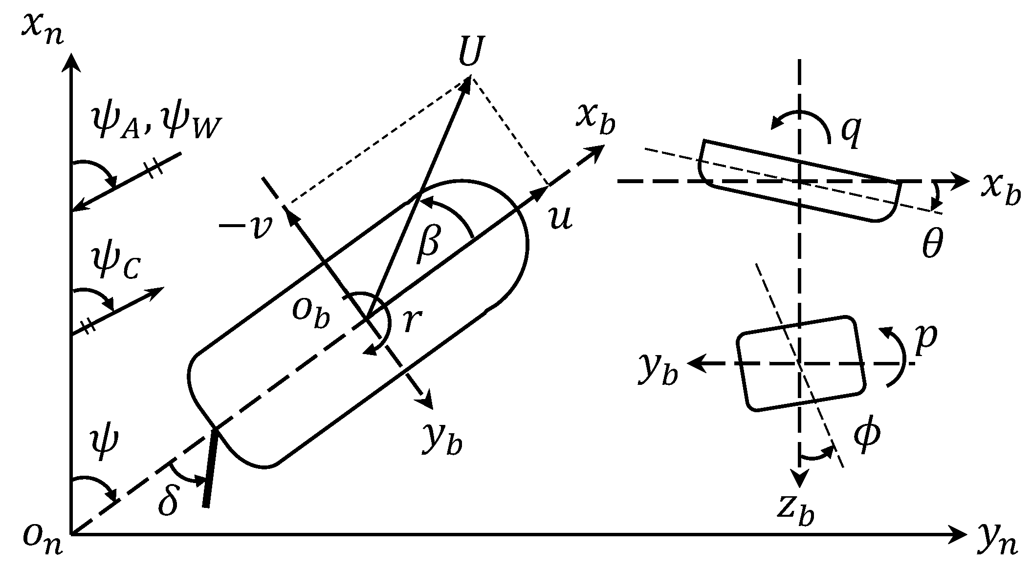
2.1. Physical-Based Ship Motion Model

A bulk carrier was employed in this study and the main particulars of the ship are listed in

Table 1. Main particulars of the bulk carrier.

Items	Value
Length L	160.4 m
Breadth B	27.2 m
Draft d	8.16 m
Propeller type	4-bladed solid × 1 set (FPP)
Propeller diameter DP	5.25 m
Rudder type	Balanced type × 1 set
Rudder area AR	26.4 m2
Sailing speed	14 knots

. This bulk carrier was a tramper that had no regular voyage routes. Moreover, this bulk carrier was equipped with a shipboard measuring system. The data from nautical instruments such as the voyage data recorder (VDR) were well recorded, providing an important data foundation for validating different simulation methods.

The ship motion model was constructed based on rigid body dynamics to perform the 6 DoF motion simulation in the time-domain. The coordinate systems adopted in this paper are shown in Figure 1, where the world frame is denoted by $o_n–x_n{y}_n{z}_n$, and the ship body-fixed frame is denoted by $o_b–x_b{y}_b{z}_b$. Moreover, $U$ in body-fixed frame represents the resultant speed of the ship, which is composed of the heading speed $u$ and lateral speed $v$. The angle between $u$ and $U$ is the so-called drift angle $\beta$. The rudder angle is indicated by $\delta$. Moreover, $\varphi$, $\theta$, and $\psi$ denote the roll, pitch, and yaw angles; $p$,$q$, and $r$ denote the roll, pitch, and yaw angular velocities, respectively. The direction of wind, ocean current, and waves are denoted by ${\psi }_A$, ${\psi }_C$, and ${\psi }_W$ respectively.

According to the vector representation form proposed by Fossen [25], the generalized coordinates of the ship position, orientation, and velocities in the body-fixed system are defined as follows:

$$\{\begin{array}{c}\mathit{\eta }={\left[x,y,z,\varphi ,\theta ,\psi \right]}^{\mathrm{T}}, {\mathit{\eta }}_1={\left[x,y,z\right]}^{\mathrm{T}}, {\mathit{\eta }}_2={\left[\varphi ,\theta ,\psi \right]}^{\mathrm{T}}\\ \mathit{v}={\left[u,v,w,p,q,r\right]}^{\mathrm{T}}, {\mathit{v}}_1={\left[u,v,w\right]}^{\mathrm{T}}, {\mathit{v}}_2={\left[u,v,w\right]}^{\mathrm{T}}\end{array}$$

(1)

where $\mathit{\eta }$ and $\mathit{v}$ denote the pose and velocity vectors of ships, respectively. The kinematic equations of ships can be expressed based on Equation (1):

$$\left[\begin{array}{c}{\dot{\mathit{\eta }}}_1\\ {\dot{\mathit{\eta }}}_2\end{array}\right]=\left[\begin{array}{cc}{\mathit{J}}_1\left({\mathit{\eta }}_2\right)& {\mathbf{0}}_{3\times 3}\\ {\mathbf{0}}_{3\times 3}& {\mathit{J}}_2\left({\mathit{\eta }}_2\right)\end{array}\right]\left[\begin{array}{c}{\mathit{v}}_1\\ {\mathit{v}}_2\end{array}\right]$$

(2)

Here, ${\mathit{J}}_1\left({\mathit{\eta }}_2\right)$ and ${\mathit{J}}_2\left({\mathit{\eta }}_2\right)$ are transformation matrices, the detailed form is defined by the following set of equations:

$$\begin{gathered} {\mathit{J}}_1=\left[\begin{array}{ccc}\mathrm{c}\left(\psi \right)\mathrm{c}\left(\theta \right)& -\mathrm{s}\left(\psi \right)\mathrm{c}\left(\varphi \right)+\mathrm{c}\left(\psi \right)\mathrm{s}\left(\theta \right)\mathrm{s}\left(\varphi \right)& \mathrm{s}\left(\psi \right)\mathrm{s}\left(\varphi \right)+\mathrm{c}\left(\psi \right)\mathrm{c}\left(\varphi \right)\mathrm{s}\left(\theta \right)\\ \mathrm{s}\left(\psi \right)\mathrm{c}\left(\theta \right)& \mathrm{c}\left(\psi \right)\mathrm{s}\left(\varphi \right)+\mathrm{s}\left(\varphi \right)\mathrm{s}\left(\theta \right)\mathrm{s}\left(\psi \right)& -\mathrm{c}\left(\psi \right)\mathrm{s}\left(\varphi \right)+\mathrm{s}\left(\theta \right)\mathrm{s}\left(\psi \right)\mathrm{s}\left(\varphi \right)\\ -\mathrm{s}\left(\theta \right)& \mathrm{c}\left(\theta \right)\mathrm{s}\left(\varphi \right)& \mathrm{c}\left(\theta \right)\mathrm{c}\left(\varphi \right)\end{array}\right] \\ \begin{array}{c}\\ {\mathit{J}}_2=\left[\begin{array}{ccc}1& \mathrm{s}\left(\varphi \right)\mathrm{t}\left(\theta \right)& \mathrm{c}\left(\varphi \right)\mathrm{t}\left(\theta \right)\\ 0& \mathrm{c}\left(\varphi \right)& -\mathrm{s}\left(\varphi \right)\\ 0& \mathrm{s}\left(\varphi \right)/\mathrm{c}\left(\varphi \right)& \mathrm{c}\left(\varphi \right)/\mathrm{c}\left(\theta \right)\end{array}\right]\end{array} \end{gathered}$$

(3)

where $\mathrm{s}=\sin \left(\right)$, $\mathrm{c}=\cos \left(\right)$, and $\mathrm{t}=\tan \left(\right)$.

As it was proposed in our recent work [26], the 6 DoF nonlinear dynamic equations of ship motion can be expressed as follows:

$${\mathit{M}}_{RB}\dot{\mathit{v}}+{\mathit{C}}_{RB}\left(\mathit{v}\right)\mathit{v}={\mathit{f}}_H+{\mathit{f}}_P+{\mathit{f}}_R+{\mathit{f}}_A+{\mathit{f}}_C+{\mathit{f}}_{W1}+{\mathit{f}}_{W2}$$

(4)

where ${\mathit{M}}_{RB}$ represents the inertia matrix of the rigid body and ${\mathit{C}}_{RB}\left(\mathit{v}\right)$ represents the Coriolis forces/moments matrix. Moreover, the total external forces/moments are composed of hull term ${\mathit{f}}_H$, propeller term ${\mathit{f}}_P$, rudder term ${\mathit{f}}_R$, wind term ${\mathit{f}}_A$, current term ${\mathit{f}}_C$, first-order wave term ${\mathit{f}}_{W1}$, and second-order wave term ${\mathit{f}}_{W2}$.

The hull term ${\mathit{f}}_H$ is given by:

$$\begin{array}{c}{\mathit{f}}_H=-\mathit{A}(\infty )\dot{\mathit{v}}-\mathit{B}(\infty )\mathit{v}-{{\displaystyle \int }}_0^t\mathit{K}\left(t-\tau \right)\left[\mathit{v}\left(\tau \right)-U{\mathit{e}}_1\right]\mathrm{d}\tau -\mathit{C}\left(\mathit{\eta }\right)+{\mathit{f}}_V\left(\mathit{v}\right)\\ {\mathit{e}}_1={\left[1, 0, 0, 0, 0, 0\right]}^{\mathrm{T}}\end{array}$$

(5)

where $\mathit{A}(\infty )$ and $\mathit{B}(\infty )$ are the added mass and the damping coefficient matrices at infinite frequency, and $\mathit{K}\left(t\right)$ is the matrices of IRFs (Impulse Response Functions); we already developed an efficient pipeline to construct the databases, including the above coefficients [27]. Furthermore, the hydrostatic coefficients matrix $\mathit{C}\left(\mathit{\eta }\right)$ is given by:

$$\mathit{C}\left(\mathit{\eta }\right)=[\begin{array}{c}-\rho \mathrm{g}\left({{\displaystyle \int }}_0^z{A}_w\left(z\right)\mathrm{d}z\right)\sin \left(\theta \right)\\ \rho \mathrm{g}\left({{\displaystyle \int }}_0^z{A}_w\left(z\right)\mathrm{d}z\right)\cos \left(\theta \right)\sin \left(\varphi \right)\\ \rho \mathrm{g}\left({{\displaystyle \int }}_0^z{A}_w\left(z\right)\mathrm{d}z\right)\cos \left(\theta \right)\cos \left(\varphi \right)\\ \rho \mathrm{g}\nabla G{M}_T\sin \left(\varphi \right)\cos \left(\theta \right)\cos \left(\varphi \right)\\ \rho \mathrm{g}\nabla G{M}_L\sin \left(\theta \right)\cos \left(\theta \right)\cos \left(\varphi \right)\\ \rho \mathrm{g}\nabla \left(-G{M}_L\cos \left(\theta \right)+G{M}_T\right)\sin \left(\varphi \right)\sin \left(\theta \right)\end{array}]$$

(6)

Here, $A_w\left(z\right)$ is the waterline area, which can be conveniently calculated based on the dense body plan generated in the work above [27]. $G{M}_T$ and $G{M}_L$ represent the transverse and longitudinal metacentric heights, and $\nabla$ is the displacement volume. Moreover, ${\mathit{f}}_V\left(\mathit{v}\right)$ represents the matrices of viscous hydrodynamic forces/moments as shown in Equation (7), and the terms in ${\mathit{f}}_V\left(\mathit{v}\right)$ were modeled by polynomial functions of the non-dimensional hydrodynamic derivatives and motion state as shown in Equation (8). The hydrodynamic derivatives could be obtained by model test data [28] or empirical formulas [29]. The detail coefficients in Equation (7) were provided and verified in our previous work [30].

$${\mathit{f}}_V\left(\mathit{v}\right)={\left[X_V, Y_V, Z_V,K_V,M_V,N_V\right]}^{\mathrm{T}}$$

(7)

$${\mathit{f}}_V\left(\mathit{v}\right)=\left[\begin{array}{c}0.5\rho Ld{U}^2\left(X_v^{\prime }{v^{\prime }}^2+X_v^{\prime }{v^{\prime }}^2+X_v^{\prime }{v^{\prime }}^2+X_v^{\prime }{v^{\prime }}^2\right)-R_T\\ 0.5\rho Ld{U}^2\left(Y_v^{\prime }{v}^{\prime }+Y_r^{\prime }{r}^{\prime }+Y_{vvv}^{\prime }{v^{\prime }}^3+Y_{vvr}^{\prime }{v^{\prime }}^2{r}^{\prime }+Y_{vrr}^{\prime }{v}^{\prime }{r^{\prime }}^2+Y_{rrr}^{\prime }{r^{\prime }}^3\right)\\ 0\\ K_{p}p+K_{pp}\left|p\right|p+Y_V{z}_H\\ 0\\ 0.5\rho L^{2}d{U}^2\left(N_v^{\prime }{v}^{\prime }+N_r^{\prime }{r}^{\prime }+N_{vvv}^{\prime }{v^{\prime }}^3+N_{vvr}^{\prime }{v^{\prime }}^2{r}^{\prime }+N_{vrr}^{\prime }{v}^{\prime }{r^{\prime }}^2+N_{rrr}^{\prime }{r^{\prime }}^3\right)\end{array}\right]$$

(8)

The modelling of hydrodynamic forces/moments ${\mathit{f}}_P$, ${\mathit{f}}_R$, ${\mathit{f}}_A$, and ${\mathit{f}}_C$ were carefully discussed in our previous work [30]; however, only the second-order wave term ${\mathit{f}}_{W2}$ was provided. To ensure the clarity of the article, both of the first-order and second-order wave terms were redefined in Equations (9) and (10).

$${\mathit{f}}_{W1}={\displaystyle \sum }_{k=0}^K{\displaystyle \sum }_{n=0}^N{\left[\left|{\mathit{T}}_{W1}^i\left(U,{\omega }_k,{\chi }_e\right)\right|A_{k,n}\cos \left(x\cos \left({\theta }_n\right)+y \sin \left({\theta }_n\right)-{\omega }_{k}t+{\epsilon }_{k,n}-{\phi }_{k,n}^i\right)\right]}_{i=1~6}$$

(9)

$$\{\begin{array}{c}{\overline{C}}_{W2}^i=2{\displaystyle {\displaystyle \sum }_{k=0}^K}{\displaystyle {\displaystyle \sum }_{n=0}^N}{\left[\left|{\mathit{T}}_{W2}^i\left(U,{\omega }_k,{\chi }_e\right)\right|\frac{S_W\left({\omega }_k,{\theta }_n\right)}{H_s^2}\mathsf{\Delta }\mathsf{\omega }\mathsf{\Delta }\mathsf{\theta }\right]}_{i=1~6}\\ {\mathit{f}}_{W2}=\left[\begin{array}{c}\rho \mathrm{g}L{H}_s^2{\overline{C}}_{W2}^1\\ \rho \mathrm{g}L{H}_s^2{\overline{C}}_{W2}^2\\ \begin{array}{c}{\mathbf{0}}_{3\times 1}\\ \rho \mathrm{g}{L}^2{H}_s^2{\overline{C}}_{W2}^6\end{array}\end{array}\right]\end{array}$$

(10)

Here, ${\mathit{T}}_{W1}^i\left(U,{\omega }_k,{\chi }_e\right)$ is the first-order wave load coefficient at a given ship speed $U$, wave frequency ${\omega }_k$, and wave encounter angle ${\chi }_e$, and $A_{k,n}$ is the surface elevation of the short-crest irregular waves. In addition, $S_W$ represents the wave spectrum, ${\theta }_n$ is the wave spreading angles, ${\epsilon }_{k,n}$ denotes the random phases, and ${\phi }_{k,n}^i$ is the phase of complex coefficients ${\mathit{T}}_{W1}^i\left(U,{\omega }_k,{\chi }_e\right)$. Furthermore, ${\overline{C}}_{W2}^i$ represents the average second-order wave drift coefficients, ${\mathit{T}}_{W2}^i\left(U,{\omega }_k,{\chi }_e\right)$ denotes the second-order wave load coefficients, and $H_s$ is the significant wave height. Both of the first-order and second-order wave load coefficients are included in the hydrodynamic database mentioned above [27].

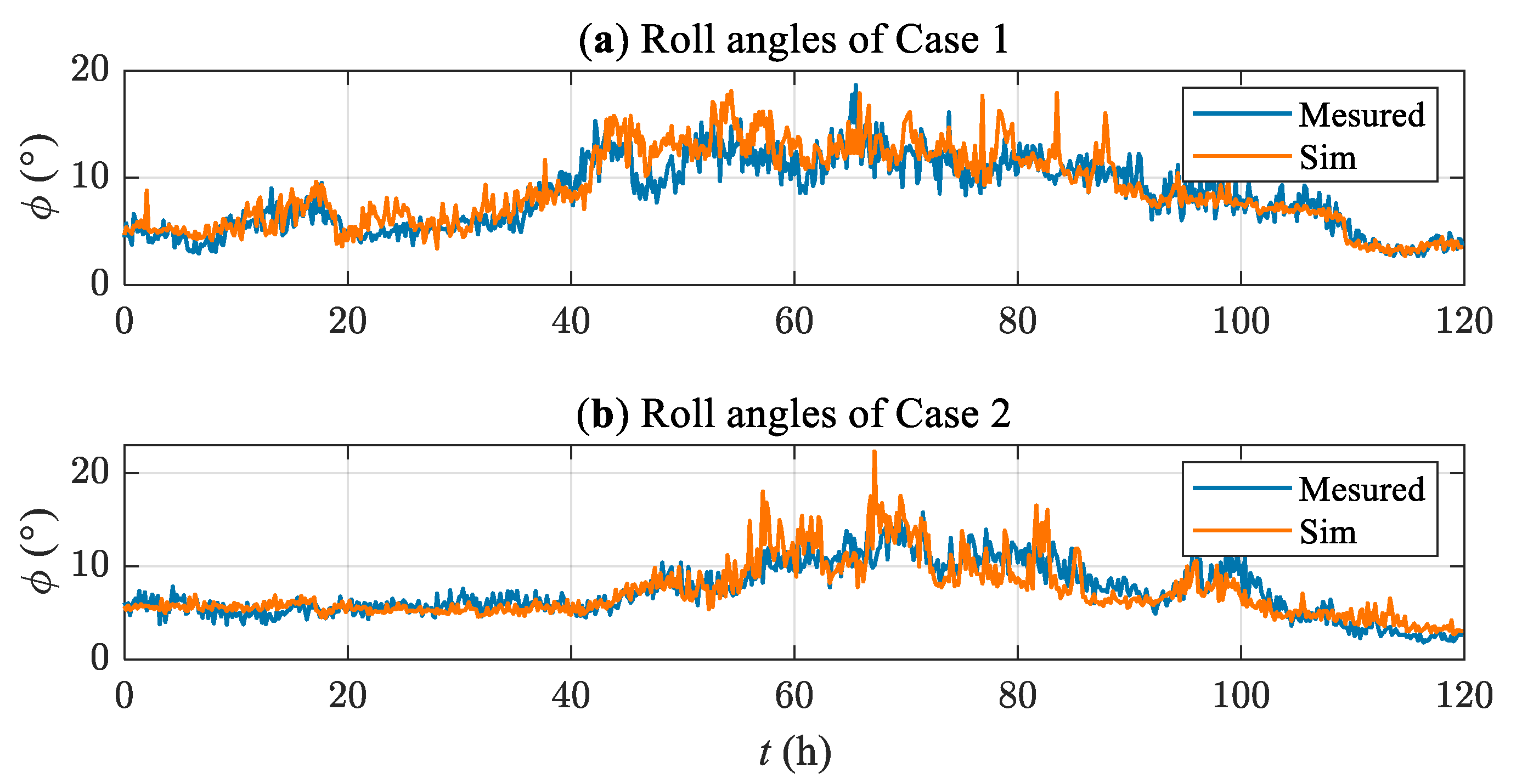
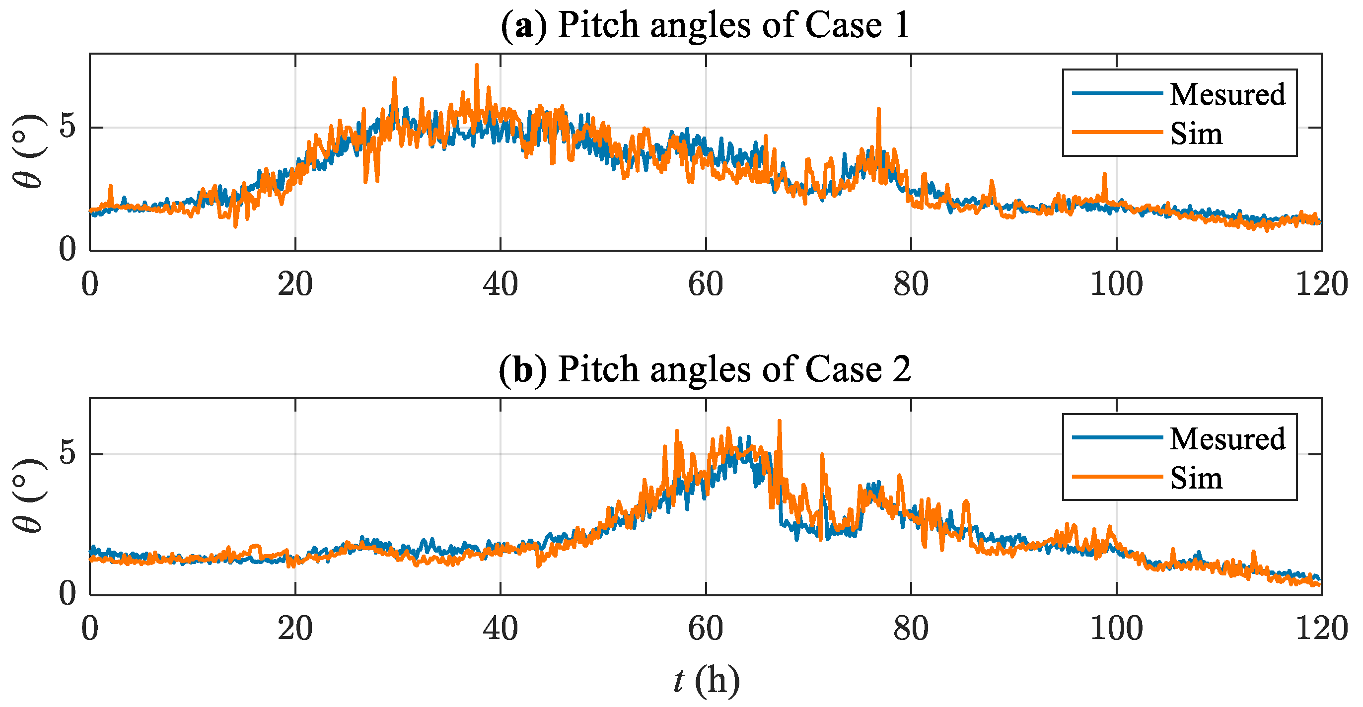
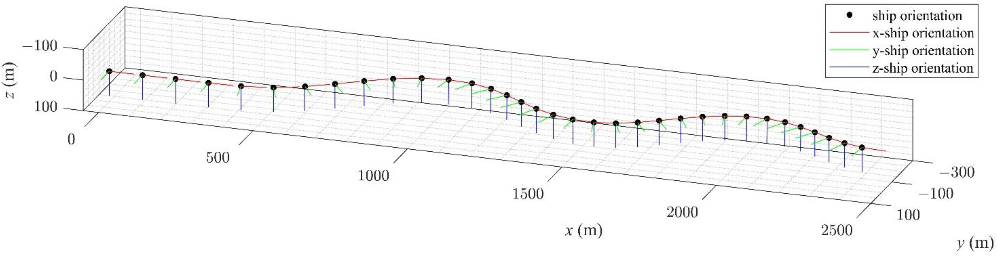
2.2. Ship Motion Simulation and Validation

Once the physical ship motion model was established, the ship motion could be simulated based on the model. There were three main input quantities used to drive the simulation, which were hydrodynamic coefficients, the control command of the rudder and propeller, and environmental vectors. The simulation flowchart is depicted in Figure 2. At the beginning of the simulation, all of the motion statuses were initialized and employed to perform the interpolations in the hydrodynamic and environment databases. In addition, the interpolation methods were provided in the mentioned work [27,30]. The hydrodynamic coefficients and environmental information were obtained through interpolations. The environmental databases could be constructed by ocean observation data or ocean hindcast data [31], which could improve the accuracy of the ship motion simulation in the actual seas [30]. Nevertheless, the environment database was optional. The wind, current, and wave vector could also be generated by a user-customized value, which provided a flexible way to simulate the ship motion under various environmental conditions.

Since the physical motion model consisted of differential equations, the motion status could be numerically iterated by the fourth-order Runge–Kutta method. In addition to the hydrodynamic coefficients and environmental information, the command of the propeller and rudder was another important input value. The command of the propeller revolution and rudder angle could be set by manual input, a group of fixed values, or real measured data from onboard sensors. Moreover, the model could be reinitialized if requested. The stop flag could either be a time period or iteration steps, and the simulation pipeline would stop if it reached the defined period or iteration steps; otherwise, the new state would be sent back to the databases to obtain the hydrodynamic coefficients and environmental information needed for the next iteration.

The linear accelerations and angular velocities were the major data measured from shipborne inertial sensors. Therefore, the purpose of the ship motion simulation was to reproduce these two kinds of data. Since the inertial sensor was fixedly connected to the ship, the accuracy of the ship motion simulation directly determined the accuracy of the inertial measurement data simulation. As discussed in the aforementioned work [26,30], the simulation of planar maneuvering motions, including the surge, sway, and yaw, were compared with the onboard measured data of a bulk carrier. The average RMSE of the one-hour simulated trajectories (surge, sway) and headings (yaw) were 0.3254 n mile and 8.15°, respectively. However, we only provided a rough validation of the simulated rolling motion. In order to adequately verify the modeling method before inertial measurement simulation, the same onboard measured data were employed [30], and the pitching and rolling motion were simulated based on the purposed simulation method. Both of the shipboard measured angles and simulated angles are given in Figure 3 and Figure 4. Furthermore, the wave encounter angles were between −2.3° and 106.8° in case one and between −3.4° and 152.7° in case two. The maximum wind speeds were 17.38 m/s for case one and 14.25 m/s for case two, corresponding to level eight (gale) and level seven (near gale) on the Beaufort scale, respectively. The maximum values of the significant wave height were 6.34 m for case one and 5.74 m for case two, respectively, corresponding to the same levels on the Beaufort scale as mentioned above. The detailed environmental conditions of the two cases were illustrated in our previous work [30].

Because the roll and pitch angles oscillated at a high frequency at all times, this paper adopted the zero up-crossing method consistent with the literature [30] to process the data to reach a better visual effect. The measured data in Figure 3 and Figure 4 represent the shipborne inertial measurement of the bulk carrier, and the simulated data were generated by our method. It can be clearly seen that the trend of the simulated value agreed with the measured value, and the amplitude was also consistent. Moreover, the RMSE of the roll angles in cases one and two were 1.31° and 1.19°, and the relative errors were 14.5% and 16.4%, respectively. The RMSE of the pitch angles in cases one and two were 0.42° and 0.31°, the relative errors were 15.2% and 16.5%, respectively. In summary, the average relative error of all simulated roll and pitch angles was about 15.7%, which indicates that the proposed method was applicable to simulate the ship’s motion state under environmental disturbances. Moreover, both the arrangement of the shipborne inertial sensors and the detailed voyage information of cases one and two were referred to the literature [30].

3. Modeling of Inertial Sensors

The error model was an essential element in the inertial measurement simulation. This section first explains the main error sources of inertial sensors and then introduces the measurement model of shipborne inertial sensors. Subsequently, according to the propagation characteristics of the random errors, stochastic error models in the time domain were established. In order to realize the simulation of inertial measurement data, the discretization process of stochastic error is derived, and the detailed content is described as follows:

3.1. Measurement Model for Inertial Sensors

An inertial sensor combined linear accelerations from an accelerometer and rotations from a gyroscope to deliver navigation parameters and position update information [32]. Both of the accelerometer and gyroscope sensors contained two main types of errors which were deterministic errors such as scale factor, bias, misalignment, and stochastic errors such as bias instability and measurement noise as shown in Figure 5. The bias of an inertial sensor was the offset of its output signal from the actual acceleration value. In addition, the misalignment error referred to an axis-to-axis error and an axis-to-package error. The former describes the alignment condition of each accelerometer and gyroscope axis compared to the ideal mutual orthogonality and the latter indicates the alignment condition in each axis related to the sensor package. Furthermore, the scale factor error was the ratio of the output error over the input and is typically expressed as a percentage. Bias instability was the random variation in the bias computed over a specified sample time and averaging time interval, which led to the angle and velocity integration error growth proportional to the time. Moreover, the measurement noise was the unwanted signal generated from internal electronics that always exists in sensors.

The complete measurement model of an inertial sensor is shown in Equation (11). Where, the subscripts “$a$” and “$g$” represent the accelerometer and gyroscope, ${\mathit{M}}_{a/g}$ is the axis-to-axis misalignment error matrices, ${\mathit{S}}_{a/g}$ is the scale error matrices, ${\mathit{b}}_{a/g}$ is the bias vectors, and ${\mathit{n}}_{a/g}$ is the measurement noise vectors. Moreover, the ${\mathit{a}}_I$ and ${\mathit{\omega }}_I$ are the initial uncorrected measurement values of acceleration and angular velocity vectors which are denoted by subscript “$I$”. The ${\mathit{a}}_C$ and ${\mathit{\omega }}_C$ are the corrected measurement value vectors which are denoted by subscript “$C$”. The detailed form of the matrices and vectors above are defined as in Equation (12).

$$\{\begin{array}{c}{\mathit{a}}_C={\mathit{M}}_a{\mathit{S}}_a\left({\mathit{a}}_I+{\mathit{b}}_a+{\mathit{n}}_a\right)\\ {\mathit{\omega }}_C={\mathit{M}}_g{\mathit{S}}_g\left({\mathit{\omega }}_I+{\mathit{b}}_g+{\mathit{n}}_g\right)\end{array}$$

(11)

$${\mathit{M}}_{a/g}=\left[\begin{array}{ccc}1& m_{xy}& m_{xz}\\ m_{yx}& 1& m_{yz}\\ m_{zx}& m_{zy}& 1\end{array}\right],{\mathit{S}}_{a/g}=\left[\begin{array}{ccc}{s}_x& 0& 0\\ 0& s_y& 0\\ 0& 0& s_z\end{array}\right],{\mathit{b}}_{a/g}=\left[\begin{array}{c}{b}_x\\ b_y\\ b_z\end{array}\right],{\mathit{n}}_{a/g}=\left[\begin{array}{c}{n}_x\\ n_y\\ n_z\end{array}\right]$$

(12)

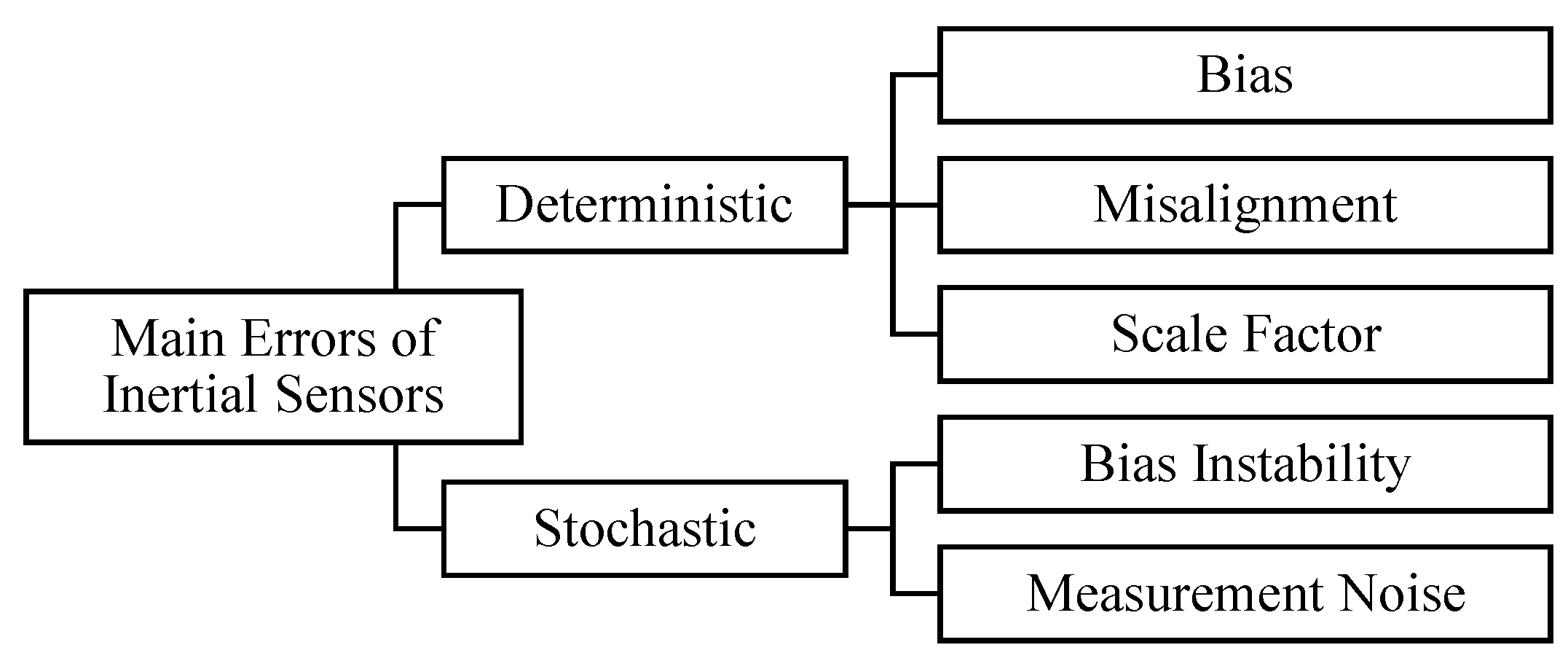
3.2. Stochastic Error Model for Inertial Sensors

The variation of stochastic errors of inertial sensors is commonly described as a random process. However, the exact values of stochastic errors were not obtainable, the noise covariance was employed to approximately describe the strength of the bias instability and measurement noise, and estimated by the widely used Allan variance analysis [33]. Based on the random process theory, the measurement noise of inertial sensors could be modeled by a Gaussian noise ${\mathit{n}}_t\left(t\right)$ with a zero-mean and covariance ${\mathit{\sigma }}_t^2$ in continuous time. The following set of equations was used to describe the measurement noise of both the accelerometer and gyroscope, where the Dirac delta function $\delta \left(t_1-t_2\right)$ indicates that the noise at each moment was independent of each other. Furthermore, the larger the value of the covariance, the stronger the noise of the inertial measurement.

$$\begin{array}{c}{\mathit{n}}_t\left(t\right)~\mathcal{N}\left(0,{\mathit{\sigma }}_t^2\right)\\ E\left[{\mathit{n}}_t\left(t_1\right){\mathit{n}}_t\left(t_2\right)\right]={\mathit{\sigma }}_t^2\delta \left(t_1-t_2\right)\\ \delta \left(t_1-t_2\right)=\{\begin{array}{c}\begin{array}{cc}1,& t_1=t_2\end{array}\\ \begin{array}{cc}0,& t_1\ne t_2\end{array}\end{array}\end{array}$$

(13)

The actual measured inertial data were discrete sampling values. As the sampling frequency of inertial sensors were generally over 100 Hz, it could be assumed that the noise remained unchanged in each sampling interval. Therefore, the discrete measurement noise model is given by:

$$\begin{array}{c}{\mathit{n}}_d\left[k\right]~\mathcal{N}\left(0,{\mathit{\sigma }}_d^2\right)\\ {\mathit{n}}_d\left[k\right]={\mathit{n}}_t\left(t_0+\Delta t\right)\approx \frac{1}{\Delta t}{{\displaystyle \int }}_{t_0}^{t_0+\Delta t}{\mathit{n}}_t\left(\tau \right)\mathrm{d}\tau \end{array}$$

(14)

Here, ${\mathit{n}}_d\left[k\right]$ denotes the discrete measurement noise at the kth moment, the discrete noise covariance is represented by ${\mathit{\sigma }}_d^2$, and $\Delta t$ is the sampling interval. Based on Equations (13) and (14), the relation between continuous and discrete measurement noise is derived by:

$$\begin{gathered} {\mathit{\sigma }}_d^2=E[{\left({\mathit{n}}_d\left[k\right]\right)}^2]=\frac{1}{\Delta t^2}{{\displaystyle \int }}_{t_0}^{t_0+\Delta t}{{\displaystyle \int }}_{t_0}^{t_0+\Delta t}E\left[{\mathit{n}}_t\left(t\right){\mathit{n}}_t\left(\tau \right)\right]\mathrm{d}t\mathrm{d}\tau \\ =\frac{1}{\Delta t^2}{{\displaystyle \int }}_{t_0}^{t_0+\Delta t}{{\displaystyle \int }}_{t_0}^{t_0+\Delta t}{\mathit{\sigma }}_t^2\delta \left(t-\tau \right)\mathrm{d}t\mathrm{d}\tau \\ =\frac{{\mathit{\sigma }}_t^2}{\Delta t^2}{{\displaystyle \int }}_{t_0}^{t_0+\Delta t}1\mathrm{d}\tau =\frac{{\mathit{\sigma }}_t^2}{\Delta t} \end{gathered}$$

(15)

In addition to being affected by the measurement noise, the bias of the inertial sensors also changed continuously over time. Generally, the Wiener process is used to describe the variation of bias [34]. The following set of equations were used to explain the bias instability of both the accelerometer and gyroscope:

$$\begin{array}{c}w\left(t\right)~\mathcal{N}\left(0,1\right)\\ \dot{\mathit{b}}\left(t\right)={\mathit{n}}_{bt}\left(t\right)={\mathit{\sigma }}_{bt}w\left(t\right)\\ \mathit{b}\left(t_0+\Delta t\right)=\mathit{b}\left(t_0\right)+{{\displaystyle \int }}_{t_0}^{t_0+\Delta t}{\mathit{n}}_{bt}\left(t\right)\mathrm{d}t\end{array}$$

(16)

where $w\left(t\right)$ is the Gaussian white noise with a variance of 1. The function ${\mathit{n}}_{bt}\left(t\right)$ represents the derivative of the bias in continuous time and the ${\mathit{\sigma }}_{bt}$ is the standard deviation which indicates the strength of bias variation.

Similarly, the bias of inertial sensors could be assumed unchanged in each sampling interval due to a high sampling frequency. The discrete form of the variation of the bias is given:

$$\begin{array}{c}w\left[k\right]~\mathcal{N}\left(0,1\right)\\ {\mathit{b}}_d\left[k\right]={\mathit{b}}_d\left[k-1\right]+{\mathit{\sigma }}_{bd}w\left[k\right]\end{array}$$

(17)

where ${\mathit{b}}_d\left[k\right]$ is the discrete bias at the kth moment and ${\mathit{\sigma }}_{bd}$ denotes the discrete standard deviation related to ${\mathit{\sigma }}_{bt}$. The relation between continuous and discrete bias can be derived based on Equations (16) and (17):

$$\begin{array}{c}E\left[{\mathit{b}}^2\left(t_0+\Delta t\right)\right]=E\left[{\mathit{b}}^2\left(t_0\right)+{{\displaystyle \int }}_{t_0}^{t_0+\Delta t}{{\displaystyle \int }}_{t_0}^{t_0+\Delta t}{\mathit{\sigma }}_{bt}^2\delta \left(t-\tau \right)\mathrm{d}t\mathrm{d}\tau \right]\\ =E\left[{\mathit{b}}^2\left(t_0\right)\right]+{\mathit{\sigma }}_{bt}^2\Delta t\\ \Rightarrow {\mathit{\sigma }}_{bd}^2={\mathit{\sigma }}_{bt}^2\Delta t\end{array}$$

(18)

Finally, the derivation from continuous to discrete measurement noise and bias are clearly given by Equations (15) and (18), which established one of the foundations of the inertial measurement data simulation. Once we were able to simulate the acceleration and angular velocity of the vehicle without error interference, then, with the above equations, we could artificially add the error terms at any sampling frequency to the ideal inertial measurement data to simulate realistic inertial sensors.

4. Simulation Framework of Shipborne Inertial Sensors

In this section, the idea of using the ship motion model and sensor error model to simulate shipborne inertial sensors is explained firstly. Then, the implementation details of three ROS nodes are illustrated and the complete simulation framework is developed. Finally, the simulation results of the shipborne inertial measurement are provided.

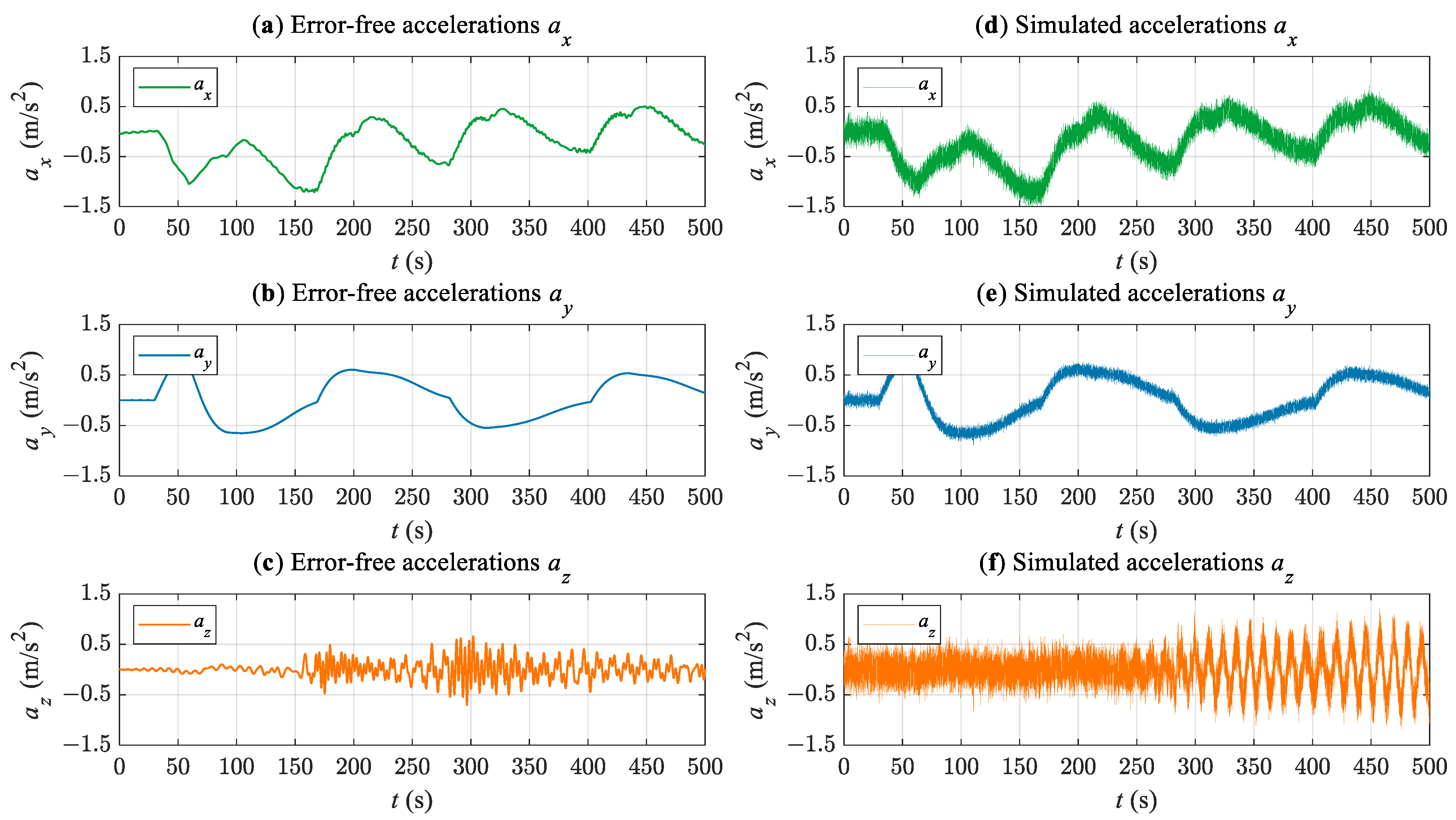
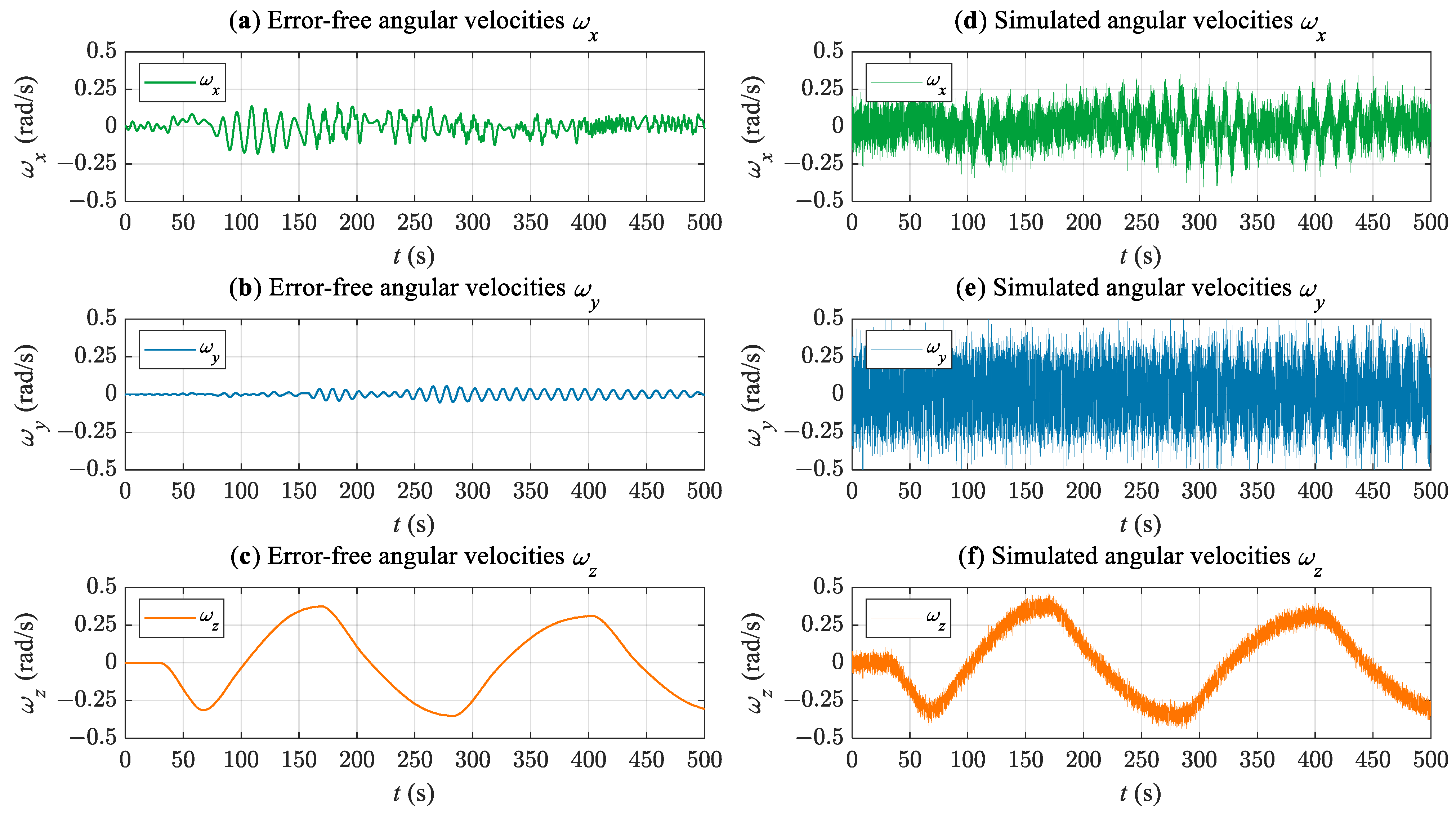
4.1. Shipborne Inertial Sensors Simulation

The method of the shipborne inertial sensors simulation was composed of two basic steps. First of all, the ideal inertial measurement data without any error were simulated based on the physical motion model of ships proposed in Section 2. Subsequently, the artificial deterministic and stochastic errors were generated at any specified sampling frequency based on the discrete error models derived in Section 3.

The relations between simulated inertial measurement data and the simulated ship motion status are described by the following set of equations:

$${\mathit{a}}_M={\left[a_x,a_y,a_z\right]}^{\mathrm{T}}={\left[\dot{u},\dot{v},\dot{w}\right]}^{\mathrm{T}},{\mathit{\omega }}_M={\left[{\omega }_x,{\omega }_y,{\omega }_z\right]}^{\mathrm{T}}={\left[p,q,r\right]}^{\mathrm{T}}$$

(19)

$$\{\begin{array}{c}{\mathit{a}}_S\left[k\right]={\mathit{M}}_a^{-1}{\mathit{S}}_a^{-1}{\mathit{a}}_M\left[k\right]-{\mathit{b}}_a\left[k\right]-{\mathit{n}}_a\left[k\right]\\ {\mathit{n}}_a\left[k\right]~\mathcal{N}\left(0,\frac{{\mathit{\sigma }}_{a,t}^2}{\Delta t}\right)\\ {\mathit{b}}_a\left[k\right]={\mathit{b}}_a\left[k-1\right]+{\mathit{\sigma }}_{ba,t}\sqrt{\Delta t}·w\left[k\right]\end{array}$$

(20)

$$\{\begin{array}{c}{\mathit{\omega }}_S\left[k\right]={\mathit{M}}_g^{-1}{\mathit{S}}_g^{-1}{\mathit{\omega }}_M\left[k\right]-{\mathit{b}}_g\left[k\right]-{\mathit{n}}_g\left[k\right]\\ {\mathit{n}}_g\left[k\right]~\mathcal{N}\left(0,\frac{{\mathit{\sigma }}_{g,t}^2}{\Delta t}\right)\\ {\mathit{b}}_g\left[k\right]={\mathit{b}}_g\left[k-1\right]+{\mathit{\sigma }}_{bg,t}\sqrt{\Delta t}·w\left[k\right]\end{array}$$

(21)

where ${\mathit{a}}_M$ and ${\mathit{\omega }}_M$ are vectors of linear acceleration and angular velocity that were generated by the ship motion model. These two vectors could be regarded as ideal inertial measurements. Correspondingly, ${\mathit{a}}_S$ and ${\mathit{\omega }}_S$ are vectors of simulated linear acceleration and angular velocity which were produced by adding artificial errors to ${\mathit{a}}_M$ and ${\mathit{\omega }}_M$. The covariance terms ${\mathit{\sigma }}_{a,t}^2$ and ${\mathit{\sigma }}_{g,t}^2$ denote the strength of the measurement noise of the accelerometer and gyroscope. Likewise, ${\mathit{\sigma }}_{ba,t}$ and ${\mathit{\sigma }}_{bg,t}$ represent the strength of bias instability of the above sensors. The functional relationships between continuous and discrete covariance were derived in Equations (15) and (18), and directly employed in Equations (20) and (21).

It should be noted that in addition to the influence of errors, the installation position of the sensor was also a very important factor. As defined in Figure 1, the origin of the ship motion model was chosen to coincide with the midship point. That is, all the simulated motion statuses were defined relative to the origin. Since the ultimate goal of the inertial sensor simulation was to develop and test the sensor fusion algorithms. A practical approach is to treat the simulation tests and actual tests separately. At the stage of the simulation test, the installation position of inertial sensors could be assumed to exactly coincide with the defined origin, for which there was no need to calibrate, and the developers could focus on the fusion algorithms. Moreover, at the stage of the actual ship test, the installation position of the actual sensors would be calibrated. All of the spatial transformation matrices were conveniently managed by the ROS transform trees, and the developers could be confident that the data were in the coordinate frame that they wanted without requiring the knowledge of all the coordinate frames in the system [35].

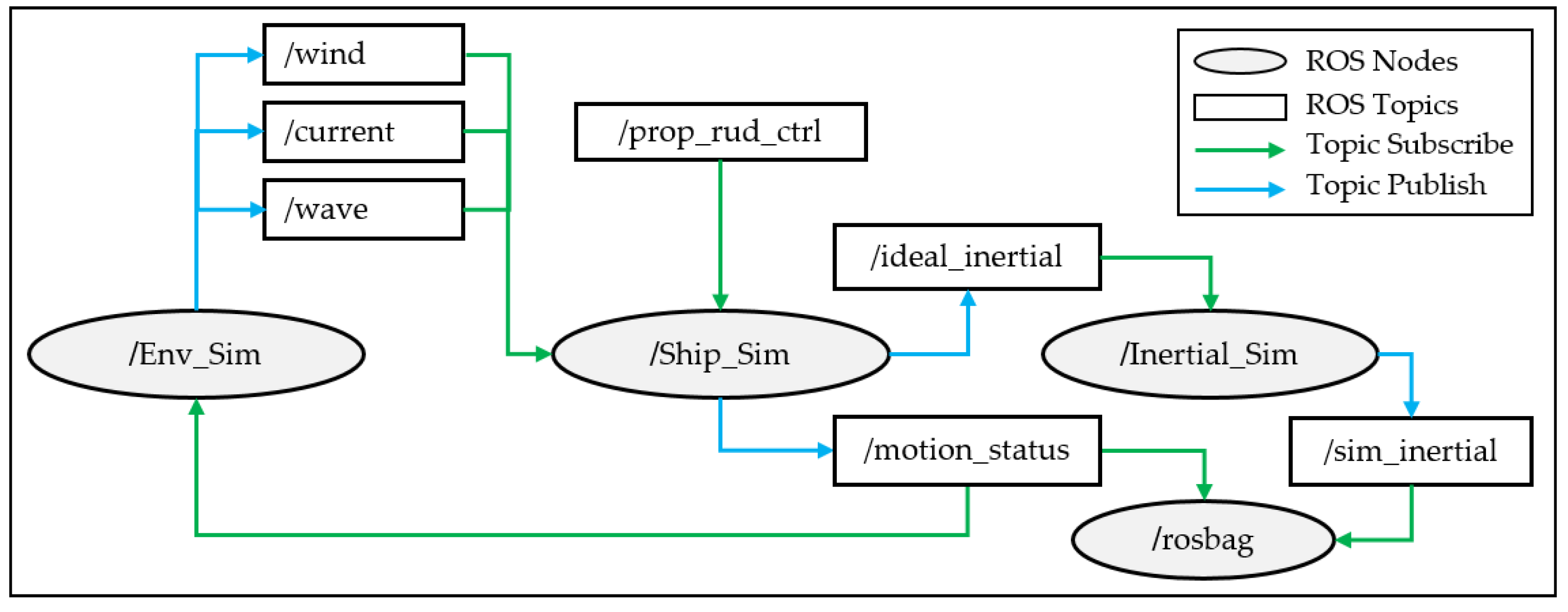
4.2. Universal Simulation Framework Based on the ROS

The ROS is an open-source robot middleware and a collection of software frameworks for robot development which had been developed based on a graph architecture [36]. The programs in the ROS can publish and receive various information as nodes in the computation graph, such as sensor data, control signals, state information, planning commands, etc. We developed a simulation framework based on the ROS, and the structure is shown in Figure 6.

There were three main nodes implemented in the computation graph, which were “Env_Sim”, “Ship_Sim”, and “Inertial_Sim”. The “Env_Sim” node subscribes to the motion status topic published from the “Ship_Sim” node, and publishes the specified environmental information. As we discussed in Section 2.2, the motion state was employed to perform the interpolations in the environment databases. The “/wind” and “/current” topics use the “geometry_msgs/Vector3Stamped” message type which includes a three-dimensional vector to store the speed and direction of the wind/current and a timestamp. Similarly, the “geometry_msgs/Vector3Stamped” message type is also used for the “/wave” topic to store the timestamp, direction, height, and period of a wave vector.

The “Ship_Sim” node subscribes to two kinds of topics which are the environmental vectors and the “prop_rud_ctrl”, and publishes two kinds of topics which are the ship motion status and ideal inertial data. The “geometry_msgs/Vector3Stamped” message type is adopted to store the command of propeller revolutions and rudder angles in the topic “prop_rud_ctrl”. The “nav_msgs/Odometry” message type is employed to store the linear and angular velocities, position, orientation, and timestamp of the ship. In addition, the message type “sensor_msgs/Imu” consists of acceleration and angular velocity vectors used for both the ideal inertial measurement data topic “ideal_inertial” and simulated inertial measurement data topic “sim_inertial”.

The “Inertial_Sim” node subscribes to the “ideal_inertial” topic and adds artificial errors according to Equations (20) and (21). All of the necessary random numbers are generated based on the C++ 11 random number engines. Furthermore, the simulated acceleration and angular velocity vectors are published by this node. Finally, the “rosbag” node from the ROS is applied to serialize and store the ship motion status and simulate the inertial measurement data, which makes the data be easily verified and reused.

To summarize, any nodes used for fusion perception could obtain the inertial measurement data with errors by subscribing to topic “sim_inertial”, and the poses of the ship in the virtual three-dimensional scene could be driven by an error-free data topic “motion_status”. Moreover, if there were no environment databases available, the user could manually publish the “/wind”, “/current”, and “/wave” topics. Since all of the messages used in the framework came from native message types of ROS, it was also very convenient to develop a user-defined environmental message publishing node. Accordingly, the “Ship_Sim” is also a replaceable node if users could provide the ideal inertial measurement data by same message type by themselves.

4.3. Simulation Results

Simulation results of the shipborne inertial sensor are provided in this section. The artificial standard deviation of the continuous measurement noise and bias instability adopted in the simulations are shown in

Table 2. Settings of artificial measurement noise and bias instability.

Error Type	Accelerometer	Gyroscope
Measurement Noise	0.013 m/s2	0.0084 rad/s
Bias Instability	0.00063 m/s2	0.000087 rad/s

. The settings of these parameters refer to the open-source inertial sensor calibration toolkit [37]. Since the deterministic error was only a fixed offset or scaling of the original data, we focused on the simulation of stochastic errors. The axis-to-axis misalignment error matrices ${\mathit{M}}_{a/g}$ and scale error matrices ${\mathit{S}}_{a/g}$ were set as the identity matrices. Moreover, the initial bias vectors ${\mathit{b}}_{a/g}$ were set as the zero vectors. The covariance ${\mathit{\sigma }}_{a/g,t}$ and ${\mathit{\sigma }}_{ba/bg,t}$ in Equations (20) and (21) were matrix values; here we assumed these matrices were diagonal and of the same order of magnitude for all axes in practice. Although this hypothesis was adopted in our simulations, developers could still customize any covariance matrix according to the characteristics of their target sensors.

The above-mentioned simulation framework and error parameters were employed to simulate the shipborne inertial sensors. The same bulk carrier [30] and hydrodynamic coefficients database [27] were adopted in the simulations. The sampling frequency of the shipborne inertial sensor was set to 100 Hz ($\Delta t$ = 0.01 s).

The simulation settings were arranged as follows: the ship sailed with a heading of 0° at the initial moment, the propeller revolution was fixed at 122 r/m, and a 10°/10° zigzag maneuver was carried out when the ship motion reached a steady status, and the simulation duration was set to 500 s. The main reason for choosing the zigzag test was that the test would fully excite the ship motion and make the motion state change periodically, so that the inertial simulation results were easier to observe. Moreover, the average direction of the wind in the simulated environment was 0°, and the average wind speed was 2 m/s; the average direction of the ocean current was 0°, and the average current velocity was 0.1 m/s; the main wave direction was 0°, and the significant wave height was 1.0 m; the average wave period was 8.0 s.

The “rosbag” node was used to record the error-free ship motion status and simulated inertial measurement data. The recorded ship position and orientation are depicted in Figure 7. The poses of the ship were interpreted from the “motion_status” topic and displayed by the body-fixed frames. Since the data published by the nodes were 100 Hz, in order to ensure clarity, the original poses were sparsely processed.

The ideal and the simulated inertial measurement data were recorded by the same method. The error-free accelerations generated by the ship motion model and the simulated accelerations with artificial errors are provided in Figure 8. Correspondingly, the angular velocities are provided in Figure 9.

The first point to note is that the accelerations and angular velocities from the physical ship motion model were very smooth and without the interference of measurement noise and bias instability. Since the position was obtained by acceleration integration, the changing trend of the acceleration components $a_x$ and $a_y$ in Figure 8 was completely consistent with the x and y coordinates of the track points in Figure 7. Similarly, the orientations were integrated by angular velocities; therefore, the varying of the yaw angle rate ${\omega }_z$ also agreed with the ship orientations shown in Figure 7. As can be seen from the right parts of Figure 8 and Figure 9, the inertial measurement data became more realistic after adding the artificial measurement noise and bias instability. Further, the data in Figure 8 were partially intercepted and enlarged to illustrate the difference between the noise and high-frequency components in the simulated results. As mentioned in the ship motion model, the ship was disturbed by environmental effects, especially the waves. The first-order wave forces and moments contributed to the high-frequency components of the simulated ship motion as shown in the left part of Figure 10. However, these high-frequency components could not completely reflect the characteristics of the shipborne inertial sensors compared with the artificial noise in the right part of Figure 10. It follows that model-based ship motion simulation could not be directly used as the simulation result of shipborne inertial sensors.

As mentioned in Section 2, the simulation method of ship motions was validated by shipboard measurement data. Therefore, we could consider that the simulation of the ideal motion state was accurate. The differences between the ideal motion state and the actual inertial measurement data mainly consisted of errors and noise. Therefore, the process from the ideal motion state to the realistic inertial measurement was to add artificial errors. As can be seen from Figure 8 to Figure 9, the errors oscillate around the ideal values due to the zero-mean setting of the Gaussian distribution in Equations (20) and (21). Consequently, the above results indicated that the proposed framework is rational and applicable for simulations of shipborne inertial sensors.

5. Discussion

A universal simulation framework was implemented based on the ROS and ship motion model in this paper. The proposed framework could perform a realistic simulation of shipborne inertial sensors. Moreover, the modeling and simulation method in this paper also gave insight for building a perfect virtual test environment for developing and testing shipboard multi-sensor fusion perception algorithms. However, there were certain assumptions in the proposed method. The limitations are discussed here which provide directions for future studies. Firstly, only the measurement noise and random walks of bias were considered in the simulations. However, there were more than two stochastic error sources in real inertial sensors, such as temperature error and high-frequency vibration noise from the ship engines. Secondly, the errors discussed in this paper all conformed to the Gaussian distribution which was a practical solution in most literature [3,13], whereas it may be impractical and inaccurate to use the Gaussian distribution to describe real sensor errors. Given the above limitations, it is necessary to further study other error sources and simulation mechanisms of shipborne inertial sensors to reach a physically accurate simulation. Moreover, direct comparisons between the simulated inertial measurement data and the real sensors under the same maneuvers and environmental conditions based on a complete sensor error model should be conducted in future work.

6. Conclusions

In this paper, the physical-based ship motion model was integrated with the Robot Operating System to simulate the shipborne inertial sensors. The proposed ship motion model could reflect the physical movement characteristics of ship maneuvering under realistic environmental disturbances based on well-modeled differential equations. The accuracy and applicability of the model were further verified by the comparison with actual ship measurement data. However, the acceleration and angular velocity data generated by ship motion simulation contained no error and noise items, which brought up a gap between the realistic inertial measurement data. Through an in-depth analysis of the error mechanism of inertial sensors, the discretization process of continuous measurement noise and bias instability was derived. Based on the above derivation conclusions, artificial errors could be easily added to the ideal accelerations and angular velocities, which would close the gap between the simulated sensors and real sensors. Moreover, the inertial simulation data could be generated at any customized sampling frequency thanks to the discretized stochastic error model. Finally, a universal simulation framework was implemented and the features of this framework were summarized as follows:

• The physical-based ship motion model was established which could provide a realistic simulation of the ship motion status under environmental disturbances;
• The framework was designed by a module decoupling idea. The interaction between modules only relied on unified data interfaces and the modules were replaceable;
• The native ROS message types were employed in the framework which could directly interact with algorithms designed for real sensors;
• The error terms, error strength, sampling frequency, environmental information input, and rudder and propeller control input were all customizable which made the framework more flexible to handle different environmental conditions and sensor settings.

The benefit from the aforementioned features, the proposed framework could perform a realistic simulation of shipborne inertial sensors which built a research foundation for the fusion perception algorithm based on visual–inertial and laser–inertial sensors in the research field of ASVs. The current work built a connection between the ship motion model and the shipborne inertial sensor simulation. However, it was a preliminary exploration in the field of the shipborne sensor simulation. In the near future, not only will the complete sensor models be developed, but sufficient experiments on real ASVs will be performed to further promote our work.

References

1. Karetnikov, V.; Ol’khovik, E.; Butsanets, A.; Ivanova, A. Development of Methods for Maneuvering Trials of Autonomous Ships in Test Water Area. In Proceedings of the XIII International Scientific Conference on Architecture and Construction 2020, Singapore, 22–24 September 2020; pp. 40–46. [Google Scholar] [CrossRef]
2. Huang, W.; Wang, K.; Lv, Y.; Zhu, F. Autonomous Vehicles Testing Methods Review. In Proceedings of the 2016 IEEE 19th International Conference on Intelligent Transportation Systems (ITSC), Rio de Janeiro, Brazil, 1–4 November 2016; pp. 163–168. [Google Scholar] [CrossRef]
3. Shah, S.; Dey, D.; Lovett, C.; Kapoor, A. AirSim: High-Fidelity Visual and Physical Simulation for Autonomous Vehicles. In Field and Service Robotics; Springer Proceedings in Advanced Robotics; Hutter, M., Siegwart, R., Eds.; Springer International Publishing: Cham, Switzerland, 2018; pp. 621–635. [Google Scholar] [CrossRef] [Green Version]
4. Thombre, S.; Zhao, Z.; Ramm-Schmidt, H.; García, J.M.V.; Malkamäki, T.; Nikolskiy, S.; Hammarberg, T.; Nuortie, H.; Bhuiyan, M.Z.H.; Särkkä, S.; et al. Sensors and AI Techniques for Situational Awareness in Autonomous Ships: A Review. IEEE Trans. Intell. Transp. Syst. 2020, 1–20. [Google Scholar] [CrossRef]
5. Wright, R.G. Intelligent Autonomous Ship Navigation Using Multi-Sensor Modalities. TransNav Int. J. Mar. Navig. Saf. Sea Transp. 2019, 13, 503–510. [Google Scholar] [CrossRef]
6. Han, J.; Cho, Y.; Kim, J.; Kim, J.; Son, N.; Kim, S.Y. Autonomous Collision Detection and Avoidance for ARAGON USV: Development and Field Tests. J. Field Robot. 2020, 37, 987–1002. [Google Scholar] [CrossRef]
7. Liu, W.; Liu, Y.; Bucknall, R. A Robust Localization Method for Unmanned Surface Vehicle (USV) Navigation Using Fuzzy Adaptive Kalman Filtering. IEEE Access 2019, 7, 46071–46083. [Google Scholar] [CrossRef]
8. Qin, T.; Li, P.; Shen, S. VINS-Mono: A Robust and Versatile Monocular Visual-Inertial State Estim ator. IEEE Trans. Robot. 2018, 34, 1004–1020. [Google Scholar] [CrossRef] [Green Version]
9. Qin, C.; Ye, H.; Pranata, C.E.; Han, J.; Zhang, S.; Liu, M. LINS: A Lidar-Inertial State Estimator for Robust and Efficient Navigation. In Proceedings of the 2020 IEEE International Conference on Robotics and Automation (ICRA), Virtual Conference, 31 May–31 August 2020; pp. 8899–8906. [Google Scholar] [CrossRef]
10. Mur-Artal, R.; Montiel, J.M.M.; Tardós, J.D. ORB-SLAM: A Versatile and Accurate Monocular SLAM System. IEEE Trans. Robot. 2015, 31, 1147–1163. [Google Scholar] [CrossRef] [Green Version]
11. Zhang, J.; Singh, S. LOAM: Lidar Odometry and Mapping in Real-Time. In Proceedings of the Robotics: Science and Systems Conference (RSS), Berkeley, CA, USA, 14–16 July 2014; pp. 109–111. [Google Scholar] [CrossRef]
12. Rosique, F.; Navarro, P.J.; Fernández, C.; Padilla, A. A Systematic Review of Perception System and Simulators for Autonomous Vehicles Research. Sensors 2019, 19, 648. [Google Scholar] [CrossRef] [PubMed] [Green Version]
13. Koenig, N.; Howard, A. Design and Use Paradigms for Gazebo, an Open-Source Multi-Robot Simulator. In Proceedings of the IEEE/RSJ International Conference on Intelligent Robots and Systems (IROS), Sendai, Japan, 28 September–2 October 2004; Volume 3, pp. 2149–2154. [Google Scholar] [CrossRef] [Green Version]
14. Rivera, Z.B.; De Simone, M.C.; Guida, D. Unmanned Ground Vehicle Modelling in Gazebo/ROS-Based Environments. Machines 2019, 7, 42. [Google Scholar] [CrossRef] [Green Version]
15. Bernardeschi, C.; Fagiolini, A.; Palmieri, M.; Scrima, G.; Sofia, F. ROS/Gazebo Based Simulation of Co-Operative UAVs. In Modelling and Simulation for Autonomous Systems; Mazal, J., Ed.; Lecture Notes in Computer Science; Springer International Publishing: Cham, Switzerland, 2019; pp. 321–334. [Google Scholar] [CrossRef]
16. Garzón, M.; Spalanzani, A. A Hybrid Simulation Tool for Autonomous Cars in Very High Traffic Scenarios. In Proceedings of the 2018 15th International Conference on Control, Automation, Robotics and Vision (ICARCV), Singapore, 18–21 November 2018; pp. 803–808. [Google Scholar] [CrossRef] [Green Version]
17. Bingham, B.; Aguero, C.; McCarrin, M.; Klamo, J.; Malia, J.; Allen, K.; Lum, T.; Rawson, M.; Waqar, R. Toward Maritime Robotic Simulation in Gazebo. In Oceans 2019 MTS/IEEE Seattle; IEEE: Seattle, WA, USA, 2019; pp. 1–10. [Google Scholar] [CrossRef]
18. Paravisi, M.; Santos, D.H.; Jorge, V.; Heck, G.; Gonçalves, L.M.; Amory, A. Unmanned Surface Vehicle Simulator with Realistic Environmental Disturbances. Sensors 2019, 19, 1068. [Google Scholar] [CrossRef] [PubMed] [Green Version]
19. Rong, G.; Shin, B.H.; Tabatabaee, H.; Lu, Q.; Lemke, S.; Možeiko, M.; Boise, E.; Uhm, G.; Gerow, M.; Mehta, S.; et al. LGSVL Simulator: A High Fidelity Simulator for Autonomous Driving. In Proceedings of the 2020 IEEE 23rd International Conference on Intelligent Transportation Systems (ITSC), Virtual Conference, 20–23 September 2020; pp. 1–6. [Google Scholar]
20. Autoware, AI. Available online: https://github.com/Autoware-AI/autoware.ai (accessed on 1 August 2021).
21. ApolloAuto. Available online: https://github.com/ApolloAuto/apollo (accessed on 1 August 2021).
22. Dosovitskiy, A.; Ros, G.; Codevilla, F.; Lopez, A.; Koltun, V. CARLA: An Open Urban Driving Simulator. In Proceedings of the 1st Annual Conference on Robot Learning (CoRL), Mountain View, CA, USA, 13–15 November 2017; pp. 1–16. [Google Scholar]
23. NVIDIA DRIVE Sim. Available online: https://developer.nvidia.com/drive/drive-sim (accessed on 1 August 2021).
24. Wang, Y.; Bulger, C.; Thanyamanta, W.; Bose, N. A Backseat Control Architecture for a Slocum Glider. J. Mar. Sci. Eng. 2021, 9, 532. [Google Scholar] [CrossRef]
25. Fossen, T.I. Handbook of Marine Craft Hydrodynamics and Motion Control; John Wiley & Sons, Ltd.: Chichester, UK, 2011. [Google Scholar] [CrossRef]
26. Jing, Q.; Shen, H.; Yin, Y. Motion Modeling and Simulation of Maritime Autonomous Surface Ships in Realistic Environmental Disturbances. In Proceedings of the 2020 IEEE 23rd International Conference on Intelligent Transportation Systems (ITSC), Virtual Conference, 20–23 September 2020; pp. 1–7. [Google Scholar] [CrossRef]
27. Jing, Q.; Shen, H.; Yin, Y. A Stereolithographic Model-Based Dense Body Plan Generation Method to Construct a Ship Hydrodynamic Coefficients Database. J. Mar. Sci. Eng. 2020, 8, 222. [Google Scholar] [CrossRef] [Green Version]
28. Yasukawa, H.; Yoshimura, Y. Introduction of MMG Standard Method for Ship Maneuvering Predictions. J. Mar. Sci. Technol. 2015, 20, 37–52. [Google Scholar] [CrossRef] [Green Version]
29. Liu, J.; Hekkenberg, R.; Quadvlieg, F.; Hopman, H.; Zhao, B. An Integrated Empirical Manoeuvring Model for Inland Vessels. Ocean Eng. 2017, 137, 287–308. [Google Scholar] [CrossRef]
30. Jing, Q.; Sasa, K.; Chen, C.; Yin, Y.; Yasukawa, H.; Terada, D. Analysis of Ship Maneuvering Difficulties under Severe Weather Based on Onboard Measurements and Realistic Simulation of Ocean Environment. Ocean Eng. 2021, 221, 108524. [Google Scholar] [CrossRef]
31. Chen, C.; Sasa, K.; Prpić-Oršić, J.; Mizojiri, T. Statistical Analysis of Waves’ Effects on Ship Navigation Using High-Resolution Numerical Wave Simulation and Shipboard Measurements. Ocean Eng. 2021, 229, 108757. [Google Scholar] [CrossRef]
32. Unsal, D.; Demirbas, K. Estimation of Deterministic and Stochastic IMU Error Parameters. In Proceedings of the 2012 IEEE/ION Position Location and Navigation Symposium (PLANS), Myrtle Beach, SC, USA, 23–26 April 2012; pp. 862–868. [Google Scholar]
33. El-Sheimy, N.; Hou, H.; Niu, X. Analysis and Modeling of Inertial Sensors Using Allan Variance. IEEE Trans. Instrum. Meas. 2007, 57, 140–149. [Google Scholar] [CrossRef]
34. Caron, F.; Duflos, E.; Pomorski, D.; Vanheeghe, P. GPS/IMU Data Fusion Using Multisensor Kalman Filtering: Introduction of Contextual Aspects. Inf. Fusion 2006, 7, 221–230. [Google Scholar] [CrossRef]
35. Foote, T. Tf: The Transform Library. In Proceedings of the 2013 IEEE Conference on Technologies for Practical Robot Applications (TePRA), Wpburm, MA, USA, 22–23 April 2013; pp. 1–6. [Google Scholar] [CrossRef]
36. Quigley, M.; Conley, K.; Gerkey, B.; Faust, J.; Foote, T.; Leibs, J.; Wheeler, R.; Ng, A.Y. ROS: An Open-Source Robot Operating System. In Proceedings of the ICRA Workshop on Open Source Software, Kobe, Japan, 12–17 May 2009; Volume 3, p. 5. [Google Scholar]
37. imu_utils: A ROS Package Tool to Analyze the IMU Performance. Available online: https://github.com/gaowenliang/imu_utils (accessed on 1 August 2021).
Figure 1. Coordinate systems.
Jmse 09 00900 g001
Figure 2. Flowchart of ship motion simulation.
Jmse 09 00900 g002
Figure 3. Validation of simulated rolling motion. (a) simulated roll angles of case 1; (b) simulated roll angles of case 2.
Jmse 09 00900 g003
Figure 4. Validation of simulated pitching motion. (a) simulated pitch angles of case 1; (b) simulated pitch angles of case 2.
Jmse 09 00900 g004
Figure 5. Main errors of inertial sensors.
Jmse 09 00900 g005
Figure 6. Simulation framework of shipborne inertial sensors.
Jmse 09 00900 g006
Figure 7. Time series of simulated ship poses.
Jmse 09 00900 g007
Figure 8. Error-free and simulated accelerations. (a) error-free accelerations of x direction; (b) error-free accelerations of y direction; (c) error-free accelerations of z direction; (d) simulated accelerations of x direction; (e) simulated accelerations of y direction; (f) simulated accelerations of z direction.
Jmse 09 00900 g008
Figure 9. Error-free and simulated angular velocities. (a) error-free angular velocities of x direction; (b) error-free angular velocities of y direction; (c) error-free angular velocities of z direction; (d) simulated angular velocities of x direction; (e) simulated angular velocities of y direction; (f) simulated angular velocities of z direction.
Jmse 09 00900 g009
Figure 10. Noise and high-frequency components in simulation. (a) error-free accelerations; (b) simulated accelerations.
Jmse 09 00900 g010