Hydrodynamic Climate of Port Phillip Bay

Abstract

This study is dedicated to the hydrodynamic climate of Port Phillip Bay (PPB)—a largest coastal lagoon system in Victoria, Australia. Novelty of the present study includes long-term hydrodynamic hindcast simulations integrated with a spectral wave model. Specifically, a coupled unstructured grid wave–current modelling system (SCHISM + WWM) was built upon a high resolution and advanced wave physics (ST6). This coupling system was thoroughly calibrated and validated against field observations prior to applying for 27-year hindcast and case scenarios. Data from these simulations were then used to investigate the hydrodynamic climate of PPB focusing on three main aspects: water levels, waves and currents. For sea levels, this study shows that tidal and extreme sea levels (storm tides) across a large part of PPB have a similar magnitude. The highest storm tide level is found along eastern coasts of the bay in line with the wind pattern. In the vicinity of the entrance, the extreme sea level slightly reduced, in line with wave decay due to coupling effects. This extreme level is lower than results reported by previous studies, which were not built on a wave–current coupled system. For the wave field, the mean wave direction inside PPB is strongly affected by seasonality, in line with wind patterns. The 100-year return significant wave height is above 2 m along the eastern coasts. At PPH, waves get refracted after passing the narrow entrance. For currents, this study shows that both mean variations and high percentile currents are not affected by seasonality. This highlights the fact that tidal currents dominate flow movements in PPB. However, in extreme conditions, the circulation in PPB is also driven by wind patterns, forming two gyre systems. Based on case scenarios simulations, the strongest magnitude of wind-driven currents is above 0.5 m/s and found in the confined shallow region in the southern portion of PPB.

1. Introduction

Port Phillip Bay is the largest coastal lagoon system located in Victoria, Australia. It was formed about 18,000 years ago during the glacial maxima time due to sea level rise (SLR) that increased the mean sea level (MSL) by 120 m below the present time [1]. Nowadays, the bay covers approximately 1934 km² and has 333 km of shoreline. There are 130 beaches, accounting for 68% of the total coastlines surrounded by densely populated areas, including the city of Melbourne, the capital of Victoria. PPB is also connected with a large catchment network serving more than 4.5 million people—about 18% of Australia’s population. There is a strong link between this coastal water environment and quality of life for many people living nearby this area [2]. For economic perspective, PPB is home to Port of Melbourne and Port of Geelong—one of the largest port systems in Australia for containers and general cargo. Each year, this port system receives about 3500 commercial vessels, worth USD 27 million of exports. It contributes to about one-third of national container trades whose volume is expected to be doubled by 2035 in line with the port expansion [3]. For biological perspective, PPB water environment provides a rich source of fish and marine habitats. Therefore, understanding of PPB underlying coastal processes that are largely related to hydrodynamics is essential for decision-making, planning, sustainable design, and management. This is an ongoing task to ensure PPB remains stable and healthy.

With regard to hydrodynamics, PPB is a complex system with irregular shorelines and topography whose processes are driven by different mechanisms including wind, waves, tides, and currents. The most complicated portion is in the southern region of PPB, where there is a tidal inlet system connected with a narrow entrance (a mere 3 km wide) with steep bathymetry. In this area, there is a deep and narrow canyon >90 m deep and only 150 m wide, curved by relatively shallow regions where the water depth falls about 20 m [4,5,6]. Towards the inner bay, there is a main navigational channel system that dissects the shallow inlet region into two parts, featuring sand islands and many sand bars. Outside the inlet system, there is also a shallow C-curved region called the offshore bar (see Figure 1). The entrance of PPB (Port Phillip Heads [PPH], or simply the Heads) also exhibits energetic waves that propagate from the Southern Ocean and interact with strong inverse tidal currents all the year round [4,5,7]. Therefore, PPB hydrodynamics represent various interesting physics, but existing understanding of those physical processes is still not adequate to support sustainable management plans and engineering designs, which are increasingly subjected to stringent requirements.

Previously, several studies were focused on hydrodynamics in PPB regions largely used numerical models including those done by Hubbert and McInnes [8]; McInnes et al. [9,10,11]; and Rapizo et al. [12]. However, no study has fully addressed PPB hydrodynamics. Further, the reliability of previous numerical models is far from adequate. For example, Hubbert and McInnes [8] examined climate change impacts on Victorian coastlines using numerical modelling. These authors only simulated two storm events in PPB, which occurred in 1994. The major drawbacks of this study include the use of a coarse grid (a 500 m grid resolution) and that the influence of wind-waves on storm surges was not considered. Neglecting the interaction between sea levels and waves could alter the estimate of return levels compared to those accounted for nonlinear water level-wave dependency [13]. These limitations were not resolved until McInnes et al. [14] who modelled sea level extremes with the inclusion of wave setups using the GCOM2D model [8] coupled with SWAN. Still, that study exhibits several limitations. First, it used a coarse atmospheric forcing in terms of both temporal and spatial scales (e.g., 1.875⁰ × 1.785⁰ wind 2.5⁰ × 2.5⁰ pressure grids with 6-h intervals). These resolution scales are too coarse for PPB, which has the longest fetch of approximately 60 km (about 0.5⁰ only). Additionally, 6-h wind forcing may not capture the peak of storm events in a small coastal lagoon like PPB. Further, it is unclear if waves at open boundaries were prescribed to allow swells and ocean waves propagating into their computational domain. Recently, Rapizo et al. [12] attempted to bring new physical features to enhance wave modelling capacity in PPB. However, this study only focused on PPH. To the best of the authors’ knowledge, to date, no study has been focused on PPB hydrodynamic climate based on long-term datasets.

Therefore, the focus of this study is to examine PPB hydrodynamic climate based on long-term hindcast simulations (1990–2016) using a coupled high-resolution unstructured grid numerical modelling system: SCHISM-WWMIII, which were thoroughly calibrated and validated again with field data available. Especially, the wave module (WWMIII) used in this study was upgraded to the observational-based physics (ST6) [15], which have shown improvements in wave prediction including PPB, especially in high wind speed conditions.

2. Materials and Methods

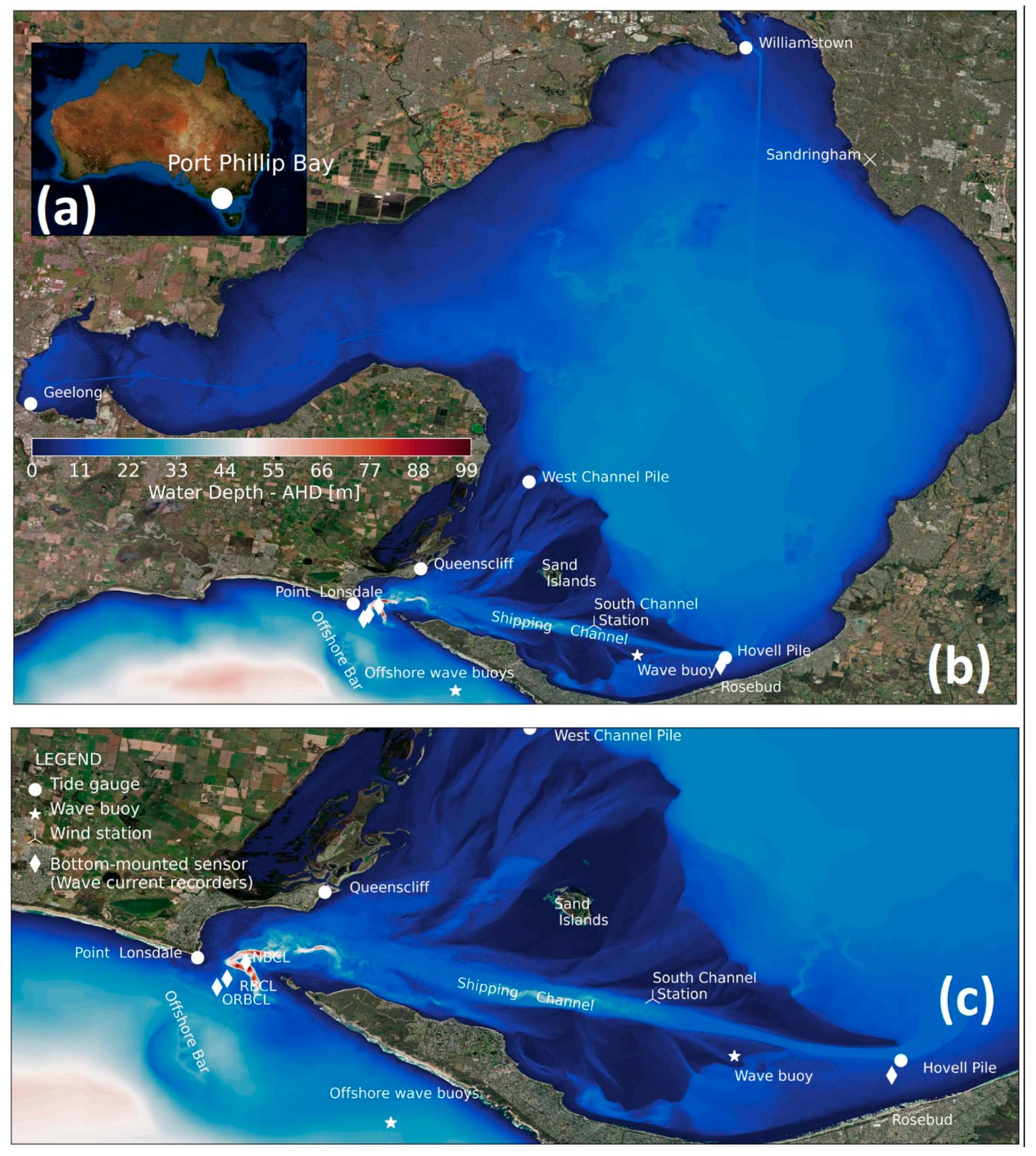
2.1. Field Data

This section describes and analyses observational data available used for the present study. The data included sea levels at tidal gauges, wind, waves and currents. These data were mainly used for model calibration and validation.

2.1.1. Sea Levels

Sea levels within PPB have been observed from several tidal gauges since the 1960s. Measurements were started in 1962 at Point Lonsdale. To date, this station provides up to 54 full years of data, with only one gap longer than one month (between August and November 2012). Another location provided up to 51 full years of records is Williamstown, where the field measurement campaign started in 1966.

Table 1. Observational sea levels in Port Phillip Bay used in the present study.

Station Name	First Operational Year	Number of Full Years
Point Lonsdale	1962	54
Geelong	1965	42
Hovell Pile	1991	26
Queenscliff	1991	23
West Channel Pile	1991	26
Williamstown	1966	51

summaries information about the duration of sea level observations at all tidal stations used for the present study. These stations include Point Lonsdale, Geelong, Hovell Pile, Queenscliff, West Channel Pile, and Williamstown with locations shown in Figure 1. The observed sea levels are hourly data obtained from Tidal Unit—the Australian Bureau of Meteorology (BOM).

An analysis of measured sea levels was undertaken to provide an insight into the magnitude and timing of the largest extreme sea levels in PPB. Figure 2 indicated that Point Lonsdale often experiences a greater extreme level than other locations in PPB due to a larger tidal range induced by ocean tides propagating from the ocean (Bass Strait). However, inside PPB, there is an only minor difference between the extreme sea levels across different stations from Hovell Pile to Geelong. In terms of seasonal variations, the greatest level occurred in winter while the lowest occurred in summer.

It is noted, however, that water levels in PPB have been measured by tidal gauges at an interval of 5 min, which may contain oscillations due to seiches resulting in ‘piling up’ or sudden changes in waters while the present study used hourly data derived from 5-min records by smoothing datasets. Therefore, the actual highest water elevations may be slightly higher than the hourly data.

In terms of timing,

Table 2. Timing of largest “hourly water levels” at tidal gauges in PPB for different seasons.

Station	Summer	Autumn	Winter	Spring
Point Lonsdale	5 January 2014 18:00	26 April 2009 03:00	12 July 1964 05:00	5 November 1994 16:00
Geelong	9 February 1996 21:00	27 May 1994 07:00	29 June 1980 06:00	6 November 1994 20:00
Hovell Pile	2 February 2005 21:00	26 April 2009 07:00	12 July 2016 11:00	6 November 1994 20:00
Queenscliff	5 January 2014 18:00	26 April 2009 04:00	5 July 2011 06:00	7 September 2012 08:00
West Channel Pile	2 February 2005 21:00	26 April 2009 07:00	5 July 2011 08:00	6 November 1994 20:00
Williamstown	9 February 1996 20:00	26 April 2009 07:00	24 June 2014 04:00	6 November 1994 20:00

shows the largest extreme sea levels at many stations from a single event. For instance, during a single storm in November 1994, the maximum sea levels at several stations occurred at the same time at 20:00 on 6 November 1994. However, there is often a time lag between Point Lonsdale and the inner stations. This phenomenon can clearly be seen in autumn and spring. For example, in autumn, the maximum water level at Point Lonsdale occurs 1 h ahead of that at Queenscliff. The time lag is due to travelling time of the peak of astronomical tides from Bass Strait into the Bay.

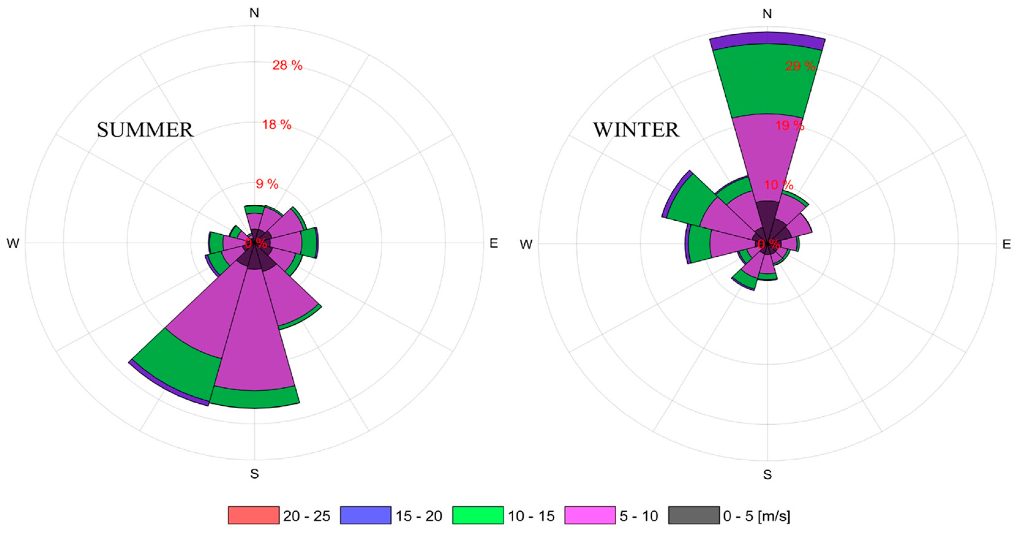
2.1.2. Wind Observations

Measured wind data are very limited in PPB (Cardno Lawson Treloar, [6,16]). The BOM operates two wind stations located at Point Wilson (near Geelong) and the South Channel station. Figure 3 plots two wind roses derived from measured data at the South Channel station from 1998 to 2013 for summer and winter months. In summer, about 50% wind blows from the Southern Ocean towards PPB while in winter, about 40% wind comes from the mainland (e.g., from north). It is noted that Bass Strait and Port Phillip Bay are located on the boundary between the western and the subtropical wind belt [6]. In summer, the trade-wind belt moves to the south with the thermal equator. Further, the mainland regions heat resulting in low-pressure regions. Therefore, wind often blows from the ocean to the mainland during summer months (southerly wind). In winter, the trade-wind belt and pressure patterns opposite to those in summer. Therefore, over PPB, the main wind direction during winter is northerly. In this study, the observed wind data do not provide sufficient spatiotemporal information to serve our purpose to simulate long-term hindcasts because there are many missing values in the data. Further, the field data covers only 15 years, while hindcast simulations are for 27 years. Therefore, the measured wind is only useful for validation such as comparing with wind input for numerical models.

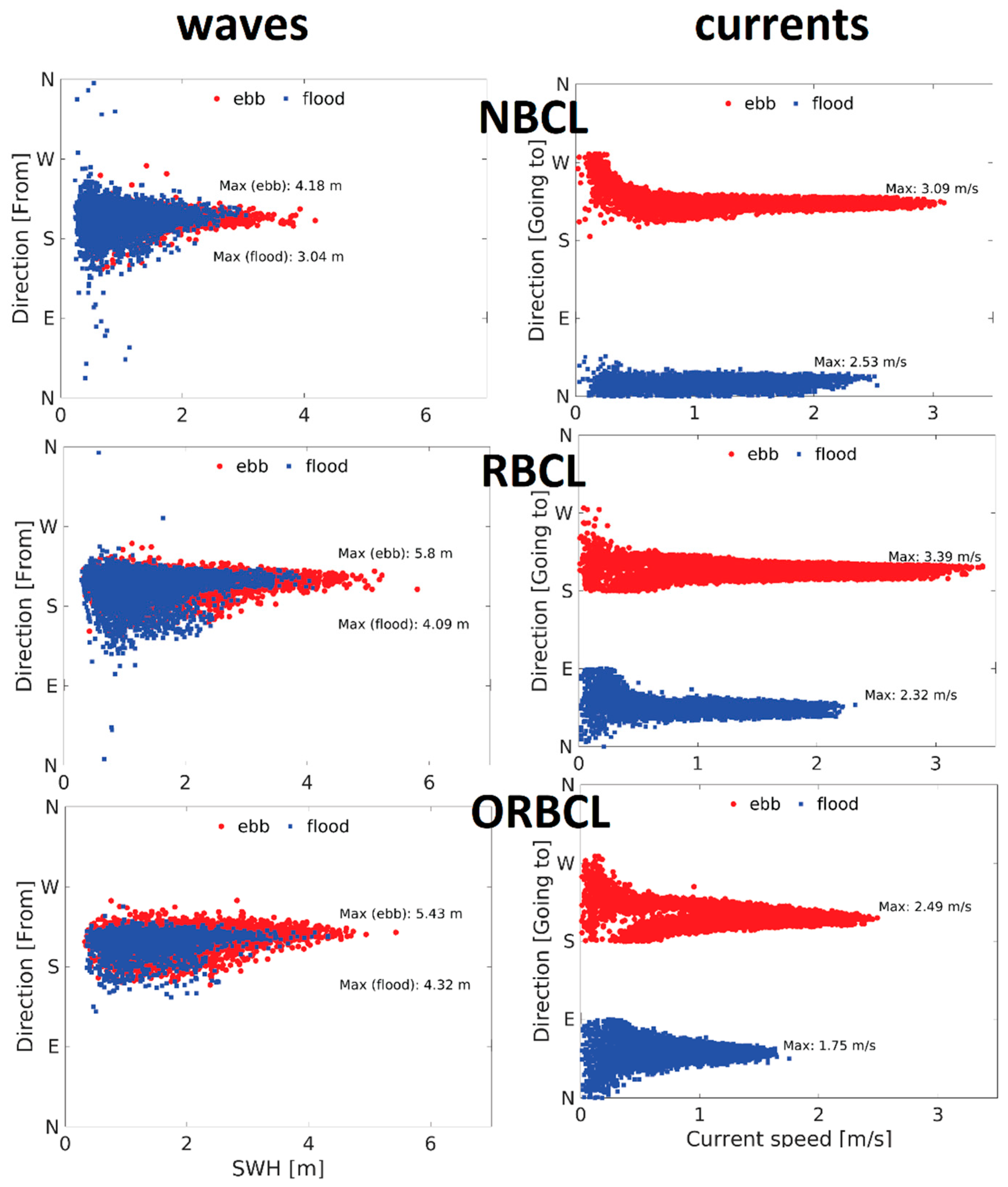
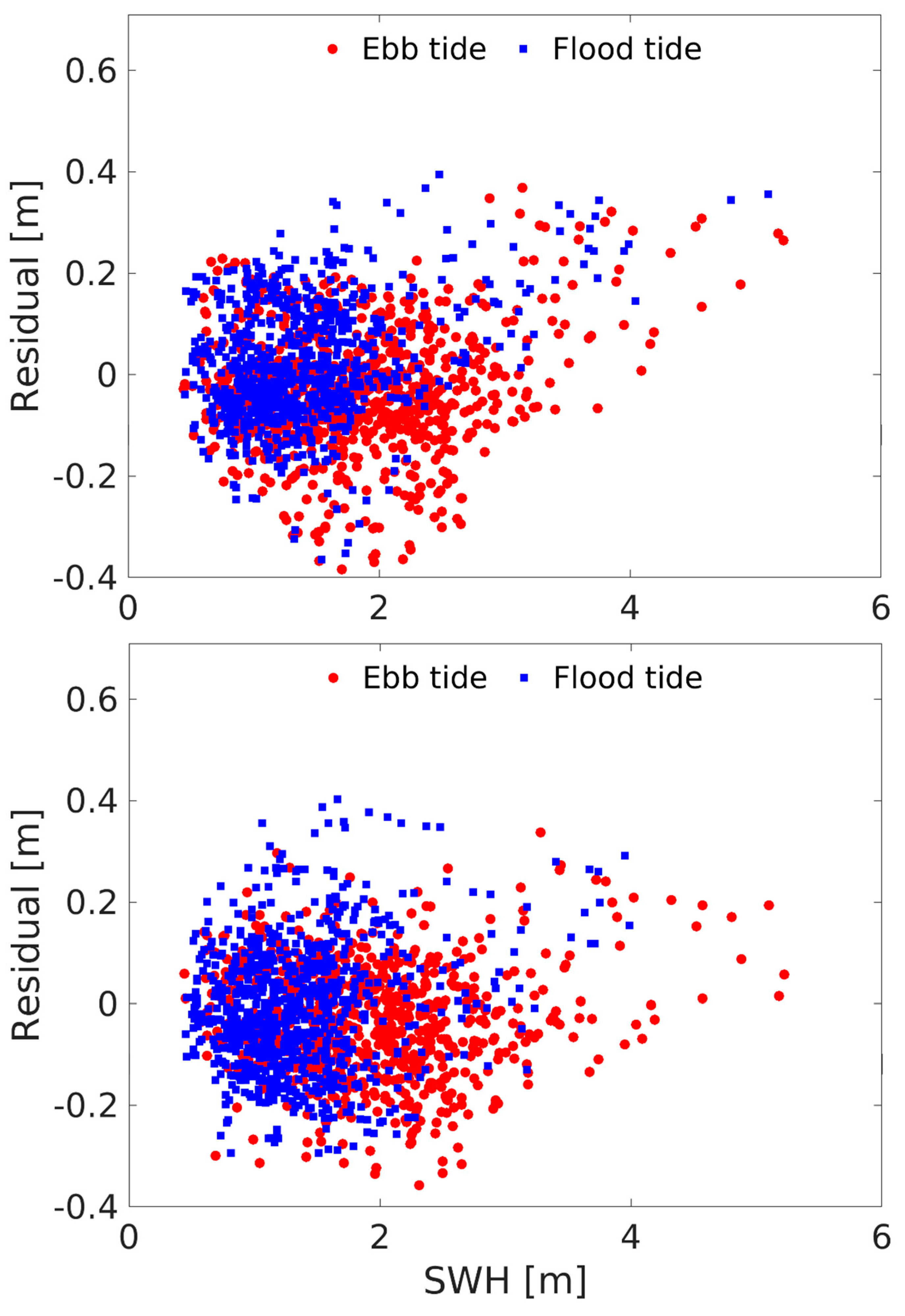
2.1.3. Wave and Current Measurements

At the entrance of PPB, wave and current measurements have intensively been undertaken for many years by Port of Melbourne Corporation (PoMC). For safe navigation, bottom-mounted instruments are often deployed to measure wave and velocity profiles passing this region. Types of bottom-mounted sensors include the acoustic wave and current recorder (AWAC, manufactured by Nortek Group, Vangkroken, Norway) and the acoustic Doppler current profiler (ADCP, manufactured by Teledyne Technologies Company, Poway, CA, USA). The locations of the AWAC and ADCP sensors were not fixed in time; they were moved among a set of fixed sites for operational purposes with the water depth ranging from 15 m to 17 m. As PPH is known to create hazardous conditions for ship navigation, these sensors were deployed to characterize severe sea state conditions. For example, three bottom-mounted sensors were deployed in a straight line along the Great Ship Channel to measure the variability of wave conditions after propagating onto the complex seabed regions around the deep canyon. Due to channel deepening and maintenance works, field measurement campaigns at PPH were often discontinuous, and each deployment often took 2–3 months. Parametric data (waves and currents) were derived from 20 min bursts every hour.

Scatter plots shown in Figure 4 compare the significant wave height (SWH) against the mean wave direction (left panels) and the depth-averaged current speed against the mean current-direction (right panels) with respect to flood and ebb tides. These data were measured by bottom-mounted sensors at three locations (NBCL, RBCL, ORBCL) at PPH between 2006 and 2012. Generally, waves get larger and currents are stronger during the ebb tide than the flood tide. Of the three locations, SWH at RBCL (see the middle point in panel c of Figure 1 for this location) is usually larger than the two other locations as waves interact with strong currents at this point prior to propagating onto the deep canyon to reach NBCL (the inner point). At NBCL, waves reduce their height and lose energy due to breaking. As a result, SWH at NBCL is often smaller than that at RBCL. Measured waves and currents at PPH provide useful information for model calibration and validation, and to investigate the variability of hydrodynamic conditions across both time and space.

Further offshore from PPH, offshore wave measurements using wave buoys have also been intensively undertaken since 1993 by the Victorian Regional Channel Authority (VRCA) and PoMC. Buoys were deployed at the water depth of about 25 m with the location are shown in Figure 1. In the early stage, wave measurements were discontinuous until 2002. From then, waves have been measured using Triaxis buoys, manufactured by Axys Environmental System, Canada. Buoys have three accelerometers, a flux-gate compass and three sensors (angular rate gyroscopic), allowing the measurement of the buoy’s motion and the establishment of the directional wave spectrum. The offshore wave buoy data obtained in the present study covered 15 consecutive years (2002–2016) with minor gaps. The outputs are in both parametric form and 1.5D spectral format with 30 min intervals. All raw data were processed with the aid of the manufacturer’s software and passed quality control processes. The frequency ranges from 0.06 to 0.48 Hz with an interval of 0.005 Hz.

Other than PPH and offshore locations, limited wave and current data are available inside PPB. The only source of data in the inner region was provided by Lawson and Treloar [6]. In 2003, following a request from the PoMC, field measurements were undertaken to record waves generated by vessel movements in the South Channel of PPB. Two Waverider^®® buoys were deployed in the vicinity of the South Channel moored at approximately 2.3 km off Rosebud (see Figure 1) at the water depth of about 11 m. In the present study, these wave data were used to check the wave model performance with different wave physics.

2.1.4. Bathymetry

Bathymetry mapping has been frequently undertaken in PPB with a main focus on the vicinity of shipping channels. The high-resolution bathymetry data used in this study benefited from industry. The main bathymetric data were conducted by Port of Melbourne during summer 2007/2008 and 2009/2010 using several mapping methods, including the laser airborne depth sounding (LADS) and the multi-beam echo sounder (MBES) systems. In PPH, the processed data were in rectangular grids with a resolution of 6.0 m. Along the shipping channel, the resolution is much finer up to 0.5 m. These data are provided by Victorian Ports Corporation (Melbourne, Australia); part of the data was described in Cardno Lawson Treloar [6,16].

2.2. Numerical Models

Numerical models were employed in the present study to replicate hydrodynamic conditions in PPB. This is a complex tidal inlet-lagoon system with irregular bathymetry and shorelines. As PPB hydrodynamics play in a vital role in different physical processes, it requires the utilization of an appropriate numerical modelling framework, which involves in the coupling of a circulation model with a wave model. This coupled system should capture the complexity of coastal shorelines and bathymetry, and physical processes in PPB while it still achieves computational efficiency.

For the reasons above, the present study uses the unstructured grid modelling system SCHISM (Semi-implicit Cross-scale Hydroscience Integrated System) based on Zhang et al. [17]. SCHISM is an upgraded version of the original work done by Zhang and Baptista [18]. This state-of-the-art open-source ocean modelling system is widely used by the scientific community and industry for a range of regional and coastal scale applications such as storm surges, hurricanes and typhoons [19,20,21,22,23]. Details of this modelling framework and related publications can be found at (http://ccrm.vims.edu/schismweb/ accessed on 20 July 2021).

The major feature of SCHISM is that it solves advection in the momentum terms using semi-implicit schemes, resulting in numerical stability, and reducing constraints in time steps (e.g., Guérin et al. [24]). The governing equations in SCHISM include:

$$\mathrm{Momentum}:\frac{dU}{dt}-\frac{\partial }{\partial z} \left(k_1\frac{\partial U}{\partial z}\right)+g\nabla \eta -S=0$$

$$\mathrm{Continuity}:\nabla .U+\frac{\partial w}{\partial z}=0 and \frac{\partial \eta }{\partial t}+\nabla .{{\displaystyle \int }}_{-H}^{\eta }U dz=0$$

$$\mathrm{Transport}:\frac{\partial c}{\partial t}+\nabla .\left(Uc\right)-\frac{\partial }{\partial z} \left(k_2\frac{\partial c}{\partial z}\right)-K_h=0$$

where dU/dt is the time derivative of horizontal velocity U with respect to time t; the free surface η represents the horizontal x, y—Cartesian coordinate system and the vertical coordinate z-direction (up) with corresponding vertical velocity w; H is water depth; k₁ and k₂ represent the vertical eddy and diffusivity, respectively; g is gravitational acceleration and the S term in the momentum equation represents other forces (e.g., tidal, atmospheric forcing). The c term in the transport equation represents the concentration of tracers (e.g., temperature, salinity, sediment transport). These equations are closed using the generic length-scale model proposed by Umlauf and Burchard [25]. At the first computational step, SCHISM solves the momentum and transport equations using the semi-implicit finite element method. The implicit scheme is applied to solve the elevation gradient, vertical viscosity and boundary layer and the divergence terms. Thus, stability constraints (e.g., large time step) can be obtained using this numerical scheme. After solving the horizontal velocity and elevation, the vertical velocity is computed using the finite volume method along each prism. SCHISM can directly be coupled with the spectral WWMIII model introduced by Roland et al. [26]. This is a third-generation phase-averaged, unstructured grid wave model that allows to compute the wave spectra over realistic coastal and ocean regions. From spectral information, key wave parameters such as wave height and direction can be extracted. WWMIII solves the wave action balance equation, which accounts for various physical processes such as wind energy and dissipation due to white-capping and bottom friction. As a phase-average wave model, it is noted that WWM only considers refraction and diffraction, not reflection. The governing equation reads as follows:

$$\underset{time space}{\underbrace{\frac{\partial A}{\partial t}}}+\underset{geographical space}{\underbrace{{\nabla }_s\left[\left(c_g+U\right) A\right]} }+\underset{spectral space}{\underbrace{{\nabla }_k \left[c_k A\right]} }=\underset{source/sinks}{\underbrace{\frac{S}{\omega }}}$$

where A represents the action density as a function of intrinsic radian frequency ω and wave number k, written as:

$$A=\frac{E \left(\omega ,k\right)}{\omega }$$

In the linear wave theory, temporal and spatial scales of the wave field obey the “dispersion relationship”; g accounts for the gravitational acceleration; H is water depth, and c_g is wave group velocity. In the presence of a current, the current speed U can modify the wave propagation. ∇ operators represent the geographical divergence (horizontal) and spectral space (with subscript k). The S term represents the energy of various source/sink terms such as wind forcing, white-capping and bottom dissipation. In WWMIII, the geographical space is solved with the residual distribution scheme, which incorporates the advantages of both finite elements and finite volume methods (e.g., Roland et al. [26]). The spectral space is integrated using the UQ method—a similar method as that in WW3 [27]. The source terms are solved in three fractional steps using the TVD Runge–Kutta method, which is a third-order scheme applied for dissipation terms (e.g., bottom friction, breaking), a dynamic scheme for nonlinear interaction (e.g., triads) and a semi-implicit scheme for deep-water source terms. The coupling system have been paralleled using MPI (Message Passing Interface) with identical sub-domains decomposed from the same unstructured grid, but with the user-defined time steps. Therefore, this coupled modelling system has no grid interpolation error. Further, this coupled system provides computational efficiency because each model component can be set with a different timestep using various integration schemes.

Furthermore, the WWMIII module used in the present study was integrated with the advanced wave physics including the upgrade of wind source and wave dissipation terms (ST6), which were benefited from a study done by Tran [15]. This advanced physical package was derived from many years studying wind-wave physics (e.g., Donelan et al. [28,29]; Babanin et al. [30]) and observations. In wave modelling, ST6 was based on the original work done by Roger et al. [31] in SWAN, and Zieger et al. [32] and Liu et al. [33] in WW3, which have shown improvements in predicting waves across different scales ranging from coastal areas to deep oceans (e.g., see Roger et al. [26], Zieger et al. [32], and Liu et al. [33] for more detail). All of the key features mentioned above make the coupled SCHISM-WWMIII system highly efficient for simulating hydrodynamics in PPB including wave-current coupling.

2.3. Model Setups

SCHISM-WMM modelling system requires a computational mesh with forcing inputs and boundary conditions for each model component. A detailed description is presented as follows.

2.3.1. Computational Mesh

In the present study, a same unstructured mesh was used for both SCHISM/WMM. This mesh has 54,432 nodes with 103,543 elements. The grid resolution ranges from about 20 m within PPB to 3 km at furthest points offshore. The finest mesh was focused on the region of interesting physics at PPH where the bathymetry and hydrodynamic patterns are complex. The open boundary of the computational domain is extended about 200 km offshore from PPH at deep water to capture ocean tides and waves.

2.3.2. SCHISM Model Forcing and Boundary Conditions

The open boundary was forced with ten tidal constituents (Q1, O1, P1, K1, N2, M2, S2, K2, SA, SSA) using the latest version of the global finite element solution tide model—FES 2014 (Carrere et al. [34]) produced by Noveltis, Legos and CLS and distributed by AVISO+, with support from Cnes (https://www.aviso.altimetry.fr/ (accessed on 5 March 2020)), which includes improvements in grid resolutions, especially in coastal regions and the continental shelf with new global bathymetry. FES 2014 was assimilated with long-term altimeter data from Envisat, TOPEX/Poseidon, Jason-1, Jason-2, TPN-J1N, ERS-1 and ERS-2 and field measurements at various tidal gauges. The distributed FES 2014 database provides a high resolution of 1/16⁰, which is 50% finer than the FES 2012 model. Additionally, SCHISM allows the inclusion of several atmospheric parameters: wind, air pressure, temperature, specific humidity, and fluxes of short and long waves. These forcing terms are in NETCDF formats. Within PPB, except for wind field, none of these parameters are available. Though available, measured wind data within the study domain was not continuously recorded. Therefore, for the purpose of long-term hindcasts, data from global atmospheric models were used to force the SCHISM model. Particularly, the present study uses the finest (e.g., 0.25⁰ resolution) hourly atmospheric forcing CFSR data provided by NCEP, which were derived from the coupled atmospheric-ocean-land-surface-sea-ice modelling system with the aid of assimilation techniques [35,36]. The selection of CFSR came after comparing both CFSR and ERA5, which is the latest ECMWF products with the field data at the South Channel station. CFSR wind provides a better agreement with the field data than ERA5, which underestimates the high wind speed (see Figure 5). Further, SCHISM was also forced with non-tidal signals produced by HYCOM models (https://www.hycom.org/ (accessed on 5 March 2020)) without the effect of sea level rises.

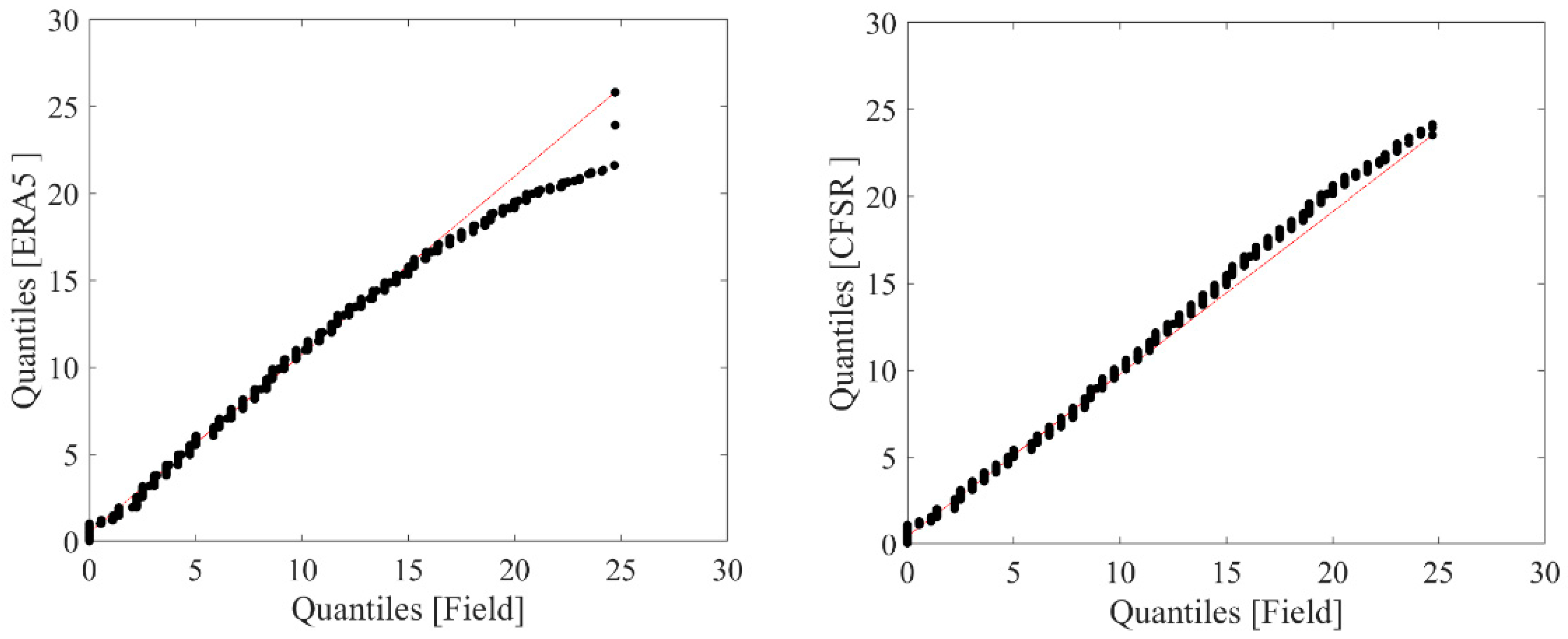
2.3.3. WMMIII Model Forcing and Boundary Conditions

WWMIII also applied the same atmospheric forcing inputs as those used for the SCHISM model including wind and pressure fields. The WWM open boundary was prescribed with the ocean waves from WW3 hindcast data provided by the French Research Institute for Exploitation of the Sea (IFREMER; ftp://ftp.ifremer.fr/ifremer/ww3/HINDCAST (accessed on 5 December 2019)) [37]. This data source can provide up to 30 years of data at 0.5⁰ resolution and 3-hourly intervals in parametric formats that can be directly read by WWMIII.

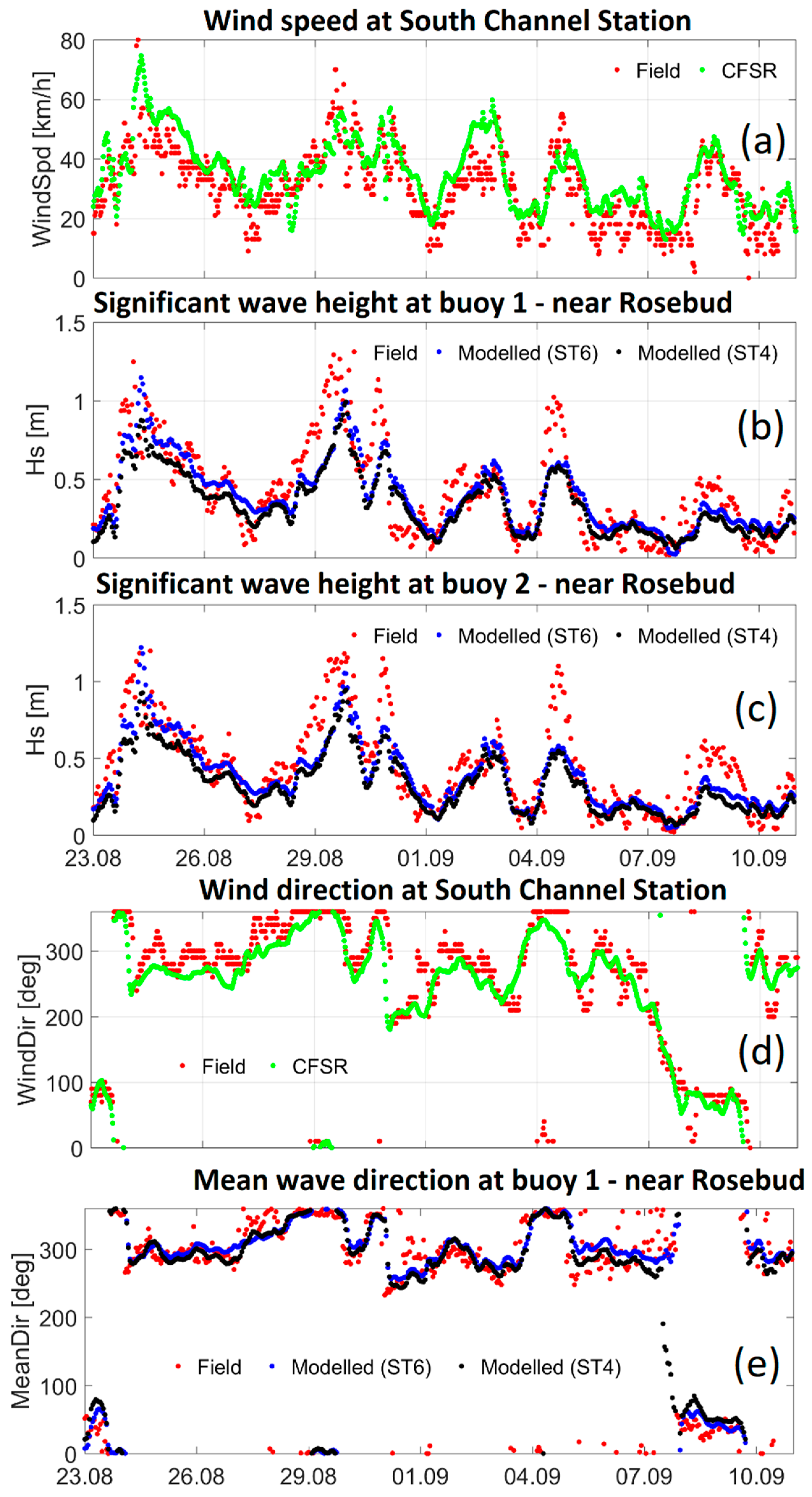
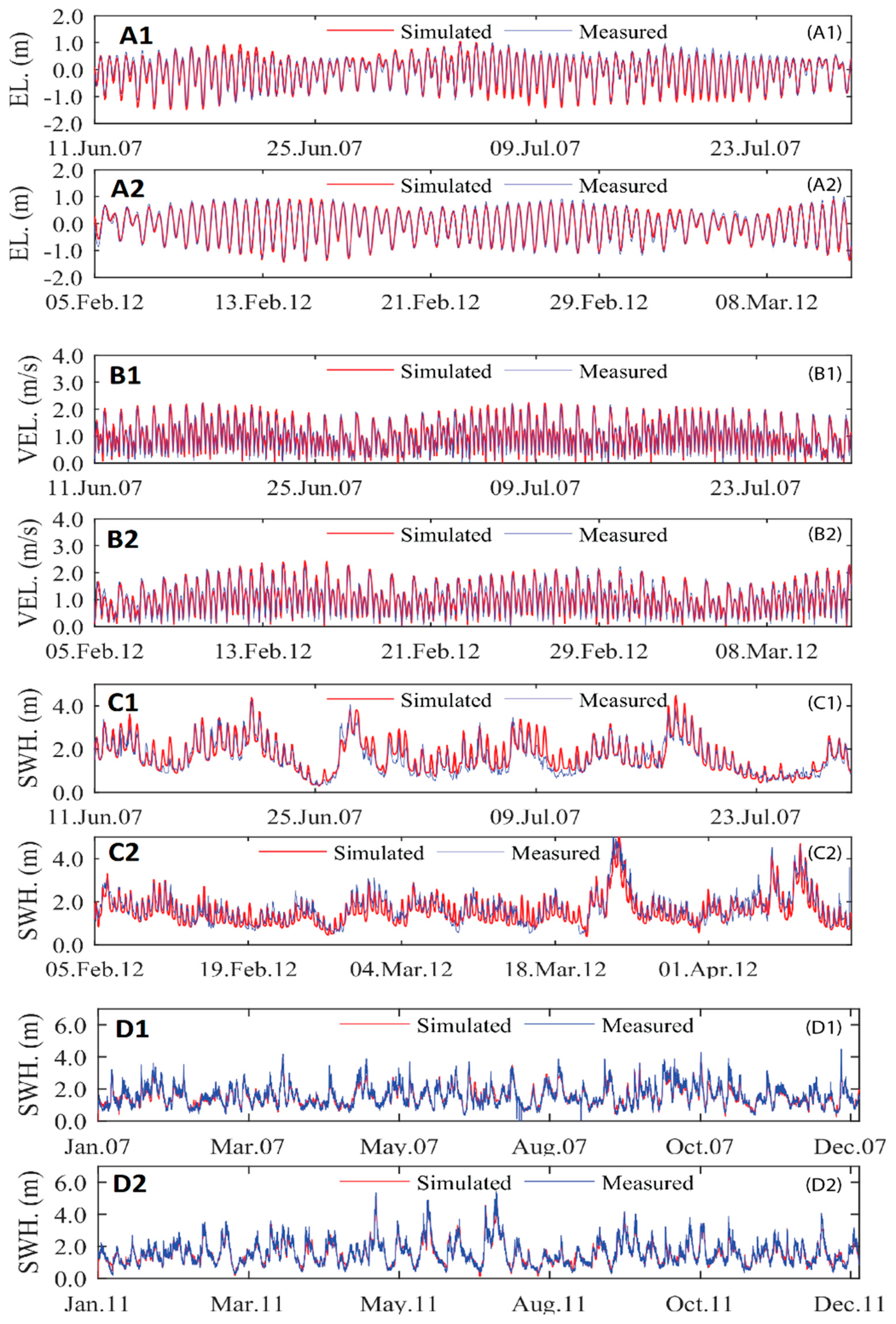
2.4. Model Calibration and Validation

In practice, model calibration and validation are important processes. The purpose of model calibration is to adjust model configurations to optimize the model performance. Usually, the model accuracy can be determined by comparing modelled results with the field data available. Validation comes afterward using the same configured settings in the calibration process, but testing for a different period.

For SCHISM, the present study tested several bottom friction formulations including Manning and drag formulas. Following several short simulations to examine the model stability, the quadratic drag formulation was chosen as other formulations (e.g., Manning) produced noise. Once the drag formulation was selected, the coefficient was adjusted to obtain reasonable agreement between the model solutions and the field data. During the calibration, different time steps were also tested. To this end, a time step of 120 s was chosen for SCHISM. For simplicity, the final calibration of SCHISM with a same drag coefficient of 0.002 (quadratic formulation) was applied to every grid point in the computational domain. Once the coefficient was chosen in the calibration step, the calibrated configuration was applied to validate SCHISM by running the model over a different period (e.g., another month). For WWMIII, the wave model was firstly simulated without imposing a current and water level. This step is to ensure ocean waves are well replicated by WWMIII. To demonstrate the model performance, field data at offshore buoy locations were used for calibrating and validating WWMIII because waves at this location are generally not affected by currents. A final timestep of 360 s was selected for WWMIII. After that, SCHISM was fully coupled with WWMIII to replicate the hydrodynamics at PPB. This coupled system is especially important for PPH where waves interact with strong tidal currents. Further, as mentioned, WWMIII in this study was configured with ST6 physics. The calibration and validation of WWIII model was benefited from the work done by Tran [15] with testing undertaken for various water environments including PPB. Although ST6 calibration and validation are not detailed here, timeseries plots derived from ST6 validation for PPB waves are also provided in Figure 6.

Other than that, main calibration and validation of SCHISM/WWMIII are focused within PPH (waves, currents), offshore waves and water levels at 6 locations in PPB. Model performance was evaluated using skill metrics with several statistical parameters as shown in

Table 3. Model skill assessments.

Bias	$BIAS=\sqrt{\frac{{\displaystyle \sum }{\left(X_f-\overline{X_f}\right)}^2}{N}}-\sqrt{\frac{{\displaystyle \sum }{\left(X_m-\overline{X_m}\right)}^2}{N}}$	(A-1)
Correlation	$R=\frac{{\displaystyle \sum }\left(X_f-\overline{X_f}\right)\left(X_m-\overline{X_m}\right)}{\sqrt{{\displaystyle \sum }{\left(X_f-\overline{X_f}\right)}^2{\displaystyle \sum }{\left(X_m-\overline{X_m}\right)}^2}}$	(A-2)
Coefficient of determination	$R^2=1-\frac{{\displaystyle \sum }{\left(X_f-X_m\right)}^2}{{\displaystyle \sum }\left(X_f-\overline{X_f}\right)}$	(A-3)
Root mean squared error	$RMSE=\sqrt{\frac{{\displaystyle \sum }{\left(X_f-X_m\right)}^2}{N}}$	(A-4)

Where $X_m$ is modelled data, and $X_f$ presents field measurements.

.

Figure 7 shows time series plots that compare the measured and field data at ORBCL obtained during the calibration and validation of SCHISM for water level (A1, A2 panels) and current speed (B1, B2 panels). It also compares modelled SWHs and buoy data derived from WWM model alone in D1, D2 panels. For coupled SCHISM/WMM, comparisons of the modelled SWH and field data at ORBCL are shown in C1, C2 panels. Several statistics are presented in

Table 4. A statistical summary for model calibration and validation.

LOC	VAR	June and July 2007				February and March 2012
		COR	R2	RMSE	BIA	COR	R2	RMSE	BIA
ORBCL	EL	0.97	0.9	0.17	0.03	0.98	0.94	0.013	0.01
	VEL	0.94	0.87	0.19	0.01	0.92	0.85	0.21	−0.01
	SWH	0.91	0.8	0.33	0.01	0.87	0.72	0.38	−0.04
RBCL	EL	0.97	0.9	0.17	0.03	0.98	0.94	0.13	0.01
	VEL	0.96	0.91	0.21	−0.08	0.97	0.87	0.26	−0.11
	SWH	0.92	0.82	0.32	0.03	0.89	0.77	0.34	−0.04
NBCL	EL	-	-	-	-	0.98	0.94	0.1	0.01
	VEL	-	-	-	-	0.96	0.92	0.19	−0.05
	SWH	-	-	-	-	0.87	0.59	0.34	0.06
LOC	VAR	2007 (full year)				2012 (full year)
		COR	R2	RMSE	BIA	COR	R2	RMSE	BIA
OFFSHORE	SWH	0.91	0.82	0.28	−0.08	0.94	0.89	0.26	−0.07

. As shown, both SCHISM and WWMIII replicate the field data well with a high correlation and low biases. Thus, this coupling system can confidently be used for long-term simulations.

2.5. Long-Term Simulations

SCHISM was configured in depth-averaged (2DH) barotropic modes. This module was coupled with WWMIII using ST6 physics. The time step used in SCHISM was 120 s while WWMII used a time step of 360 s. Long-term simulations were undertaken for 27 years from 1990 to 2016. The model output interval is every two hours for both SCHISM and WWM. The purpose of selecting the two-hourly outputs is to ensure the computational efficiency. More importantly, the two-hourly interval is not too large because a larger output interval may not capture the peak of storms. All simulations were undertaken on University of Melbourne’s High-Performance Computing (HPC) systems.

3. Results

The following sections present results obtained from a spatial analysis of long-term hindcast data focusing on sea levels, waves and currents. For sea levels and waves, the focus is on seasonal variations and return periods. For currents, the focus is on seasonal variations. Further, where relevant and available, the measured data and modelling case scenarios are also used to better understand the hydrodynamics in PPB.

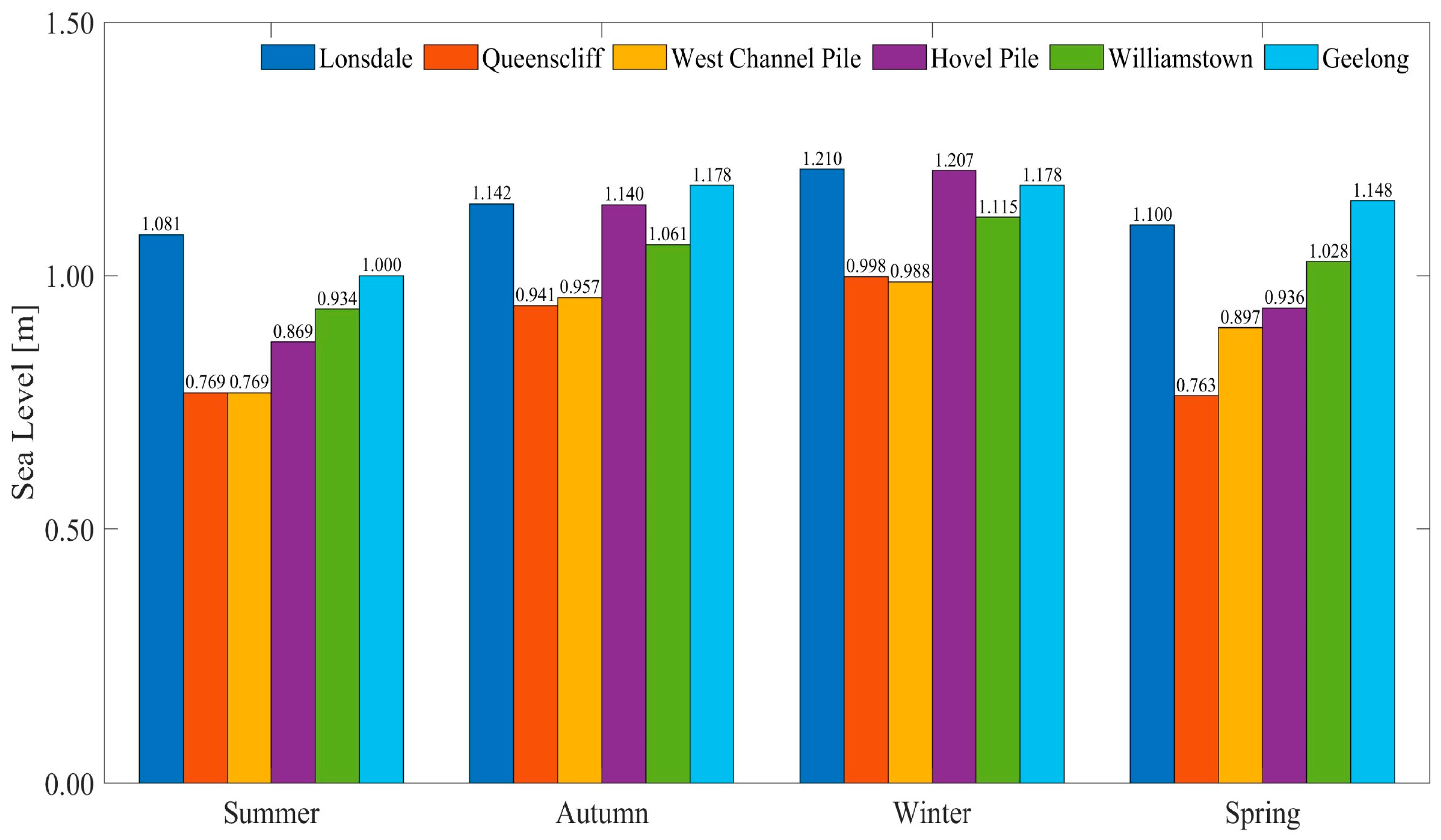
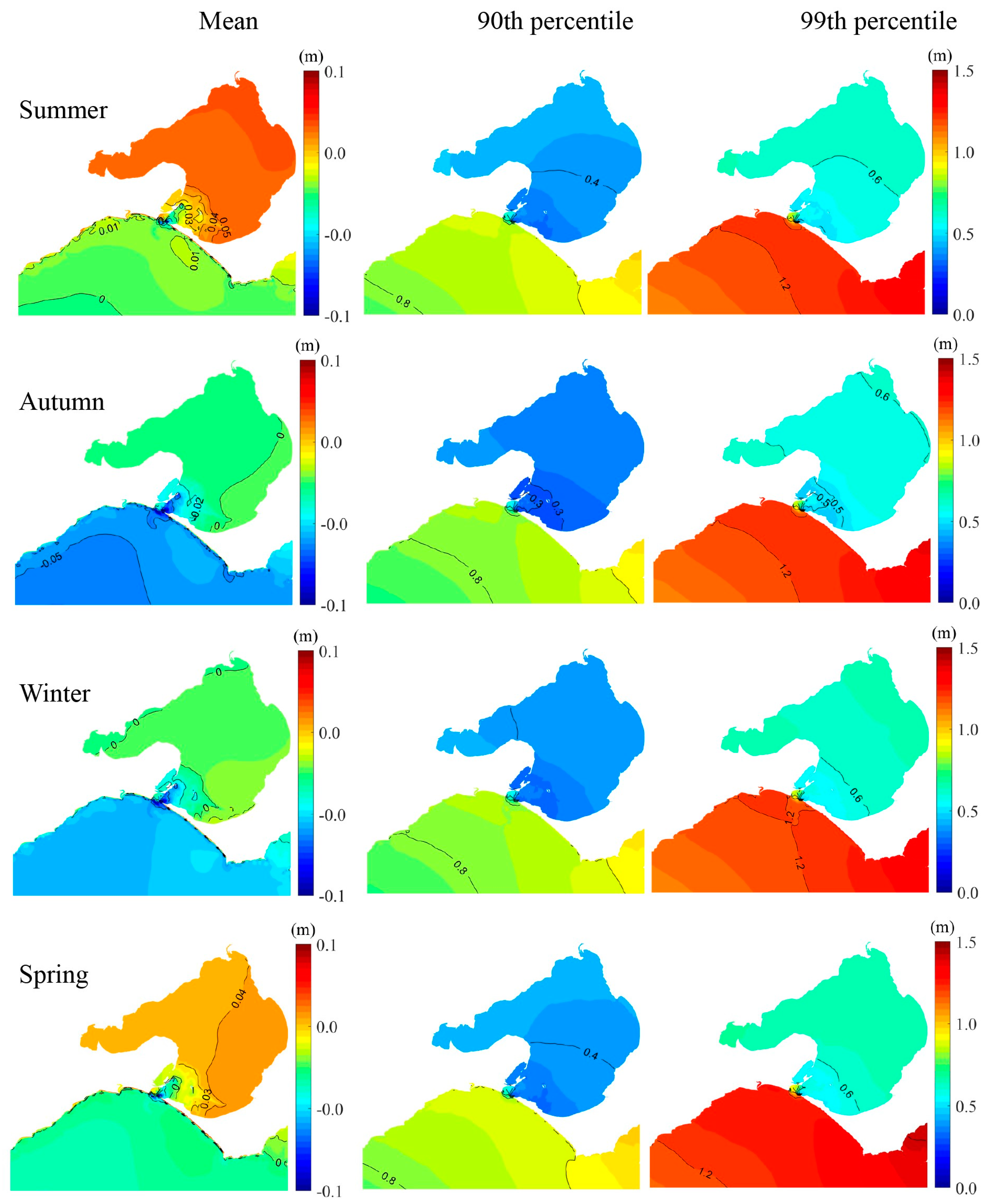
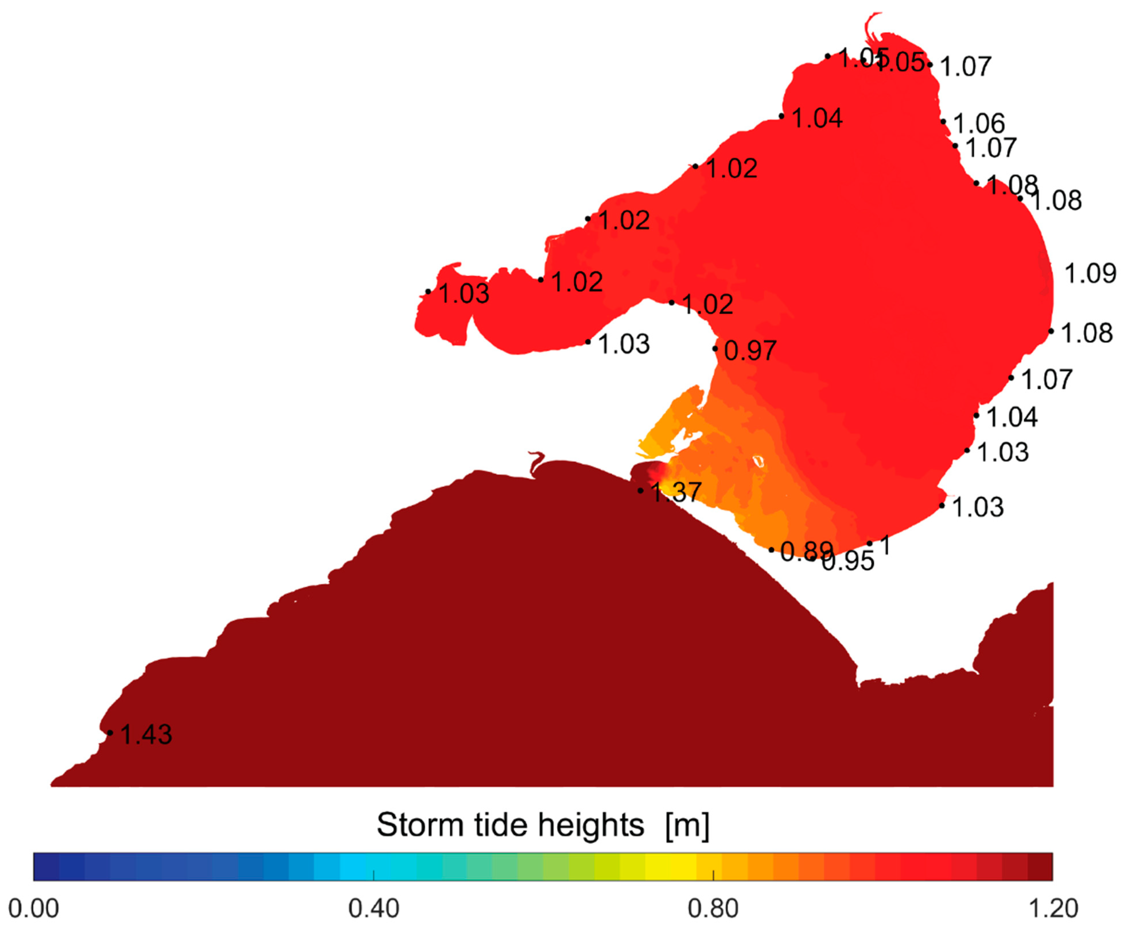
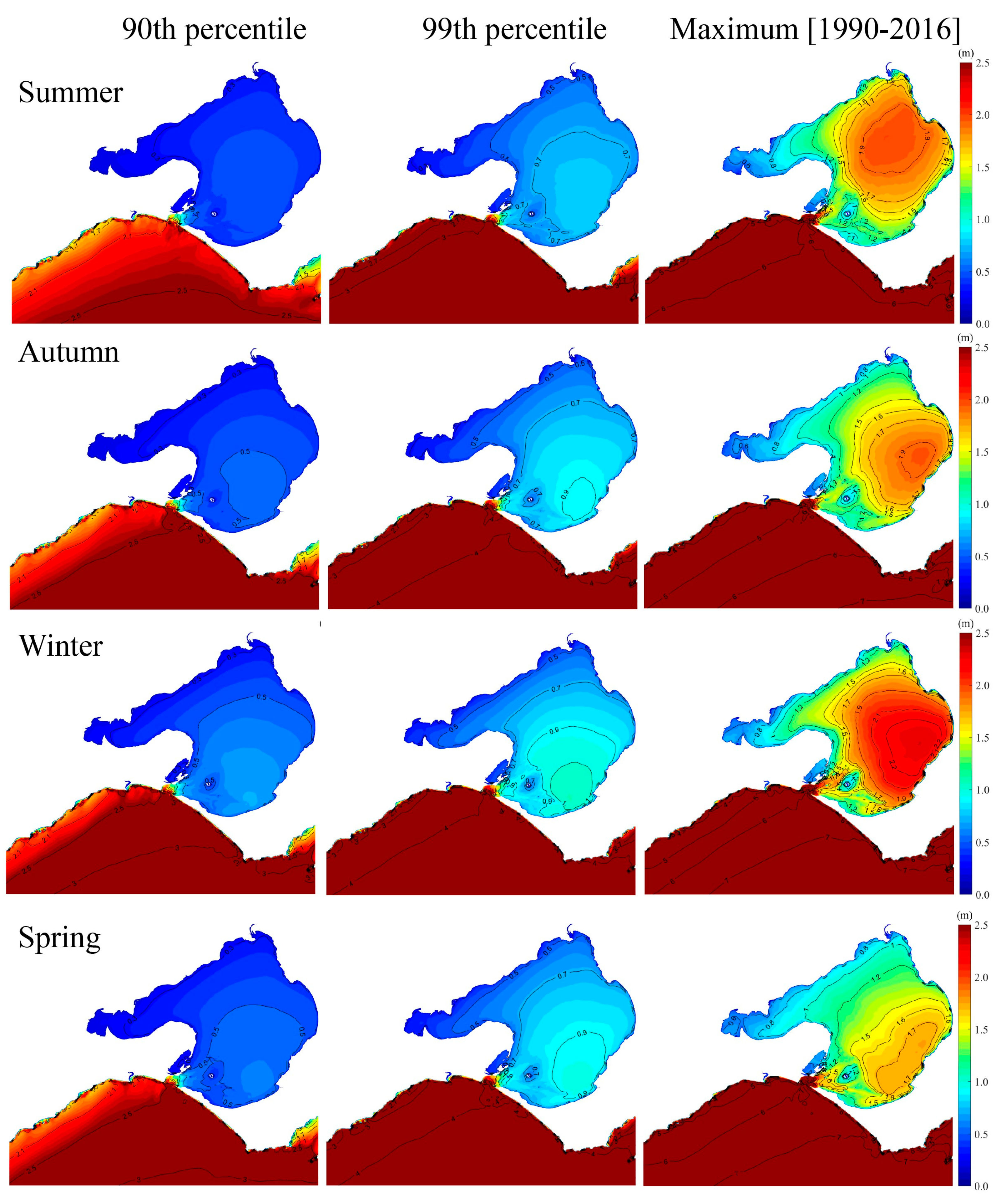
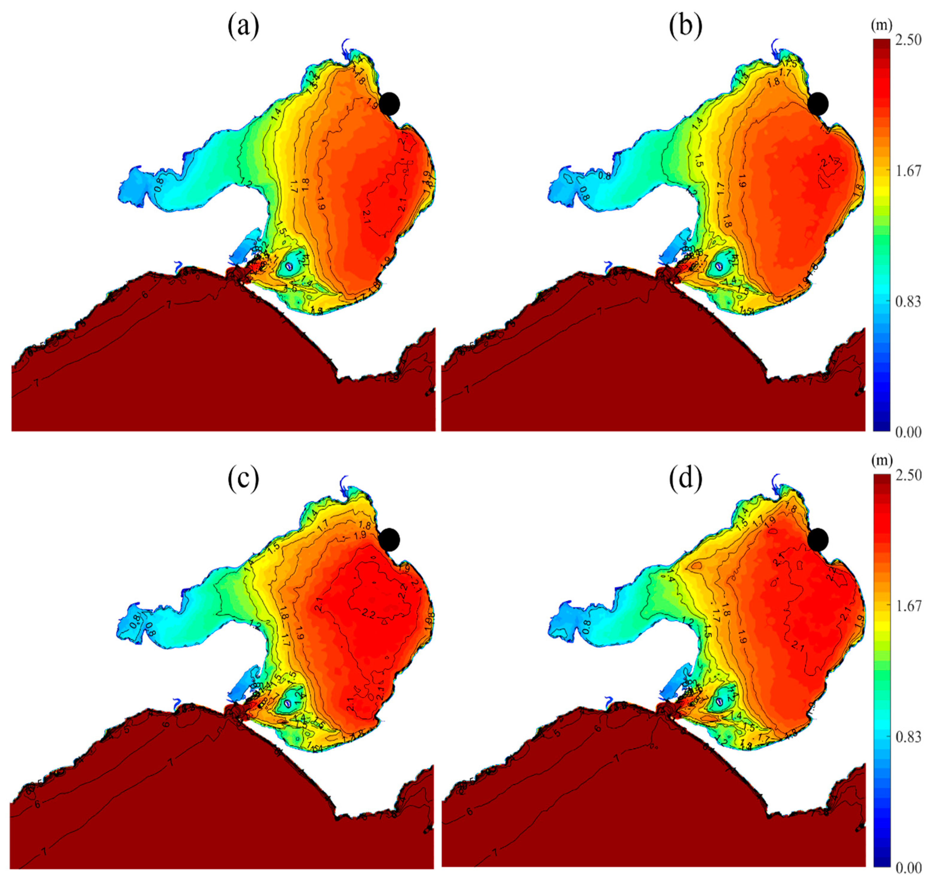
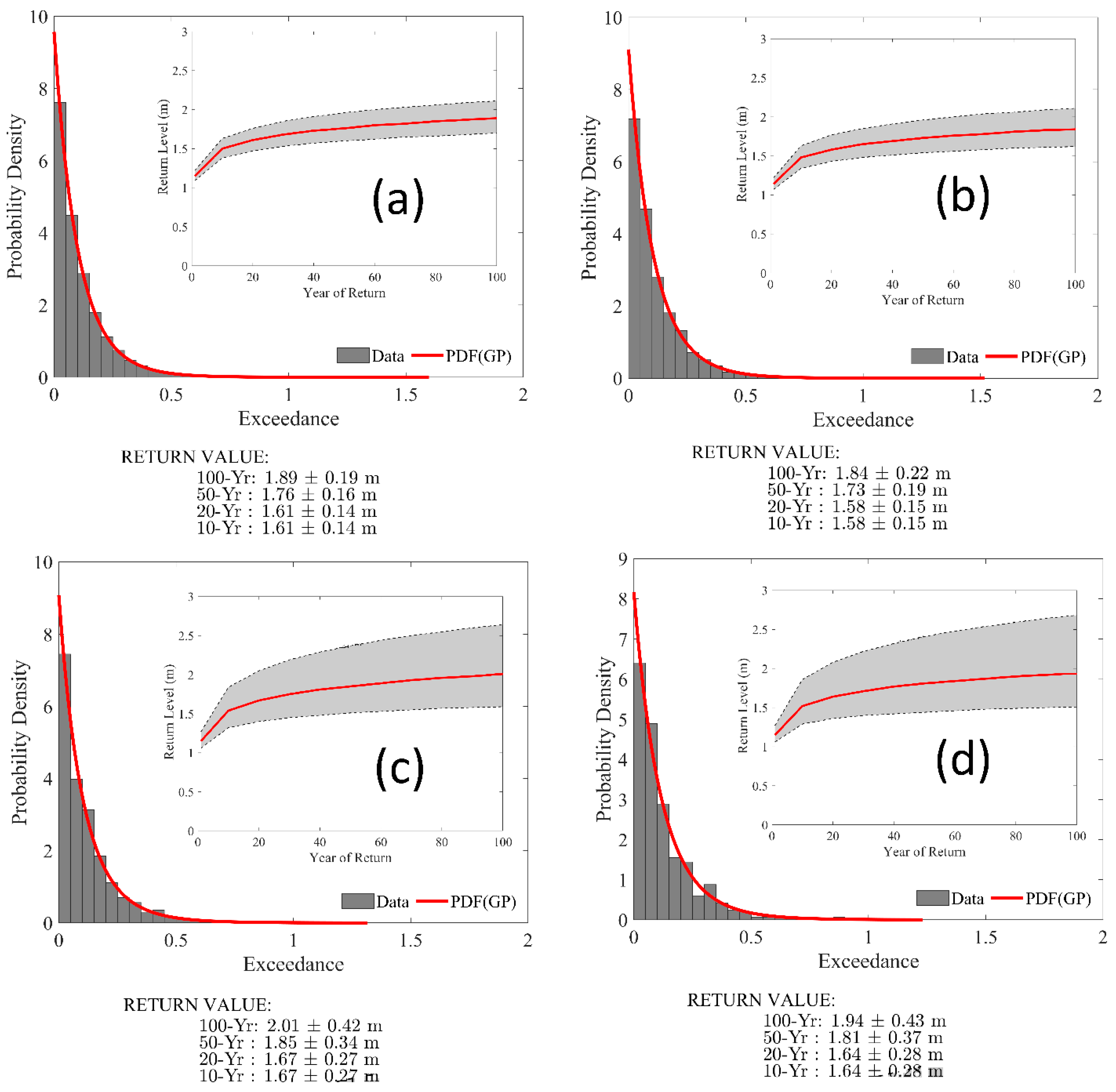
3.1. Seasonal Variations and Return Periods of Sea Levels

Figure 8 presents spatial variations in sea levels across different seasons for the mean value (MSL), 90th and 99th percentiles derived from 27 years of hindcast simulations (1990–2016). For the mean values, a clear picture emerges—the MSL inside PPB is always higher than that outside, regardless of seasonality. For instance, in summer, the MSL inside PPB is higher than offshore, ranging from 3 cm in the southern portion of PPB to 5 cm in the north. There are many mechanisms in the earth’s system to have an effect on MSL. For instance, due to temperature, the ocean water is warmer in summer months than in winter months and the thermal expansion also differs from one season to another. As a result, the MSL in the summer is often higher than in the winter (e.g., Cazenave et al. [38]). For PPB, the highest MSL in spring occurs on the eastern coasts of PPB, while the highest MSL in summer moves further to the north. This suggests that the atmospheric system may affect the MSL pattern in PPB. For example, as shown in the wind-roses presented in Section 2.1.2, the prevalent wind direction in summer is southerly as the land becomes low-pressure regions. Further, the southerly wind blowing to the north can also generate waves resulting in wind-wave setup (e.g., Guérin et al. [24]) that can also increase the mean sea level. For higher percentiles, the water level inside PPB is also lower than outside in line with the narrow entrance where the ocean tides are distorted and filtered out (e.g., see DiLorenzo [39]). However, the seasonal variability of the 90th and 99th percentile water levels is unclear because these levels do not necessarily reflect extreme sea levels in PPB. For example, the 90th percentile level represents the threshold at which 90% of data falls below this level. On average, the 90th percentile water level can occur in PPB on daily basis because it is among 11,800 events (e.g., 10% × 27 years × 365 days × 12 steps) over 27-year hindcasts (~9855 days).

Previously, the 90th percentile sea levels in PPB have been reported based on the observational data at tidal gauges.

Table 5. Comparisons between the 90th percentile sea levels at several stations in PPB estimated Cardno by for ABM [40] and by the present study.

Station	ABM (2015)				Present Study
	Min		Max		Min		Max
	90th	Year	90th	Year	90th	Year	90th	Year
Queenscliff	0.222	1997	0.406	2013	0.300	1997	0.390	2016
Hovell Pile	0.265	1995	0.510	2013	0.300	1995	0.430	2013/16
Williamstown	0.176	1967	0.425	2013	0.360	1997	0.424	2013/16
Geelong	0.260	1971	0.460	1989	0.350	1997	0.449	2016

compares the 90th percentile water levels at several stations estimated by ABM [34] based on yearly observational data with those done by the present study based on hourly field datasets. Despite a few (slightly) differences in values, there are several interesting patterns that are worth mentioning here. Firstly, in both studies, the highest recorded 90th percentile sea levels occurred in 2013 at least three stations, except for the year 2016, which was not included in ABM [40]. Secondly, a major pattern in the 90th percentile sea levels in Table 5 is that the level at Geelong is higher than at Williamstown, while the level at Queenscliff is lower than at Hovell Pile. The 90th percentile water level at Geelong is higher than that at Williamstown, which can be explained by the fact that the 90th percentile threshold is relevant to high-tide waters, which would daily occur during a flood tide. Specifically, during a flood tide, PPB acts as a storage water system as the ocean tides propagate from the ocean into PPB and towards Williamstown and Geelong. However, Geelong is a narrow region and relatively far from the entrance of PPB. Therefore, the water level could be raised for a longer period than at Williamstown and the reversing time occurred between a flood and an ebb tide at Geelong is also longer than at Williamstown. The reason behind the 90th percentile level at Queenscliff is lower than that at Hovell Pile is not clear. ABM [40] speculated that this may be due to the difference in tidal ranges in these two locations. Finally, it is noted in Table 5. That the lowest recorded 90th percentile sea levels in ABM [40] included two unusually low values: 0.176 m in Williamstown in 1967 and 0.26 m in Geelong in 1971. These values were not included in the period of hindcast data used in the present study.

For the 99th percentile threshold, on average, this level reflects ‘one-week’ largest events because there are about 1182 events (e.g., 1% × 27 years × 365 days × 12 steps) in 27-year hindcasts (~9855 days). Therefore, the 99th percentile values do not necessarily reflect the extreme sea levels in PPB. Like the 90th percentile, the 99th percentile sea level inside PPB is also lower than that outside. The most notable feature is that, after passing the Sand Islands, the water level of the entire PPB is nearly the same from Hovell Pile to Williamstown. This indicates that the tidal range in PPB is almost identical over a large portion of the bay.

For return levels, this study estimated the several return levels of storm tides, which took into account the effect of tides + surges + waves using the Peak Over Threshold (POT). A description of this method is given in Appendix A. Figure 9 plots the 100-year return values of storm tides (other lower return levels are not shown). Several interesting patterns emerge from this figure. Firstly, there are only minor differences in the storm tide levels across different locations suggesting the extreme sea levels over the Bay are almost the same. This pattern is also found previously in an analysis of observational sea levels at tidal gauges in Section 2.1. Secondly, the largest 100-year storm tide level in PPB is found on the eastern coasts of PPB in line with the wind pattern. For example, the frontal low weather system often results in the wind blowing from west to east, which can generate larger waves along the eastern side of PPB. This would increase extreme sea levels such as due to wave-setup along this coastal area. Another interesting pattern is that the return values of storm tides in the southern portion of PPB (from the entrance to Great Sand islands) are lower than other regions inside PPB. This pattern is expected due to wave decay from bottom friction and wave breaking resulting in less setup with the entrance area. “Wave-setup at the entrance” phenomenon has been investigated by several authors (e.g., Dunn et al. [41], Hanslow et al. [42]). It can be identified by comparing tidal anomaly from measured water levels with wave heights. To provide evidence, this study plots the relationship between SWHs and tidal residuals at RBCL based on both modelled and measured data in Appendix B (Figure A2), which shows a reduction in tidal residuals when the significant wave height increases.

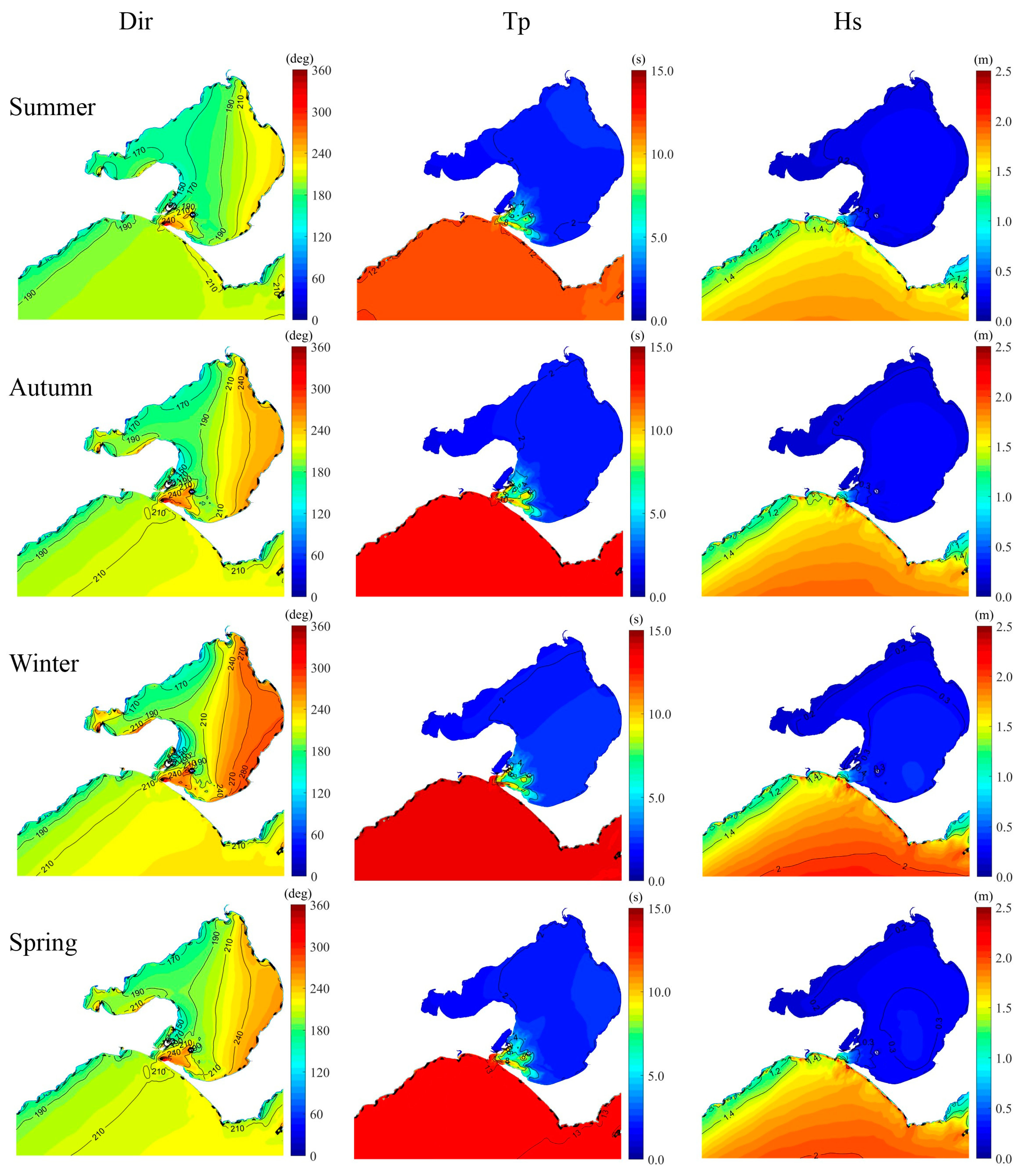
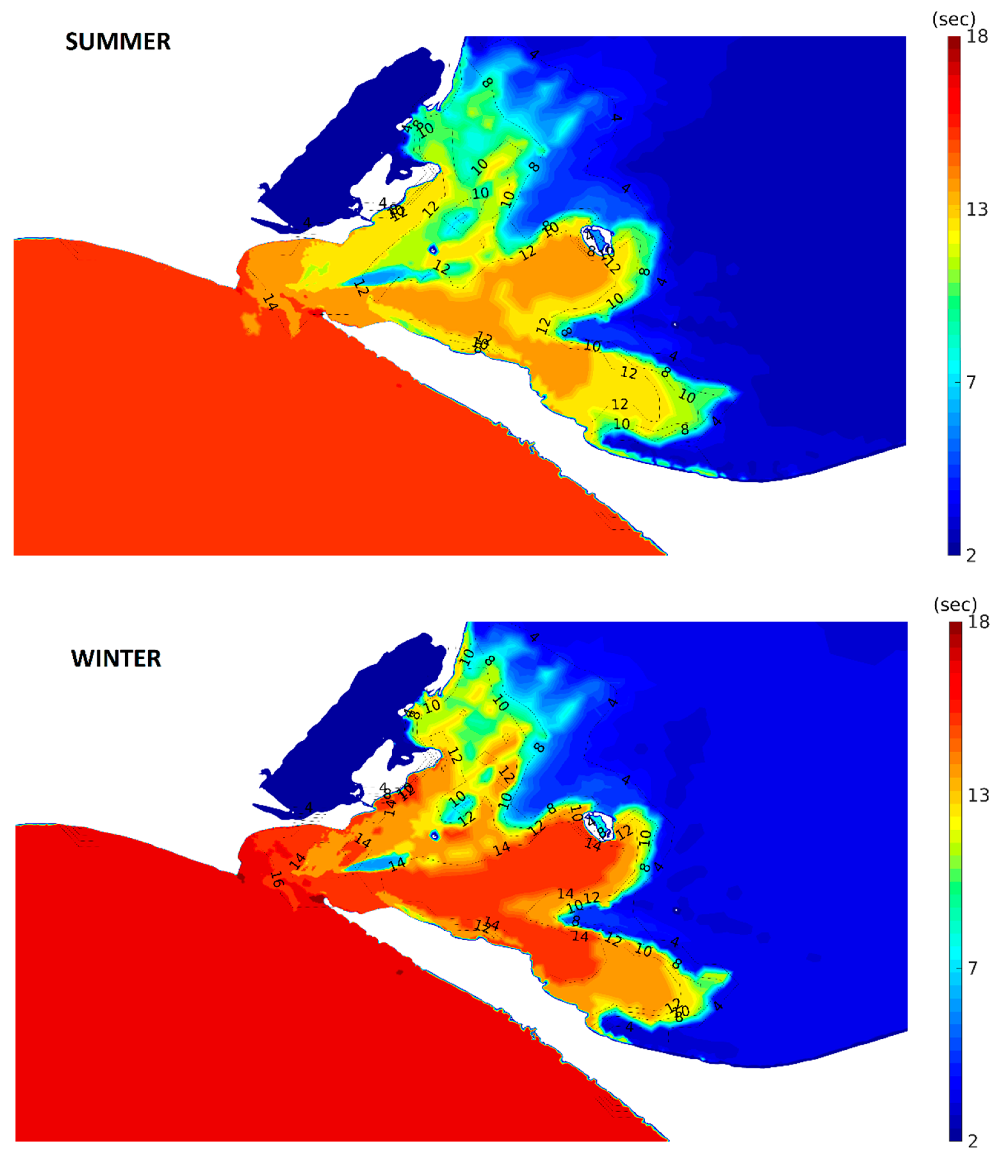
3.2. Seasonal Variations and Return Periods of the Wave Field

Figure 10 shows the spatial variability in the mean value of SWH, mean wave direction and peak period. The mean value was calculated for each season by averaging over 27-year hindcasts. Inside PPB, the wave field is strongly linked with the wind climate. For wave direction, the predominant direction in summer over a half of PPB is between 180⁰ and 210⁰. Thus, waves mainly propagate from the south towards the north. This is a predominant wave direction because in summer the most prevalent winds are south-westerlies (e.g., Cardno Lawson Treloar, [6]). The opposite wind pattern is true during winter. Specifically, the prevalent winds in winter are northerlies. Therefore, wave propagate further to the south from the north. At the entrance, Figure 10 shows an evidence of refracted waves. This can be seen in the area covered with the mean wave direction of 240⁰ within the inlet area getting larger in winter compared to summer. For peak period, the mean value of the peak inside PPB is relatively small because waves are generated by local winds. For SWH inside PPB, the mean value in summer and winter are about 0.2 m, which is 0.1 m smaller than the mean value in spring and winter. Outside PPB, the mean SWH in Bass Strait is much higher compared to those inside PPB regardless of seasonality. This is because waves in Bass Strait are dominated by swells propagating from the Southern Ocean. The mean SWH is about 1.4 m in summer, and up to 2 m in winter. At the entrance of PPB, the swells are attenuated through the narrow entrance. Therefore, the mean SWH in winter is reduced to 0.4 m which is 0.1 m larger than in summer.

Figure 11 shows spatial and seasonal variations in SWH based on the 90th and 90th percentiles and maximum values derived from 27-year hindcasts. Clearly, waves inside PPB are locally wind-generated waves. Thus, SWH inside PPB is much smaller than outside. Due to wind–wave climate, the seasonality affects all high percentile and extreme levels. For instance, waves in winter are systematically larger than those in summer. At the 90th percentile, SWH in winter is about 0.5 m, which is 0.2 m higher than in summer. The 90th SWH in spring is quite similar to the 90th SWH in autumn. Further, the increment in percentile levels increases the variability in SWH. Specifically, a higher percentile level results in a larger variation in SWH from one season to another. For instance, the difference between the 90th and the 99th percentile SWH ranges from 0.2 m to 0.5 m in summer and winter, respectively. However, the difference in seasonal variations between the 99th percentile SWH and the maximum value in summer and winter is much larger.

Between 1990 and 2016, this study found that the largest extreme wave event occurred on 24 June 2014 during winter with the maximum SWH above 2 m along the eastern coasts of PPB. Further, it must be stressed that extreme waves in PPB on the eastern coasts are always higher than those on the western coasts. This is due to the influence of wind climate on the wave field. A strong seasonal dependence can clearly be seen in the maximum SWH pattern. For example, large waves in the summer tend to move to the northern section of PPB, while the large wave pattern is often shifted to the east coast in winter. Figure 11 also shows there may be an effect of ocean waves penetrating further onto the entrance of PPB to the inlet region. To make this clearer, the 90th percentile peak wave period for winter and summer over 27-year hindcasts are presented in Figure 12, which show a peak period of between 10 to 14 s covering a large area in the main shipping channel and up to an area near West Channel Pile. Waves with a peak period are expected to be swells.

For return periods, Figure 13 presents the spatial variation in the 100-year return values of SWH for four different threshold levels (90th, 95th, 99th and 99.5th percentiles). The return periods were estimated using the POT approach. The purpose of using various threshold levels for 100-year return values is to see how these threshold increments affect the return levels and confident intervals (95% in this case). Especially, the former affects the lower and upper limits of the return values. For example, the estimated return value is less reliable when the variation between the lower and upper bounds is large. To illustrate these, Figure A1 in Appendix A shows curves of the estimated 100-year return SWH with lower and upper limits for one location near Sandringham (black dot in Figure 13). A clear pattern from these curves is that increasing the threshold level from the 90th to 99.5th percentile slightly increased the return values by about 10%. However, with respect to confident intervals, the lower and upper bound limits get larger in accordance with threshold increments. For example, as indicated in Figure A1 in Appendix A, the bound limit is doubled when the threshold is adjusted from the 90th to 99.5th percentile. Overall, the 100-year return values of SWH reach 2.2 m along the eastern coasts of PPB. Conversely, the return values in the western coasts are much lower. The lowest is in Geelong area, with the 100-year SWH value of 0.8 m.

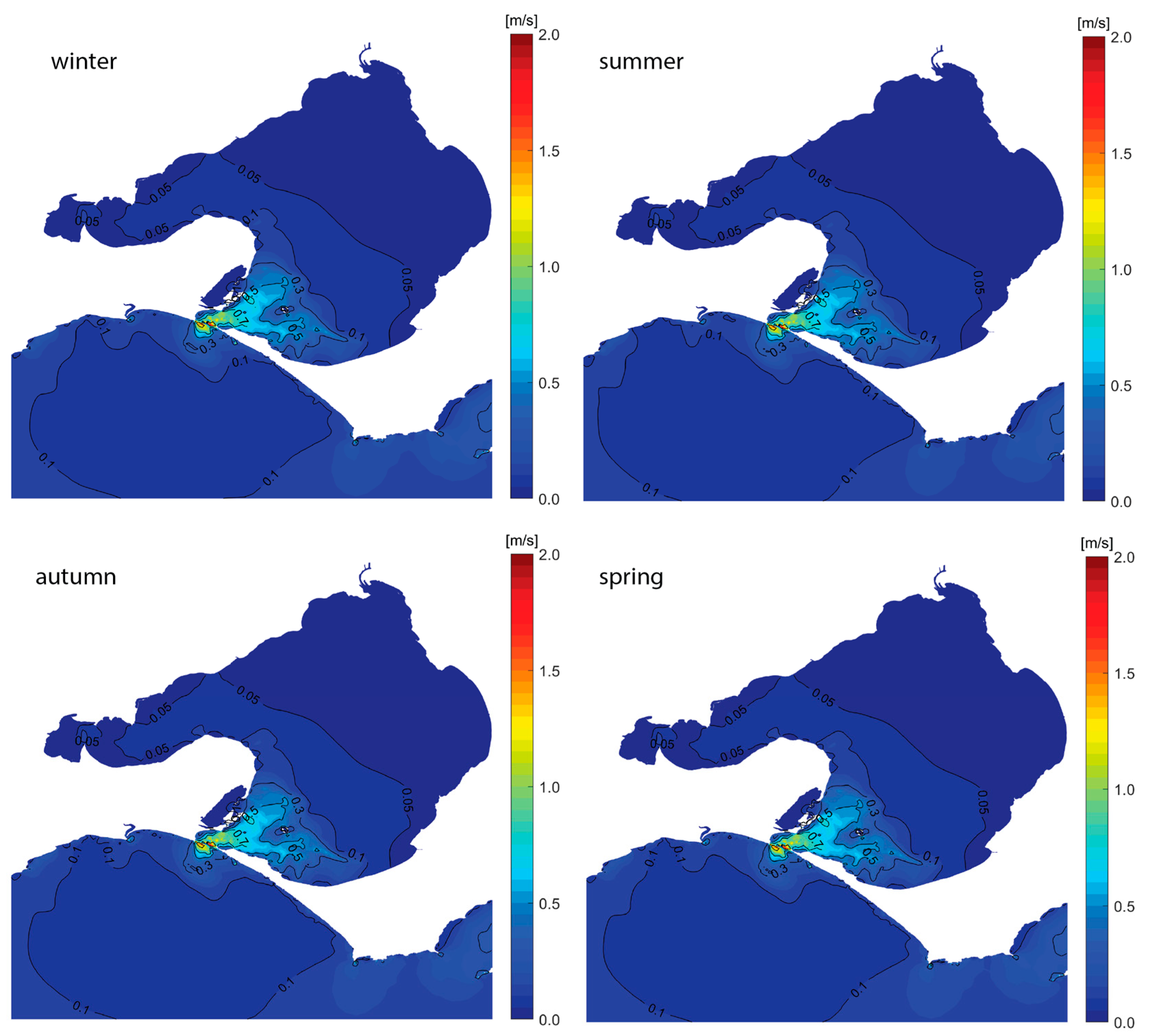
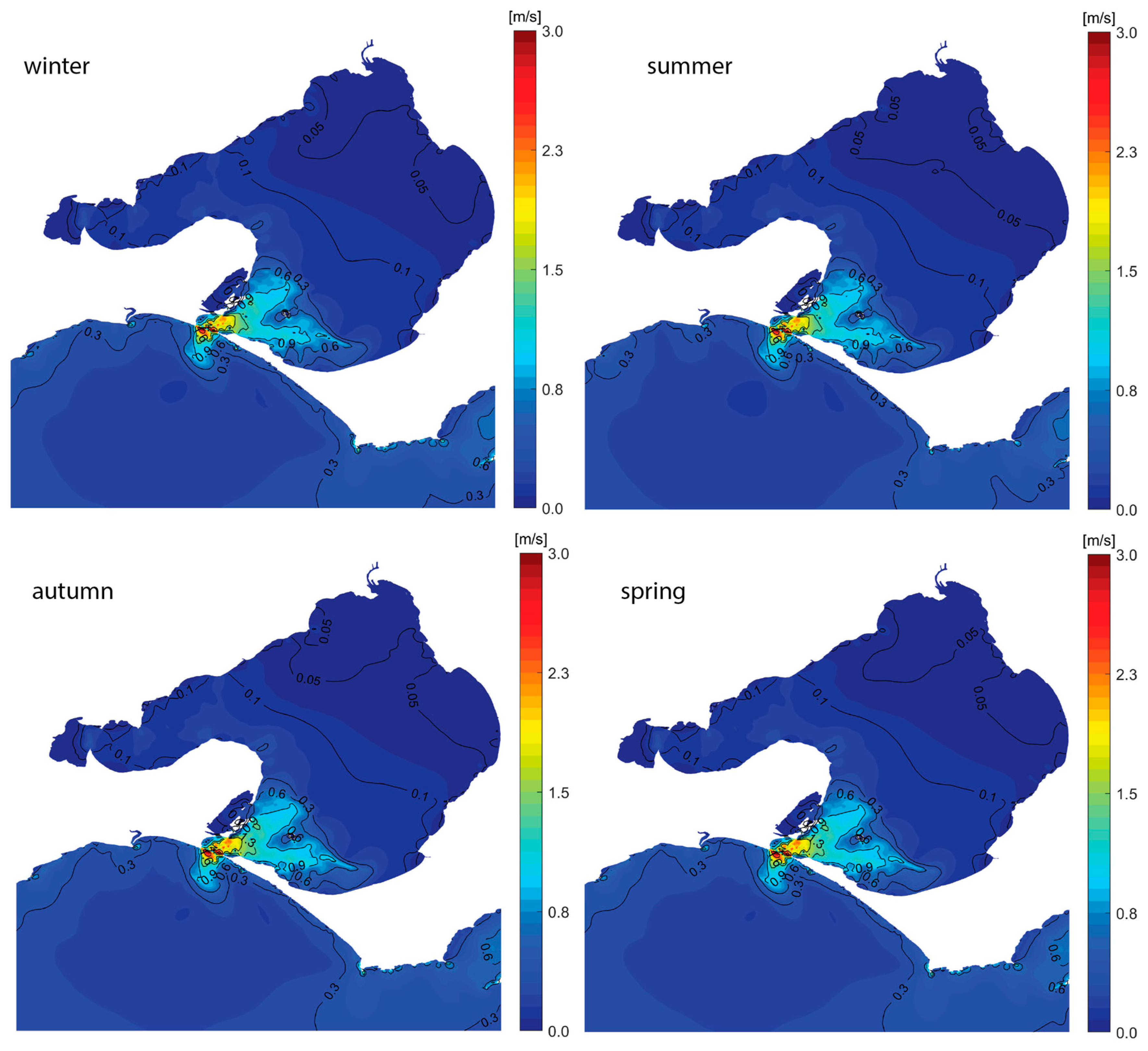
3.3. Seasonal Variations of Currents and Wind-Driven Circulations

Figure 14 shows the mean current speed for each season estimated over 27-year hindcasts. The strongest mean current speed up to 2 m/s is expected within PPH. The velocity gradually reduces when the current moves further into the South Channel (the main shipping channel) towards the northern portion of PPB. For the rest of PPB, the mean current is very weak, less than 0.1 m/s. It can also be seen that the mean current in PPB is not affected by seasonality. This indicates that astronomical tides are important for the currents in PPB. For high percentile levels, Figure 15 shows contours of the 99th percentile current magnitude across four seasons. Like the mean, there is no significant difference in the 99th percentile currents across different seasons. Compared to the mean value, there is a slight increase of 0.05 m/s in the 99th percentile current speed. With this high percentile level, a strong current of above 3 m/s is expected at the entrance of PPB.

It is noted that the present study does not estimate the return values of currents. This is because there is lack of a robust fitting method for the current field. Instead, we examined the influence of wind-driven currents in extreme conditions. This is an important aspect for PPB, which has not been studied up to now due to either lack of field data or computational resources. To do so, we used our validated numerical model to simulate extreme wind-driven currents with few case scenarios. Four different storms representing four different seasons were simulated including storms occurred in November 1994, February 2005, April 2009 and June 2014. These are the most extreme storms happening in PPB between 1990 and 2016. To illustrate typical circulation patterns during storm conditions, Appendix B (Figure A3) provides maps of wind-driven currents together with wind patterns modelled for the during the peak of the four storm events. A similar pattern of wind-driven circulations emerges across the four storms is that is there are two gyre systems forming in PPB lagoon. The major gyre is located in the central PPB while the minor gyre depends on the wind direction, but it is located near the coasts. These two gyres always rotate in an opposite orientation to each other. For February 2005 storm, the prevailing southerly wind is nearly perpendicular to the vertical axis of PPB. The wind-driven circulation inside PPB mainly rotates in a clockwise direction, creating the major gyre. The minor circulation system is located near the eastern coasts and rotates in a counterclockwise direction. For other three events, the peak occurred on 26 April 2009 at 03:00AM (autumn), on 24 June 2014 at 3:00AM (winter) and on 5 November 1994 at 4:00PM (spring), respectively, under a prevailing southwesterly wind. Of these events, the major gyre system rotates in a counterclockwise direction, while the minor gyre travels in a clockwise direction. The location of this minor gyre system in the case of the southwesterly wind is always the northeastern side of PPB—the direction towards which the wind blows. The presence of two gyre systems may be attributable to the weather system because PPB is located on the boundary between the subtropical system from the north and the westerly wind belt from the southern hemisphere (Cardno Lawson Treloar [6]). In terms of magnitude, strong wind-driven currents are mainly concentrated in shallow regions in the southern portion of PPB and around the Great Sands. In these shallow areas, it can also be seen that the wind direction also influences the wind-driven current magnitude. For instance, in the extreme event on 24 June 2014 at 03:00AM, the entrance of PPB receives strong southwesterly wind conditions, which travelled at a right angle to the entrance at about 210⁰. This wind direction induced a strong wind-driven current, up to 0.5 m/s, covering a large region from PPH to the Sand Islands. Similarly, when two gyres are created outside in Bass Strait, the rotational convention of these systems are the same as inside PPB.

4. Conclusions

This paper presents a comprehensive study dedicated to the Port Phillip Bay hydrodynamic climate with the aid of numerical modelling and field data. Both long-term and case scenario simulations were undertaken based on validated numerical models. The present study focused on three major aspects of hydrodynamics: water levels, waves and currents. The first two aspects focused on seasonal variations and extremes. Estimates of return periods were undertaken for water levels (storm tides) and SWHs. Case scenarios were also conducted to examine the wind-driven circulation over the study domain.

For sea levels, this study shows that the high percentile and extreme sea levels at many locations across PPB are nearly identical. This indicated that either the tidal elevation or the extreme level in PPB is almost the same. During extreme events, the highest storm tide level is found in the east coasts of PPB, in line with the wind patterns. For example, the frontal low weather system often forces the wind blowing from west to east. Through the 100-year return estimates, this study found that there is a reduction in extreme sea levels in the vicinity of PPH from the entrance to the Great Sand Islands. In this region, waves are attenuated due to friction and wave breaking. Such wave attenuation at the bay entrance often has a negative impact on (e.g., reducing) the extreme sea level.

For the wave field, the wave direction in PPB is strongly affected by the weather systems. During summer, wind blows from south to north and moves from north to south in winter, and the wave direction of propagation also follows this pattern. Unlike the inner PPB region, the wave direction in PPH area is dominated by swell propagation. The prevailing direction is about 210⁰ regardless of seasonality. After passing PPH, ocean waves get refracted towards the main tidal inlets and shipping channels. Estimates of 100-year return periods indicated that the significant wave height in PPB is bigger than 2 m, and the largest waves are found on the eastern coasts of PPB. Overall, the western coasts of PPB suffer fewer extreme waves than the eastern coasts. This study also found that the 100-year return SWH is similar to the maximum SWH found in the 27-year hindcast data. In the southern portion of PPB, this study found that ocean waves ocean waves passing the entrance of PPB penetrating further into the inlet. The evidence is shown in an estimate of the 90th percentile wave peak period of between 10 and 14 s covering a large area along the shipping channel and up to an area near West Channel Pile.

For currents, the current speed is only strong in the southern portion of PPB and PPH. It is very weak in the central and northern regions of PPB. At the 99th percentile level, the current speed at PPH exceeds 3 m/s. At both mean and high percentile levels, the current magnitude in PPB is not affected by seasonality. This indicated that astronomical tide is an important driver for flow movements within PPB. For wind-driven circulation, extreme wind conditions are expected to induce strong currents on shallow regions mainly located in the southern region of PPB. A wind-driven current of up to 0.5 m/s is found around the shallow areas near the Sand Islands. During extreme events, there are often two different gyre circulations induced by the weather systems inside PPB.

In conclusion, this study conducted a comprehensive investigation on hydrodynamic climatology of Port Phillip Bay, Australia based on both numerical modelling and field data available. Especially, this study conducted 27-year long-term hindcasts which have not been done in PPB so far. Furthermore, the coupled numerical modelling system used in this study was integrated with the advanced wave physics—the observation-based physical ST6 package with high resolution unstructured grid. However, it is noted that findings from this research are not exhaustive. For example, the influence of the propagation of astronomical tides alone on hydrodynamics (e.g., waves and surges) is subjected to a further study. This may require us to re-run 27-year hindcasts without tidal forcing. Further studies will also look at 3D effects on storm surges and compound flooding in coastal inundation. Due to lack of wave measurements inside PPB at the time of conducting this research, a further validation of the wave model is currently being undertaken with a new buoy system, which has been recently deployed in PPB.

References

1. Short, A.D. Beaches of the Victorian Coast and Port Phillip Bay; Coastal Studies Unit, Dept. of Geography, University of Sydney: Sydney, Australia; Surf Life Saving Australia: Sydney, Australia, 1996. [Google Scholar]
2. DELWP. Environmental Management Plan 2017–2027; Environment, Land, Water and Planning: Melbourne, Australia, 2017.
3. Bradford, S.; Siebinga, M. Communicating about dredging in a precious environment: Port of Melbourne Channel Deepeing Project. Terra Et Aqua 2009, 116, 12–20. Available online: https://www.iadc-dredging.com/wp-content/uploads/2017/02/article-communicating-about-dredging-in-a-precious-environment-port-of-melbourne-channel-deepening-project-116-2.pdf (accessed on 12 March 2020).
4. Provis, D.G.; Aijaz, S. Hydrodynamics of port Phillip Heads. In Proceedings of the 17th Australasian Coastal and Ocean Engineering Conference 2005 and the 10th Australasian Port and Harbour Conference 2005, COASTS and PORTS 2005, Adelaide, Australia, 20–23 September 2005; Robert, M., Walker, D., Eds.; Institution of Engineers, Australia: Barton, Australia, 2005; pp. 245–250, ISBN 978-1-62276-427-3. [Google Scholar]
5. Provis, D. Reflected waves in Port Phillip heads. In Proceedings of the Australian Coasts and Ports 2015 Conference, Auckland, New Zealand, 15–18 September 2015; pp. 739–744. [Google Scholar]
6. Treloar, C.L. Hydrodynamics and Coastal Processes; Maunsell Australia Pty Ltd.: Milton, Australia, 2007. [Google Scholar]
7. Lesser, G.; Turner, M.; Provis, D. Understanding the waves at Port Phillip Heads, Melbourne, Australia. In Proceedings of the 18th Australasian Coastal and Ocean Engineering Conference 2007 and the 11th Australasian Port and Harbour Conference 2007, COASTS and PORTS 2007, Melbourne, Australia, 18–20 July 2007. [Google Scholar] [CrossRef] [Green Version]
8. Hubbert, G.D.; McInnes, K.L. A storm surge inundation model for coastal planning and impact studies. J. Coast. Res. 1999, 15, 168–185. [Google Scholar]
9. McInnes, K.L.; Macadam, I.; Hubbert, G.D.; Abbs, D.J.; Bathols, J.A. Climate Change in Eastern Victoria. Stage 2 Report: The Effect of Climate Change on Storm Surges. 2005. Available online: http://www.cmar.csiro.au/e-print/open/mcinnes_2005b.pdf (accessed on 12 March 2020).
10. Mcinnes, K.L.; Macadam, I.; Hubbert, G.; O’Grady, J. An assessment of current and future vulnerability to coastal inundation due to sea-level extremes in Victoria, southeast Australia. Int. J. Climatol. 2013, 33, 33–47. [Google Scholar] [CrossRef]
11. McInnes, K.L.; Hubbert, G.D. Extreme Events and the Impact of Climate Change on Victoria Coastline. Report to EPA and Melbourne Water. 1996. Available online: http://www.cmar.csiro.au/e-print/open/mcinnes_1996a.pdf (accessed on 12 March 2020).
12. Rapizo, H.; Babanin, A.V.; Provis, D.; Rogers, W.E. Current-induced dissipation in spectral wave models. J. Geophys. Res. Ocean. 2017, 122, 2205–2225. [Google Scholar] [CrossRef]
13. Arns, A.; Wahl, T.; Wolff, C.; Vafeidis, A.T.; Haigh, I.D.; Woodworth, P.; Niehüser, S.; Jensen, J. Non-linear interaction modulates global extreme sea levels, coastal flood exposure, and impacts. Nat. Commun. 2020, 11, 1–9. [Google Scholar] [CrossRef] [Green Version]
14. McInnes, K.L.; O’Grady, J.G.; Hubbert, G.D. Modelling sea level extremes from storm surges and wave setup for climate change assessments in Southeastern Australia. J. Coast. Res. 2009, 1005–1009. [Google Scholar]
15. Tran, H.Q. Hydrodynamic Modelling of a Wave-Dominated Tidal Inlet System: Port Phillip Bay, Australia. 2020. Available online: http://minerva-access.unimelb.edu.au/handle/11343/247819 (accessed on 5 June 2021).
16. Cardno Lawson Treloar Hydrodynamic and Wave Model Calibration and Validation; Maunsell Australia Pty on behalf of Port of Melbourne Corporation: Melbourne, Australia, 2007.
17. Zhang, Y.J.; Ye, F.; Stanev, E.V.; Grashorn, S. Seamless cross-scale modeling with SCHISM. Ocean. Model. 2016, 102, 64–81. [Google Scholar] [CrossRef] [Green Version]
18. Zhang, Y.; Baptista, A.M. SELFE: A semi-implicit Eulerian–Lagrangian finite-element model for cross-scale ocean circulation. Ocean. Model. 2008, 21, 71–96. [Google Scholar] [CrossRef]
19. Bertin, X.; Bruneau, N.; Breilh, J.-F.; Fortunato, A.B.; Karpytchev, M. Importance of wave age and resonance in storm surges: The case Xynthia, Bay of Biscay. Ocean. Model. 2012, 42, 16–30. [Google Scholar] [CrossRef]
20. Ye, F. Simulating storm surge and compound flooding events with a creek-to-ocean model: Importance of baroclinic effects. Ocean Model. 2019, 145, 101526. [Google Scholar] [CrossRef]
21. Zhang, Y.J.; Ye, F.; Yu, H.; Sun, W.; Moghimi, S.; Myers, E.; Nunez, K.; Zhang, R.; Wang, H.; Roland, A.; et al. Simulating compound flooding events in a hurricane. Ocean. Dyn. 2020, 70, 621–640. [Google Scholar] [CrossRef]
22. Hsiao, S.-C.; Chen, H.; Chen, W.-B.; Chang, C.-H.; Lin, L.-Y. Quantifying the contribution of nonlinear interactions to storm tide simulations during a super typhoon event. Ocean. Eng. 2019, 194, 106661. [Google Scholar] [CrossRef]
23. Chen, W.-B.; Chen, H.; Hsiao, S.-C.; Chang, C.-H.; Lin, L.-Y. Wind forcing effect on hindcasting of typhoon-driven extreme waves. Ocean. Eng. 2019, 188, 106260. [Google Scholar] [CrossRef]
24. Guérin, T.; Bertin, X.; Coulombier, T.; de Bakker, A. Impacts of wave-induced circulation in the surf zone on wave setup. Ocean. Model. 2018, 123, 86–97. [Google Scholar] [CrossRef]
25. Umlauf, L.; Burchard, H. A generic length-scale equation for geophysical turbulence models. J. Mar. Res. 2003, 61, 235–265. [Google Scholar] [CrossRef]
26. Roland, A.; Zhang, Y.J.; Wang, H.V.; Meng, Y.; Teng, Y.C.; Maderich, V.; Brovchenko, I.; Dutour-Sikiric, M.; Zanke, U. A fully coupled 3D wave-current interaction model on unstructured grids. J. Geophys. Res. Ocean. 2012, 117, 1–19. [Google Scholar] [CrossRef] [Green Version]
27. Tolman, H.L. Effects of numerics on the physics in a third-generation wind-wave model. J. Phys. Oceanogr. 1992, 22, 1095–1111. [Google Scholar] [CrossRef] [Green Version]
28. Donelan, M.A.; Babanin, A.V.; Young, I.R.; Banner, M.L.; McCormick, C. Wave-follower field measurements of the wind-input spectral function. Part I: Measurements and calibrations. J. Atmos. Ocean. Technol. 2005, 22, 799–813. [Google Scholar] [CrossRef]
29. Donelan, M.A.; Babanin, A.V.; Young, I.R.; Banner, M.L. Wave-follower field measurements of the wind-input spectral function. Part II: Parameterization of the wind input. J. Phys. Oceanogr. 2006, 36, 1672–1689. [Google Scholar] [CrossRef]
30. Babanin, A.V.; Tsagareli, K.N.; Young, I.R.; Walker, D.J. Numerical Investigation of Spectral Evolution of Wind Waves. Part II: Dissipation Term and Evolution Tests. J. Phys. Oceanogr. 2010, 40, 667–683. [Google Scholar] [CrossRef]
31. Erick Rogers, W.; Babanin, A.V.; Wang, D.W. Observation-consistent input and whitecapping dissipation in a model for wind-generated surface waves: Description and simple calculations. J. Atmos. Ocean. Technol. 2012, 29, 1329–1346. [Google Scholar] [CrossRef]
32. Zieger, S.; Babanin, A.V.; Erick Rogers, W.; Young, I.R. Observation-based source terms in the third-generation wave model WAVEWATCH. Ocean. Model. 2015, 96, 2–25. [Google Scholar] [CrossRef] [Green Version]
33. Liu, Q.; Young, I.R.; Qiao, F.; Guan, C.; Zieger, S.; Babanin, A.V.; Romero, L.; Erick Rogers, W. Observation-based source terms in the third-generation wave model WAVEWATCH III: Updates and verification. J. Phys. Oceanogr. 2018, 489–517. [Google Scholar] [CrossRef]
34. Carrere, L.; Lyard, F.; Cancet, M.; Guillot, A. FES 2014, a new tidal model on the global ocean with enhanced accuracy in shallow seas and in the Arctic region. In Proceedings of the EGU General Assembly Conference Abstracts 2015, Vienna, Austria, 12–17 April 2015; p. 5481. [Google Scholar]
35. Saha, S.; Moorthi, S.; Pan, H.L.; Wu, X.; Wang, J.; Nadiga, S.; Tripp, P.; Kistler, R.; Woollen, J.; Behringer, D.; et al. The NCEP climate forecast system reanalysis. Bull. Am. Meteorol. Soc. 2010, 91, 1015–1057. [Google Scholar] [CrossRef]
36. Saha, S.; Moorthi, S.; Wu, X.; Wang, J.; Nadiga, S.; Tripp, P.; Behringer, D.; Hou, Y.T.; Chuang, H.Y.; Iredell, M.; et al. The NCEP climate forecast system version 2. J. Clim. 2014, 27, 2185–2208. [Google Scholar] [CrossRef]
37. Rascle, N.; Ardhuin, F. A global wave parameter database for geophysical applications. Part 2: Model validation with improved source term parameterization. Ocean. Model. 2013, 70, 174–188. [Google Scholar] [CrossRef] [Green Version]
38. Cazenave, A.; Remy, F.; Dominh, K.; Douville, H. Global ocean mass variation continental hydrology and the mass balance of Antarctica ice sheet at seasonal time scale. Geophys. Res. Letters 2000, 27, 3755–3758. [Google Scholar] [CrossRef]
39. DiLorenzo, J.L. The Overtide and Filtering Response of Small Inlet/Bay Systems. In Hydrodynamics and Sediment Dynamics of Tidal Inlets; Aubrey, D.G., Weishar, L., Eds.; Springer: New York, NY, USA, 1988; pp. 24–53. [Google Scholar]
40. Association of Bayside Municipalities. Port Phillip Bay Sea Level–Report 03. 2015. Available online: https://abm.org.au/wp-content/uploads/2018/12/ABM0004_ReportSeries_report_3.pdf (accessed on 12 March 2020).
41. Dunn, S.L.; Nielsen, P.; Madsen, P.A.; Evans, P. Wave Setup in River Entrances. Presented at the 27th International Conference on Coastal Engineering (ICCE), Sydney, Australia, 16–21 July 2000; pp. 3432–3445. [Google Scholar]
42. Hanslow, D.J.; Nielsen, P.; Hibbert, K. Wave Setup at River Entrances. Coast. Eng. 1996, 1997, 2244–2257. [Google Scholar] [CrossRef]
43. Young, I.R.; Zieger, S.; Babanin, A.V. Global trends in wind speed and wave height. Science 2011, 332, 451–455. [Google Scholar] [CrossRef]
44. Young, I.R.; Ribal, A. Multiplatform evaluation of global trends in wind speed and wave height. Science 2019, 364, 548–552. [Google Scholar] [CrossRef]
45. Vinoth, J.; Young, I.R. Global estimates of extreme wind speed and wave height. J. Clim. 2011, 24, 1647–1665. [Google Scholar] [CrossRef]
46. Meucci, A.; Young, I.R.; Breivik, Ø. Wind and wave extremes from atmosphere and wave model ensembles. J. Clim. 2018, 31, 8819–8842. [Google Scholar] [CrossRef]
47. Takbash, A.; Young, I.R.; Breivik, O. Global Wind Speed and Wave Height Extremes Derived from Long-duration Satellite Records. J. Clim. 2019, 32, 109–126. [Google Scholar] [CrossRef]
48. Coles, S. An Introduction to Statistical Modeling of Extreme Values; Springer: London, UK, 2001. [Google Scholar]
49. de Zea Bermudez, P.; Kotz, S. Parameter estimation of the generalized Pareto distribution-Part I. J. Stat. Plan. Inference 2010, 140, 1353–1373. [Google Scholar] [CrossRef]
50. de Zea Bermudez, P.; Kotz, S. Parameter estimation of the generalized Pareto distribution-Part II. J. Stat. Plan. Inference 2010, 140, 1374–1388. [Google Scholar] [CrossRef]
Figure 1. Location of study: (a) PPB location in map of Australia; (b) the overall bathymetry features of PPB with various observational stations used in the present study (c) a zoomed area showing the complexity of bathymetry within the southern portion of PPB including the entrance with various observational stations. At the entrance, there is a deep canyon up to 90 m depth at a narrow entrance where ocean waves often interact with a strong tidal current.
Jmse 09 00898 g001
Figure 2. Estimated maximum water levels (AHD) at different stations based on hourly data from tidal gauges.
Jmse 09 00898 g002
Figure 3. Measured wind data from 1998 to 2013 (mean speed, and direction) at the South Channel Island station during summer and winter months.
Jmse 09 00898 g003
Figure 4. Scatter plots compare the significant wave height and the mean wave direction (left panels) and the deep-averaged current speed and the direction (right panels) measured by bottom-mounted sensors (e.g., AWAC) within the entrance of PPB between 2006 and 2012 at NBCL (top panel), RBCL (middle panel) and ORBCL (bottom panel).
Jmse 09 00898 g004
Figure 5. Q-Q plots showing the relationship between ERA5 and measured mean wind speed (left) and CFSR and measured mean wind speed (right) at the South Channel Station for over 15-year period (1998–2013). The CFSR and ERA5 data were interpolated into the coordinate of the coordinate of the South Channel Station.
Jmse 09 00898 g005
Figure 6. Timeseries plots presenting several parameters obtained in the validation of ST6 physics in the WWM model for PPB: (a,d)—comparisons between model wind input and measured wind (speed, direction) at the South Channel Station in August 2003; (b,c)—comparisons between measured and modelled significant wave height at buoys near Rosebud; (e)—a comparison between modelled (mean) wave direction at one of the two wave buoys and field data. The WWM model performs well with both physical settings (ST4, ST6), but the modelled results with ST6 physics are better specifically in case of a high wind speed. It is noted that when there is a sudden change in the wind direction, both WWMIII with both ST4 and ST6 physics underestimated the SWH.
Jmse 09 00898 g006
Figure 7. Comparisons between the measured and field data obtained during calibration and validation. For SCHISM, plots for water level and depth-averaged velocity at ORBCL are shown in (A1,A2) and (B1,B2), respectively. For WWMIII, the SWH at the offshore buoy location is shown in (D1,D2). The SWH for the coupling model at ORBCL is shown in (C1,C2).
Jmse 09 00898 g007
Figure 8. Seasonal variations in sea levels with respect to the mean value, 90th and 99th percentiles. The MSL in PPB shows a strong influence of seasonality.
Jmse 09 00898 g008
Figure 9. A map showing the 100-year return storm tide levels based on 27-year hindcast using POT method.
Jmse 09 00898 g009
Figure 10. Spatial distribution of mean wave direction (Dir), wave peak period (Tp) and SWH (Hs) for the four seasons. For the ease of interpretation, the same color-scale is kept for both mean value in this figure and the higher percentiles and extremes in Figure 11.
Jmse 09 00898 g010
Figure 11. Maps of spatial and seasonal variations in SWH estimated for the 90th and 99th percentiles and maximum values over 27-years hindcasts.
Jmse 09 00898 g011
Figure 12. The 90th percentile wave peak period during summer and winter estimated from 27-year hindcasts.
Jmse 09 00898 g012
Figure 13. Estimates of the 100-year return SWHs based on different threshold levels: the 90th (a), 95th (b), 99th (c) and 99.5th (d) percentiles using POT approach.
Jmse 09 00898 g013
Figure 14. Seasonal variations in the mean current velocity. The mean magnitude can reach 2 m/s in the vicinity of PPH. After passing the southern region, the current speed is very weak.
Jmse 09 00898 g014
Figure 15. Maps showing the 99th percentile current speed. The magnitude goes beyond 3 m/s in the vicinity of PPH. However, in the inner regions of PPB, the current speed is weak with the magnitude of about 0.1 m/s.
Jmse 09 00898 g015