Assessing Extreme Environmental Loads on Offshore Structures in the North Sea from High-Resolution Ocean Currents, Waves and Wind Forecasting

Abstract

The fast development of the offshore energy industry becomes an essential component of resilient economies in most of the countries around the North Sea, addressing an increasing demand for cost-efficient and environmentally safe energy sources. Offshore wind farms are planned to be installed further away from the coasts to ensure stronger and more stable wind resources in this region. Oil and gas extraction infrastructures are also planned to move into deeper areas of the continental shelf and continental shelf slopes to explore new fields. These deeper areas of the ocean are characterised by harsh environmental conditions: stronger winds, larger waves and strong shelf slope currents, inducing considerably larger loads on offshore structures. This study brings together operational physical oceanography and the mathematics of fluid-structure interactions to estimate the likelihood of extreme environmental loads on offshore structures in the North Sea. We use the state-of-the-art Met Office high resolution ocean forecasting system, which provides high-frequency data on ocean and tidal currents, wave heights and periods and winds at a ~7 km horizontal resolution grid, spanning the North–West European Shelf. The Morison equation framework is used to calculate environmental loads on various types of offshore structures that are typically employed by the offshore industries in the North Sea. We use hourly data for a 2-year period to analyse the spatio-temporal variability of mean and extreme hydrodynamic loads and derive the relative contributions of currents, waves and winds in the region. The results indicate that waves dominate extreme hydrodynamic forces on the shallow shelf, whereas the current contribution is important at the shelf break and in the English Channel.

1. Introduction

Engineering analysis of floating or fixed offshore structures requires the assessment of environmental loads from winds, waves, and currents [1,2,3,4,5]. In the fast-growing wind energy market of the North Sea, offshore wind farms are planned to be installed further away from the coast to ensure access to a stronger and more stable wind field, while avoiding impacts on the local shoreline environment and the viewshed from the shores [6,7]. Oil and gas extraction structures are also planned to be relocated in the deeper areas to operate in new fields [8,9]. These emerging industrial opportunities imply new challenges, as going further offshore requires the construction of stronger and more complex foundations with higher investment and maintenance costs [5]. Ocean areas of deeper continental shelves and of continental shelf slope areas in the North Sea present higher risks due to considerably larger loads on offshore structures caused by stronger winds, larger waves and strong slope currents—these have important implications for operational safety and should be taken into account in the design of the offshore structures and in planning their exploitation [10]. The highest wave conditions in the global ocean are encountered in the northeast Atlantic [11], strongly affecting the continental slope around the northern North Sea in particular [12]. This region is also affected by the Northeast Atlantic slope current—a year-round strong current flowing northwards along the steep continental slope around the Northwest European Shelf Seas with maximum values obtained in the Faeroe–Shetland Channel [13]. The North Sea is also a tidally dominated region, with tidal currents exceeding 1 m/s in the southern parts and the English Channel [14].

Accessing pertinent data relevant to a specific at-sea area of operation is less straightforward for the engineer or mathematician using analyses based on wave radiation influences and diffraction, or inertia-drag prediction techniques. The observation and simulation of realistic ocean currents is the specialty of physical oceanographers and marine weather forecasters. Hence, an integrated approach requires the synergistic and collaborative effort between physical oceanography/weather marine forecasting and offshore engineering, in concert with the industry concerned with marine advice and safety.

In the past, impacts of ocean currents and waves on offshore structures were often oversimplified. More recently, new methodologies are applied in offshore engineering to take into account the complexity of the wave field around offshore structures, such as copula-based models which use the joint distribution function of the significant wave height and spectral peak period to obtain the probability of failure of scour protections for wind turbine foundations [15]. It is also very important to recognise the various sources of current variability throughout the water column involving a large range of spatial and temporal scales, such as surface and bottom frictional Ekman layers, strong baroclinic jets which can peak at mid-depth, and intensified flows at depth (e.g., turbidity currents) associated with local bathymetric features, tidal currents, and near-surface inertial currents (in response to storm forcing) which can dominate tidal currents for days. Hence, it is necessary to develop a better representation of the vertical structure and temporal variation of ocean currents to estimate the wave-current load variability on offshore structures more accurately. Furthermore, tidal forcing is often the dominant contributor to the ocean forcing in coastal and shelf seas such as the North Sea, exceeding large scale geostrophic barotropic/baroclinic currents by an order of magnitude.

The use of only in situ current measurements in determining loads on offshore structures is problematic, since although these may provide high-frequency current data, they may not be representative of the varying regime of the ocean currents in the area of interest. Sometimes the costs, as well as the long waiting period, are prohibitive for the currents’ observations to be used in the structure design, as at least 12 months of measurements are needed to perform a valid statistical analysis of extremes. Satellite-derived sources, while providing a synoptic picture of the surface current regime, can neither provide information about the 3-D current structure varying with depth, nor represent high-frequency variability, which are both crucial for estimating the combined wave–current loads on offshore structures.

Ocean hindcasts using air-sea forcing from atmospheric re-analyses, and specifically, operational ocean nowcasts and forecasts based on the assimilation of all available ocean observations, can provide detailed information on the 3-D structure of currents in an area of operations. From the 1990s, the offshore oil industry started to use 3-D numerical models to estimate impacts of environmental conditions on offshore structures for both design and operational purposes. The North European Storm Study (NESS), an oil industry and government agency sponsored a modelling study of wind, wave, and current conditions on the North European Continental Shelf [16]. The North-West Approaches Group (NWAG), an oil industry consortium, has invested extensively into measuring the current regime west of Shetland and developing a 3-D ocean model, producing more reliable current information for design input and operations support in that region [17]. The University of Colorado, in one of the first operational oceanography applications in the offshore oil industry, used operational nowcast/forecast numerical models to predict current regimes associated with the Loop Current and its Eddies in the Gulf of Mexico and the Caribbean [18]. In the past, ocean data quantity and quality were insufficient for model initialisation, boundary conditions and, importantly, validation. However, over the last 10 years, together with the increasing spatial resolution of atmospheric and ocean models, the emergence of new high-quality data sources (e.g., new and higher resolution satellite-derived products, ARGO floats, gliders) led to a large increase in the number of observations, allowing for better model initialisation/validation. The assimilation of this high quantity/quality observational information in the operational modelling systems has also significantly improved the accuracy of hindcasts, nowcasts and forecasts. Currently, there are strong requirements from the offshore industries for high-resolution ocean forecasting to evaluate the impact of extreme ocean conditions on offshore structures. The design constraints for survivability of the offshore structures needs information on extreme ocean and weather conditions for input into design criteria, whereas high-frequency forecasts enable the identification of suitable operational windows.

This paper brings together expertise and methods from the operational physical oceanography, marine weather forecasting and the mathematics and fluid structure interaction to address the likely extreme loads on a selection of offshore structures typically employed in the North Sea. We use the Met Office high resolution coupled ocean–wave forecasting system, offering high frequency environmental data output, including ocean and tidal currents, waves and winds on a ~7 km resolution grid covering the North-West European Shelf. The Morison equation [19] is used here to calculate hydrodynamic loads on various types of offshore structures, including jackets and fixed/floating monopiles of different dimensions typically employed by the offshore industries in the North Sea. We assess the spatiotemporal variability of mean and extreme hydrodynamic loads on the various types of offshore structures. We also focus on the relative contributions of currents and waves on the total hydrodynamic loads and their spatial variations in the North Sea. Finally, we assess the impact of spatial resolution of ocean circulation and wave models on the hydrodynamic load calculations. Our ultimate goal is to better assess environmental loads on offshore structures based on high-quality met-ocean data from a state-of-the-art forecasting system. The improvement of loads quantification may have a direct impact on the optimization of offshore structures for both design and operational purposes, including a better assessment of dynamic scour protections of structure foundations, maintenance, and various operation activities.

2. Methods and Data

2.1. Methodology

We use Morison equation (hereon ME) [19] to estimate the hydrodynamic force on offshores structures. ME is essentially composed of Froude–Krylov and accelerated fluid influences within the inertia terms and the non-negligible boundary layer influence captured in the drag term (for details, see [19]). The inertia-drag dependent total hydrodynamic force (wave and current combined) on a horizontal cross-section of a thickness $dz$ of a “fixed” cylindrical structure due to ocean waves and spatially and temporarily varying currents is expressed in the form:

$$\delta F=\left[\rho A{C}_M\dot{u}\pm \rho A\left(1-C_M\right)\left\{\frac{\partial U}{\partial t}+\left(u \pm U\right)\frac{\partial U}{\partial x}\right\}+\frac{1}{2} \rho D{C}_D \left(u\pm U\right)\left|\left(u\pm U\right)\right|\right] dz$$

(1)

for which $u$, $\dot{u}$ are the wave-induced velocity and acceleration in the structure location at given time $t$, respectively, $U=U\left(x, z,t\right)$ is the current velocity ($\pm$ sign dictates whether the current is reinforcing or opposing the wave propagation), $x$ is the coordinate in the direction of wave propagation, with $x$ = 0 aligned with the vertical axis of the cylindrical structure, $z$ is the vertical co-ordinate, $C_M$ and $C_D$ are inertia and drag coefficients, respectively, $\rho$ is the seawater density, $D$ is the cylinder diameter, and $A=\pi ·D^2/4$ is the cross-section area. The Morison equation is valid only for slender objects, so that the diameter of the vertical cylinder $D$ must be significantly smaller than the wavelength λ (typically $D/\lambda <0.2$).

Here, we neglect the acceleration and the spatial variation in the ambient water flow near the cylinder, assuming undisturbed flow in the immediate vicinity of the cylinder at any given time. Following linear wave theory, for waves propagating in the x-direction the wave-induced velocity and acceleration at location $x=0$ (aligned with the vertical axis of the structure), are given by:

$$u\left(x=0,z,t\right)=\omega a\frac{cosh\left(k\left(h+z\right)\right)}{sinh\left(kh\right)}sin\left(\omega t\right)$$

(2)

$$\dot{u}\left(x=0,z,t\right)={\omega }^{2}a\frac{cosh\left(k\left(h+z\right)\right)}{sinh\left(kh\right)}cos\left(\omega t\right)$$

(3)

where $\omega$ is wave angular velocity, $a$ is the maximum wave amplitude, $k$ is the wave number, $h$ is water depth, and $t$ is time. Due to the fact that the drag term depends on the velocity, while the inertia term depends on the acceleration, the occurrence of the maximum drag force and the maximum inertia force are separated by a phase shift of 90°. The maximum force is then calculated as the maximum value over a wave period.

$C_M$ and $C_D$ are both functions of Keulegan–Carpenter number [20], a measure for the ratio between the wave height and the cylinder diameter, and Reynolds number, in addition to an outer surface condition expressed in terms of the degree of roughness [2,21]. It should be noted that $C_D$ increases with increasing roughness, whereas $C_M$ decreases with increasing roughness. $C_M$ also decreases with increasing cylinder diameter to wavelength ratio ($D/\lambda$) [3]. Here, for our demonstration case study, we fixed these coefficients at typical values of $C_{M }$= 1.4 and $C_D$ = 0.7, without either further justification or variation.

To obtain the total hydrodynamic load on the structure $F_{tot}$ we integrate (1) by $dz$ for the whole height of the cylindrical structure. Since the structure displacement is neglected, we can drop the dependency on the coordinate $x$:

$$F_{tot}\left(t\right)=\underset{0}{\overset{Z}{{\displaystyle \int }}}dF\left(z,t\right) dz$$

(4)

Here, $z$ is the height of the cylindrical structure. The integration of (4) is done numerically using the Simpson’s method.

In order to calculate the wind load on the wind turbine tower, we make the approximation that it is a cylinder of constant diameter (although, in general, the diameter of the tower decreases as we get closer to the rotor). Wind forces on offshore structures are caused by complex fluid-dynamics and are generally difficult to calculate with high accuracy. Here, the wind drag force (per unit length) for a cylindrical pile at height $z$ is estimated by the parameterization [4]:

$$F_W\left(z\right)=\frac{1}{2}{\rho }_a C_w D V{\left(z\right)}^2$$

(5)

where ${\rho }_a$ is the mass density of air (~1.25 kg m⁻³), $D$ is the cylinder diameter, $C_w$ is the wind pressure coefficient, and $V\left(z\right)$ is the wind speed at height $z$. $C_w$ depends on the Reynolds number and is determined under controlled stationary wind flow conditions in a wind tunnel. For a cylindrical tube, a typical value of 0.7 is used in this study.

2.2. Data and Input Variables

We use high-resolution wave, ocean current and wind operational data over a 2-year period, from July 2014 to June 2016, provided by the Met Office. Surface currents (eastward and northward velocity components) are obtained from the Atlantic Margin Model (AMM7) [22], based on the Met Office Forecasting Ocean Assimilation Model (FOAM) [23,24] with the Nucleus for European Modelling of the Ocean (NEMO) model [25] as its hydrodynamic core [26], including tidal currents. Model spans the Northwest European continental Shelf (NWS) regional seas with a 7-km mesh and output frequency of 1 h. Significant wave height (SWH), wave peak frequency, and wave direction are obtained from the Wavewatch III model [27], gridded on the AMM7 grid with an hourly output frequency. A lower resolution Met Office wave dataset covering the whole North Atlantic at ~25 km resolution over the same period (July 2014 to June 2016) is also used to assess the impact of wave model spatial resolution on force calculations. Winds (eastward and northward wind speed components) at 10 m above sea level were also available on the AMM7 grid, with an hourly output frequency. More details about the AMM7 model configuration as well as model validation can be found in [22].

In addition, a global ocean model hindcast at 1/4° (ORCA025) and 1/12° resolution (ORCA12), developed and run at the National Oceanography Centre Southampton (NOCS), also based on the NEMO ocean model [25], is used here to compare with Met Office FOAM operational model in terms of ocean current spatio-temporal variability, and to assess the impact of model spatial resolution on the calculation of ocean current loads.

Concerning input variables for wave load calculations, we use the wave peak frequency $f_p$ from the Wavewatch III model to calculate angular peak frequency as $\omega =2\pi f_p$ and significant wave height ($SWH$) to obtain maximum wave amplitude as $a=1.8·SWH$.

We determine the wind speed profile by using a 1/7th power law; an empirical law tested with observations and widely used for estimation of wind power potential [28]:

$$V_z=V_{10}{\left(\frac{z}{10m}\right)}^{1/7}$$

(6)

where $V_z$ is the wind speed at elevation of $z$ m above sea level, $V_{10}$ is the wind speed at 10 m above sea level, and 10 m is the reference height.

Met Office wind data used here are provided for 10 m height; therefore, Equation (5) is used to evaluate the full wind speed profile in the 100 m layer above sea level. The above equation gives the mean wind component (hourly mean in our case). In order to determine the peak gust wind speed, we need to multiply mean wind speed by the so-called gust factor. For hourly mean wind and for offshore areas (>20 km offshore), the gust factor is ~1.3 [29]. Variation of the gust factor along the column height is considered negligible.

2.3. Offshore Structures: Demonstration Cases

ME can be applied to tubular (cylindrical) columns of varying diameters that represent various types of offshore structures typically used in the offshore oil and gas and offshore wind industries in the North Sea—namely fixed jackets, fixed monopiles, and floating (spar type) monopiles [30]. Calculations involve the integrated (along the whole tubular column height) combined hydrodynamic (wave/current) force for the submerged part of the column (fixed/floating monopiles and jacket legs) and the integrated wind (drag) force on the above sea level part of the column (fixed/floating monopiles). Details for the three general demonstration cases considered here are provided below:

(1)

Fixed jackets: these structures are commonly used for oil and gas extraction and to support wind turbines. Here, we consider depths varying from 5 m up to 500 m, although typical deployment depths are below 100 m in the North Sea. Two cases of tubular cylinder diameter ($D$) for the jacket legs are considered in this study: (a) $D$ = 1 m, and (b) $D$ = 2 m. The calculations involve only the submerged column height where the combined hydrodynamic (wave plus current) force is calculated.

(2)

Fixed monopiles: these structures are typically used to support wind turbines in the North Sea. A total depth up to 100 m is considered for the sub-merged part of the monopile. For the non-submerged column (above-sea level), a height of 100 m is considered. A typical diameter of 5 m is considered for a tubular cylinder for both the submerged and above-sea level parts of the monopile. The calculations involve the combined hydrodynamic (wave + current) force (submerged column) and the wind drag force (above sea level column).

(3)

Floating (spar type) monopiles: these structures are recently used to support wind turbines in the North Sea. Here, we consider a total depth from 100 m up to 1000 m. For the submerged part of the monopile a fixed height of 100 m with a diameter of 10 m is considered. For the above-sea level part of the monopile, a height of 100 m and a diameter of 5 m are used. The calculations involve the combined hydrodynamic (wave + current) force (submerged column) and the wind drag force (above-sea level column).

3. Results and Discussion

Here, we are using a case study of particular interest for the offshore oil and gas and offshore wind industries, the North Sea, to estimate the spatiotemporal variability of hydrodynamic loads from waves and currents modelled through the ME for the three types of offshore structures, as detailed above.

Although we focus on the North Sea, spatial maps of mean and maximum loads shown here are extended to cover the whole NW European Shelf to reveal load variability and extremes further away from the shelf in areas currently explored by the offshore energy industries for potential future exploitation of resources.

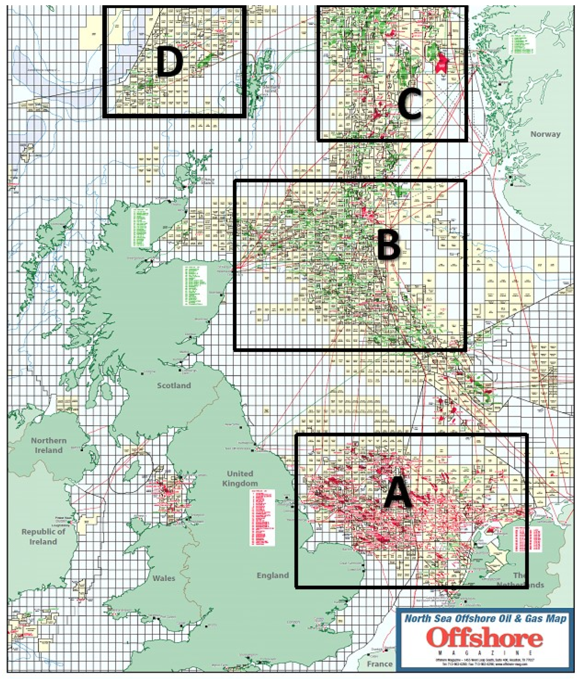
We perform a statistical analysis of mean and extreme loads focusing on 4 sub-areas of high offshore oil-gas and offshore wind energy production and/or production potential in the North Sea (see Figure 1), namely:

• Area A: Southern North Sea (offshore area roughly between Central/North England and Netherlands, average depth ~30 m), mainly offshore gas and wind energy production.
• Area B: Northern North Sea (roughly between Scotland and Norway, average depth ~90 m), mainly offshore oil production, new floating wind farms.
• Area C: Along the north Norwegian Shelf (average depth ~200 m), mainly offshore oil production.
• Area D: North Sea Slope Current area (average depth ~350 m), oil production with new exploitation licenses.

3.1. Hydrodynamic (Wave/Current) Force

Hydrodynamic load calculations are highly sensitive to the choice of the structure dimensions, i.e., monopiles and jacket legs of different diameter ($D$) and height. Since the inertia term in the Equation (1) depends on $D^2$ and the drag term depends linearly on $D$, the width of the structure is more important for wave loads, since they strongly decrease with depth, whereas the structure height is more important for current loads, which typically affect the whole water column. For fixed structures (monopiles and jackets), the ocean current contribution to the total hydrodynamic load (integrated over the whole tubular structure height) increases with depth, as current velocities remain relatively high in the deeper areas, whereas wave-induced velocities are considerably reduced. Consequently, there is a very large range in the calculated hydrodynamic loads due to their high sensitivity on the different dimensions/types of structures. Furthermore, we need to note that we only focus here on the quantification of the integrated force on tubular parts of the various types of structures, without assessing the level of significance for each type of structure, i.e., the same hydrodynamic load can have different significance between a moored floating structure and a seabed-mounted structure.

We first present analyses of the hydrodynamics forces associated with waves and currents, assessed spatially and temporally, for demonstration cases 1, 2 and 3.

3.1.1. Spatial Variability

Spatial variability of hydrodynamic (wave/current) forces (integrated along the whole height of a pile) are presented here by spatial maps of temporal mean and maximum values (in Newtons) over the 2-year period considered here (July 2014–June 2016) and for the 3 demonstration cases described above.

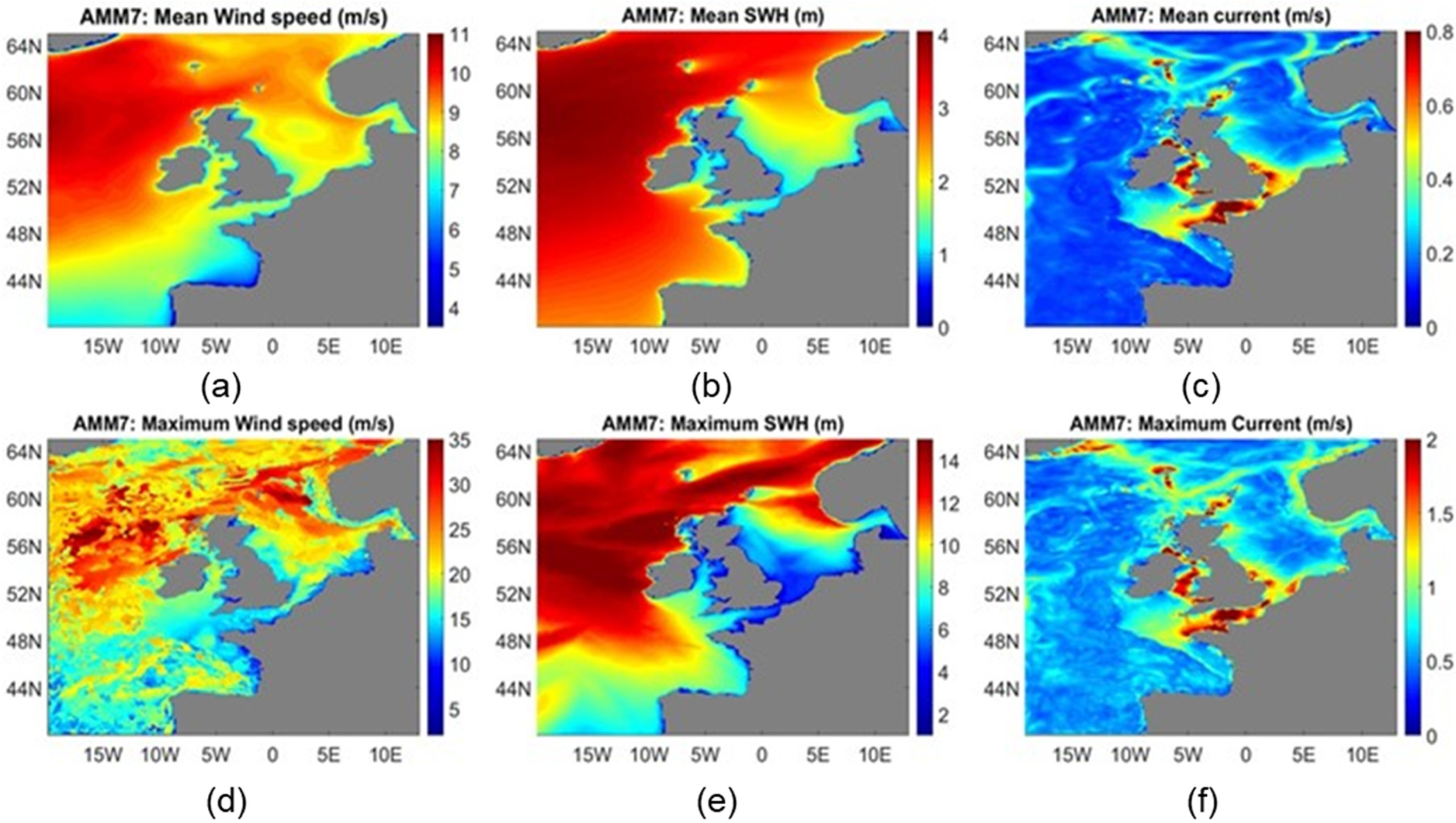
Figure 2 shows spatial maps of temporal mean and maximum values of wind speed, significant wave height, and current velocity from the Met Office AMM7 dataset. As expected, wave amplitude is highly correlated with wind speed with maximum SWH values located along the north-eastward pathway of storms in the North Atlantic. Maximum $SHW$ exceeds 15 m in the slope area of the northern North Sea, whereas maximum values are much lower in the southern North Sea Shelf and Irish Seas (<6 m). There is a strong north-eastward gradient of increasing $SHW$, from the UK east coast to the Norwegian shelf.

Eddy dynamics, small-scale current structure high-frequency features and tidal currents in particular, are readily identifiable in the simulated current velocity field. In contrast with the wave field the current velocity spatial pattern is not correlated with the wind, as the current field in this area is mainly dominated by tidal and baroclinic/slope currents. Maximum tidal current velocities exceed 1.5 m/s in the English Channel and Irish Sea, whereas relatively large maximum values of order 1 m/s are encountered in the northern slope area and along the Norwegian coast (Norwegian Coastal current).

Case 1

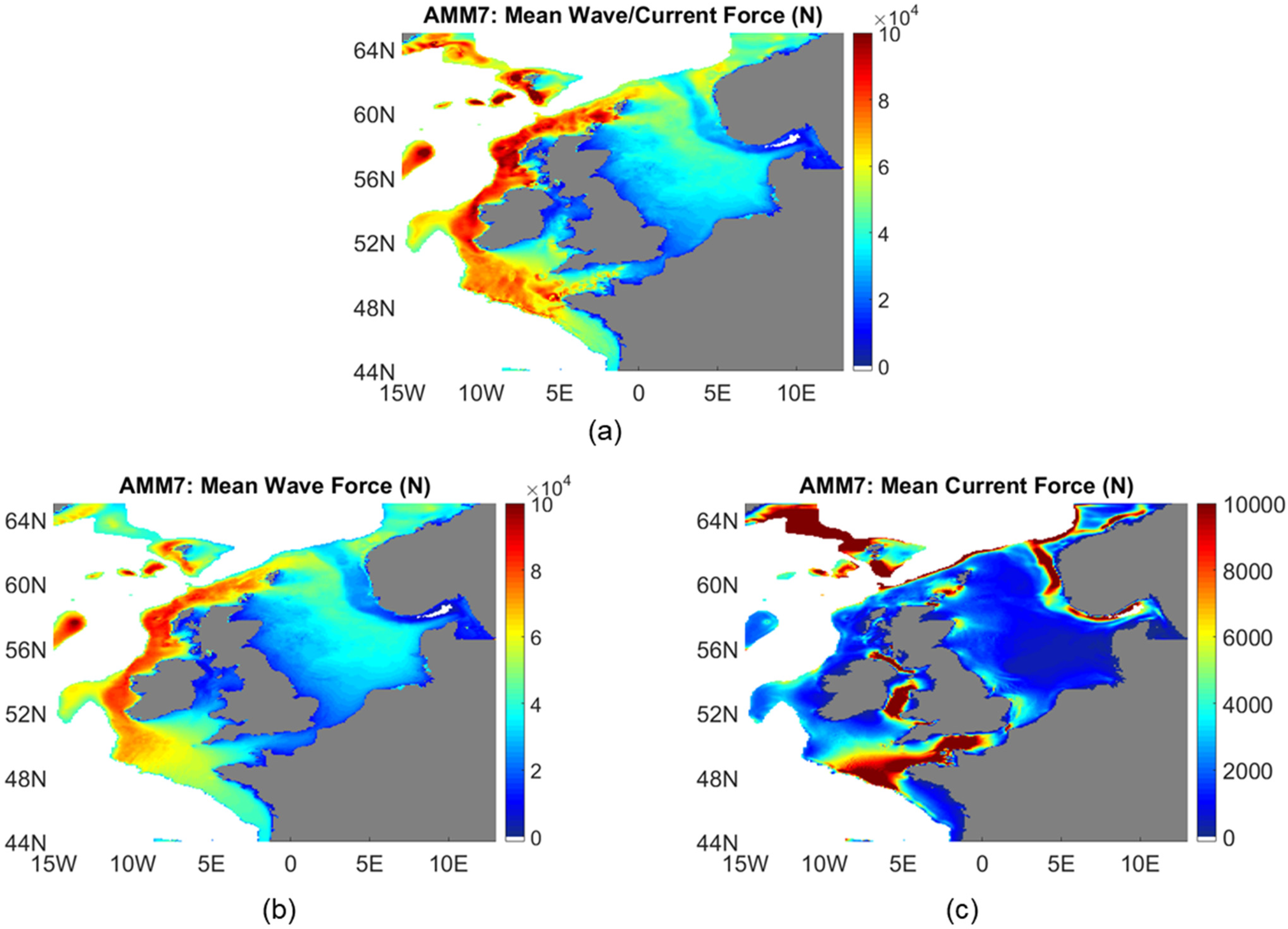
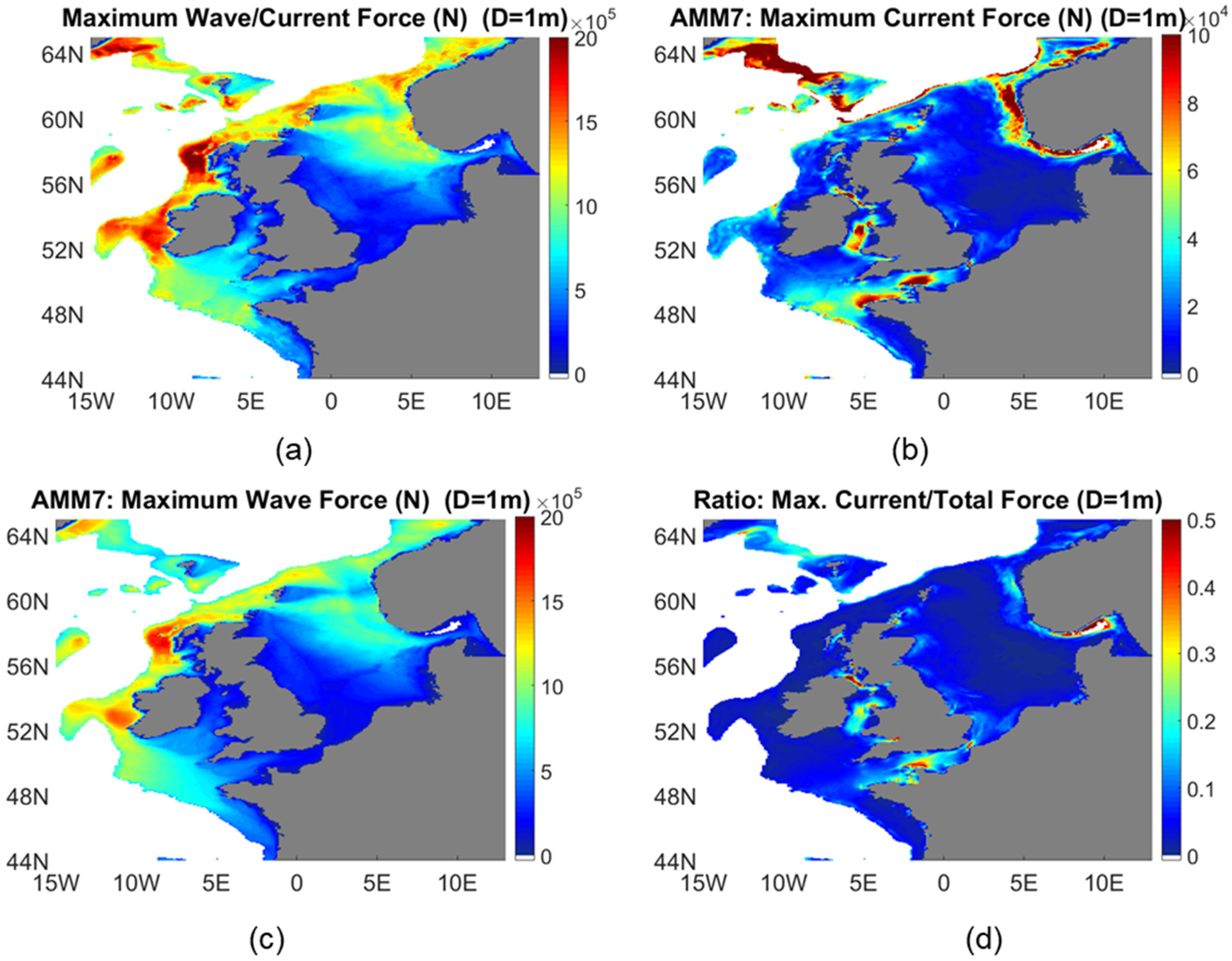
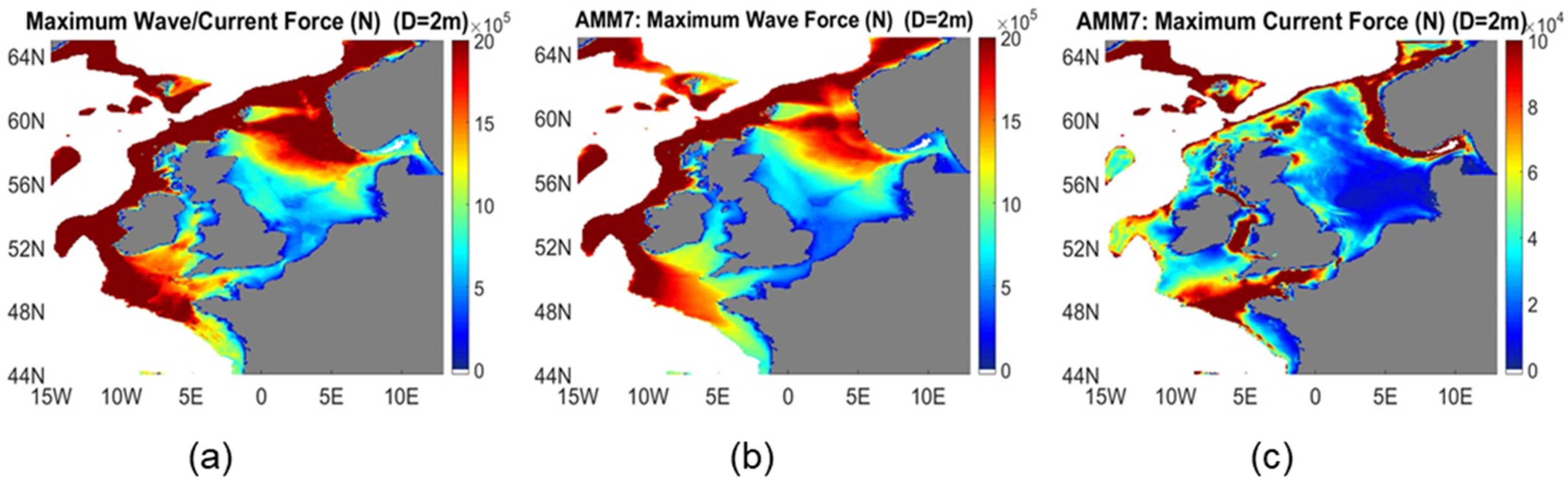
Figure 3 and Figure 4 show spatial maps of temporal mean and maximum values respectively of wave/current force, wave only force, and current only force on a jacket leg of diameter D = 1 m. As expected, current and wave forces have very different spatial patterns reflecting the large differences between the current and wave field spatial patterns described above. One exception is the slope area of the North Sea, where increased values of both wave amplitude and current velocity are obtained resulting in the strongest combined wave/current loads over the whole domain with the mean force reaching ~10⁵ N. The largest contributor to the mean force over the 2-year period is the wave force, which largely dominates spatial variability, except for the English Channel and Irish Sea, where tidal currents result in large current force contribution.

Due to the non-linearity of inertia and drag components in Morison equation (in terms of wave induced velocity and current velocity, respectively), maximum (extreme) wave/current force is at least an order of magnitude larger than the mean force throughout the domain over the 2-year period considered here (Figure 4). Maximum (extreme) force exceeds 10⁶ N in the slope area (up to 2 × 10⁶ N at the north-western part of the slope) over the 2-year period. However, maxima of the two components are not overlapping on the slope area. Current force maximum is located in deeper regions within the slope area (>400 m depth) whereas maximum wave force is encountered in more shallow water (200–400 m). On the shelf (depth < 200 m) maximum total force is typically much lower than in the slope area (~2–5 × 10⁵ N) with the exception of the north-eastern part of shelf (~10⁶ N) where storms typically enter the North Sea, resulting in higher wave amplitudes. As for the mean force wave, contribution to the maximum force is dominant throughout most of the region. The area-averaged ratio of current to total (wave/current) force is ~6%. Relatively large current contributions (up to 50%) are observed in the English Channel, Irish Sea and the Norwegian Coastal Current.

The increase of pile diameter from 1 m to 2 m results in approximately 2 times larger maximum current force component and 4 times larger maximum wave force component on the jacket leg (Figure 5). Extreme force over the 2-year period exceeds 2 × 10⁶ N in the whole slope area and north-eastern part of the North Sea shelf with the maximum over the whole area reaching 10⁷ N in the north-western part of the slope. The area-averaged ratio of current to total (wave/current) force slightly increases from ~5 % to ~6%, as the inertia term becomes increasingly more important with pile diameter increase.

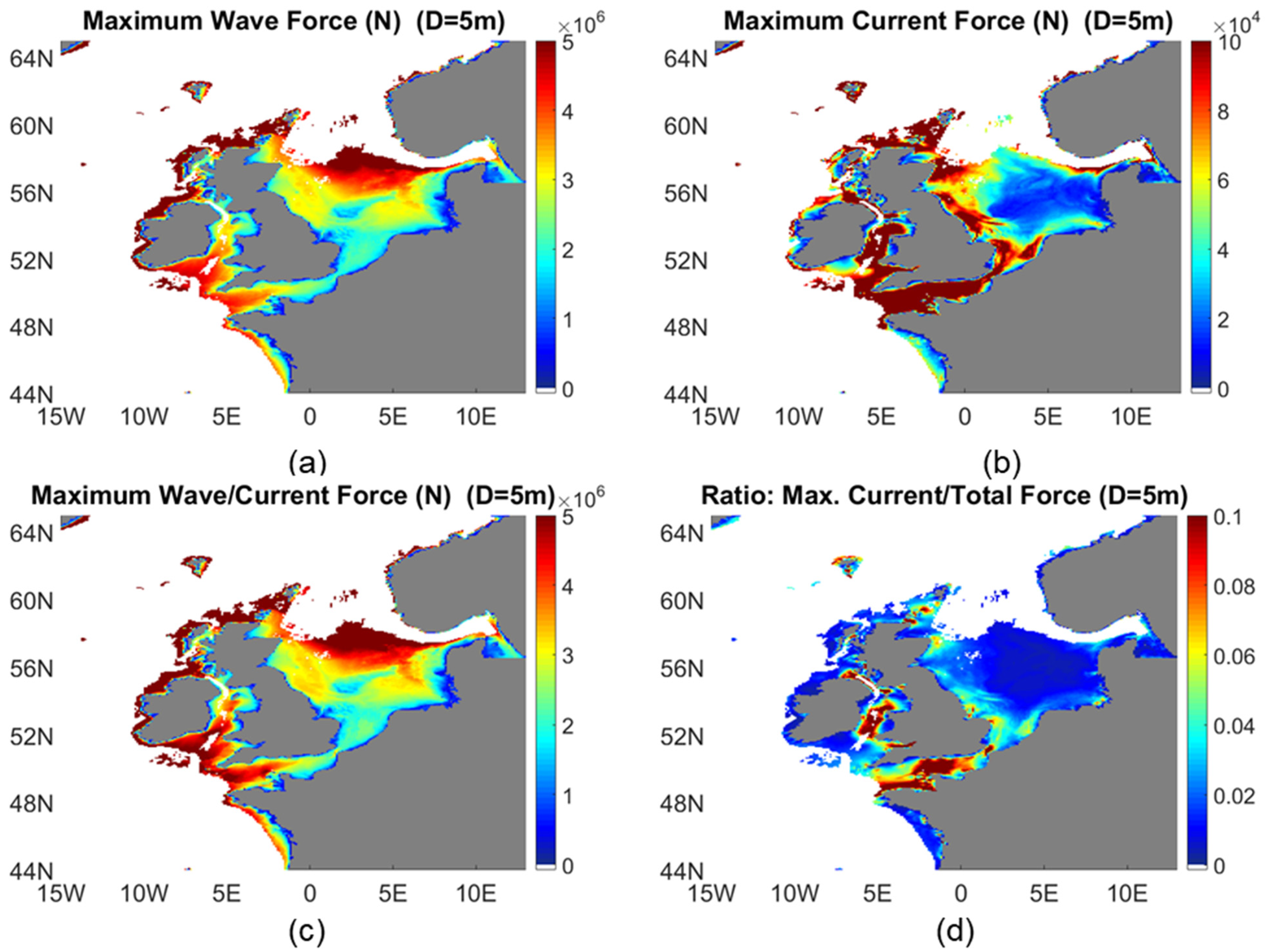
Case 2

Figure 6 shows the spatial map of maximum values of total (combined wave/current force) and the wave and current contributions to the total force on a monopile of diameter D = 5 m. This is typical of an offshore fixed wind turbine tower (submerged part). A maximum deployment depth of 100 m is considered here, although fixed wind turbine towers are typically deployed in more shallow water (<50 m depth). In general, mean and maximum force is increasing with depth as the force is integrated along the height of the monopile, which is equal to the total depth. Mean (maximum) force on the submerged monopile exceeds ~10⁶ N (5 × 10⁶ N) at the 100 m depth contour, with the western boundary showing relatively higher values as compared with the North Sea Shelf.

The wave force is at least an order of magnitude larger than the current force component largely dominating spatial variability throughout the domain. The area-averaged ratio of current to total (wave/current) force is only ~3%. Relatively large current contributions (up to 10–15%) are observed in the tidally-dominated English Channel and Irish Sea (Figure 6).

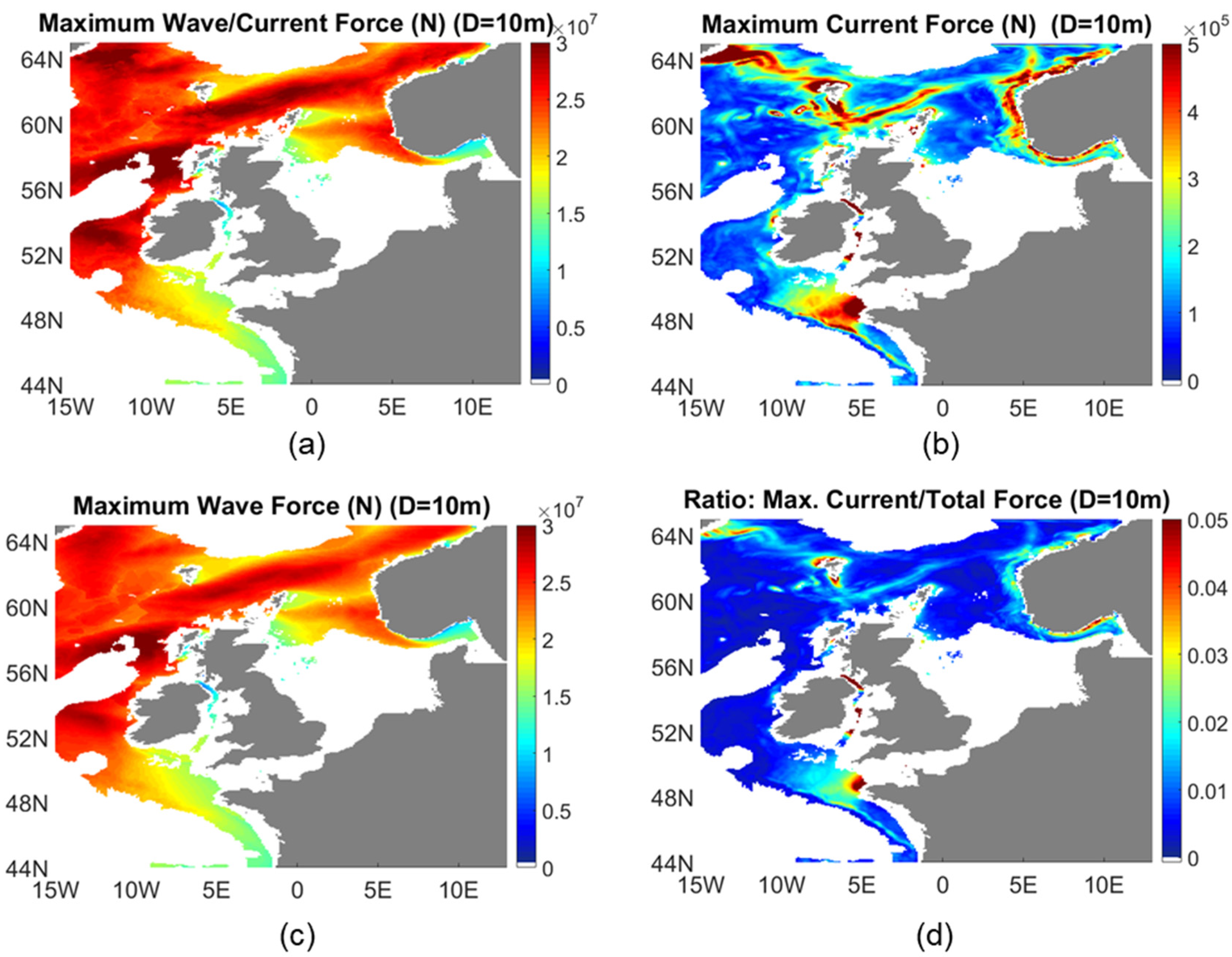
Case 3

Figure 7 shows the spatial map of maximum values of total force (combined wave/current force) and the wave and current force contributions to the total force on a floating monopile of diameter D = 10 m and of fixed height of 100 m. This is typical of an offshore floating wind turbine tower (submerged part). Therefore, the minimum deployment depth is 100 m. A maximum deployment depth of 2000 m is considered here, although floating wind turbine structures are typically deployed up to a few hundred meters depth. In contrast with fixed monopiles, the force does not depend on depth, as the height of the floating monopile is constant. Mean and maximum force on the submerged monopile exceeds ~5 × 10⁶ N and 3 × 10⁷ N, respectively obtained at the slope area around the North Sea.

The wave force is almost two orders of magnitude larger than the current force component, fully dominating spatial variability throughout the domain. The area-averaged ratio of current to total (wave/current) force is only ~1%. Larger current contributions (up to 3–5%) are observed in the entrance of the English Channel in the deep Irish Sea, and along the Norwegian Coastal Current pathway (Figure 7).

3.1.2. Temporal Variability

Time variations of hydrodynamic forces (integrated along the whole height of the pile) are assessed here in the four sub-areas (see Figure 1), representative of typical locations of offshore oil-gas and wind production support structures in the North Sea.

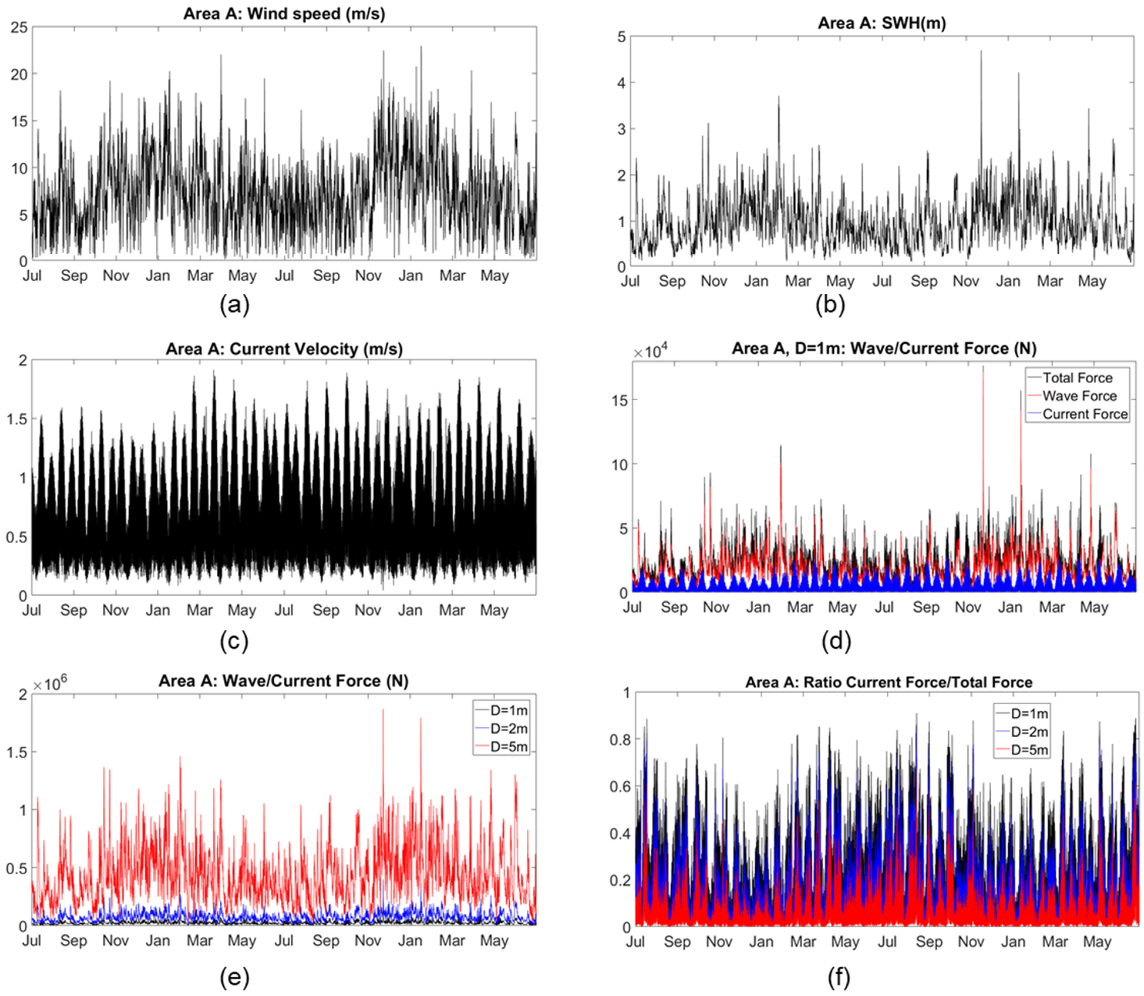
Area A (Southwestern North Sea Shelf, Average Depth = 26 m)

Figure 8 shows hourly variations of area-averaged values for area A over the period July 2014–June 2016 of the main environmental parameters (wind speed, significant wave height and current velocity) and hydrodynamic (combined wave/current, wave only, and current only) force on a cylindrical pile of 1 m diameter.

Area A is characterised by relatively low winds (mean wind speed ~7 m/s) and wave amplitudes (mean $SHW$ ~1 m). Temporal variations of these two parameters are highly correlated and show a seasonal cycle, with maximum values in winter and lower values in summer, although daily/weakly variability is very high. Storm conditions with several strong events with hourly mean wind speeds exceeding 15 m/s are obtained. However, $SHW$ peaks higher than 3 m are only observed 4 times over the 2-year period considered here. Area A is a site of strong tidal currents.

There is no visible seasonal cycle in the current velocity variations, as the tidal cycle dominates temporal variability. Mean area-averaged current velocity is ~0.7 m/s. It is interesting to note that throughout all seasons bi-monthly peaks associated with the tide exceeding 1 m/s are obtained in this area.

Mean total wave/current force over the 2-year period is ~2.3 × 10⁴ N with a few peaks exceeding 10⁵ N over strong wind events during winter. Results demonstrate that, on average, the wave contribution to the maximum load force is considerably higher than the current contribution for typical $SHW$ values, exceeding 1 m in the study area. All major total hydrodynamic force peaks, e.g., larger than 5 × 10⁴ N, are mainly attributed to the wave force. On average, the wave force contribution is ~75% of the total force in Area A. However, at low wave amplitudes ($SHW$ < 1 m), which are typical in summer, current force contribution to the total force can be higher than the wave contribution.

Mean total wave/current force over the 2-year period strongly increases with pile diameter (as both inertia and drag terms increase with $D$), from ~2.3 × 10⁴ N ($D$ = 1 m) to 7.5 × 10⁴ N for $D$ = 2 m and to 4.4 × 10⁵ N for $D$ = 5 m. It is interesting to note that the current contribution to the total force decreases as D increases, i.e., on average current contribution decreases from 25% for $D$ = 1 m to 16% for $D$ = 2 m and 8% for $D$ = 5 m.

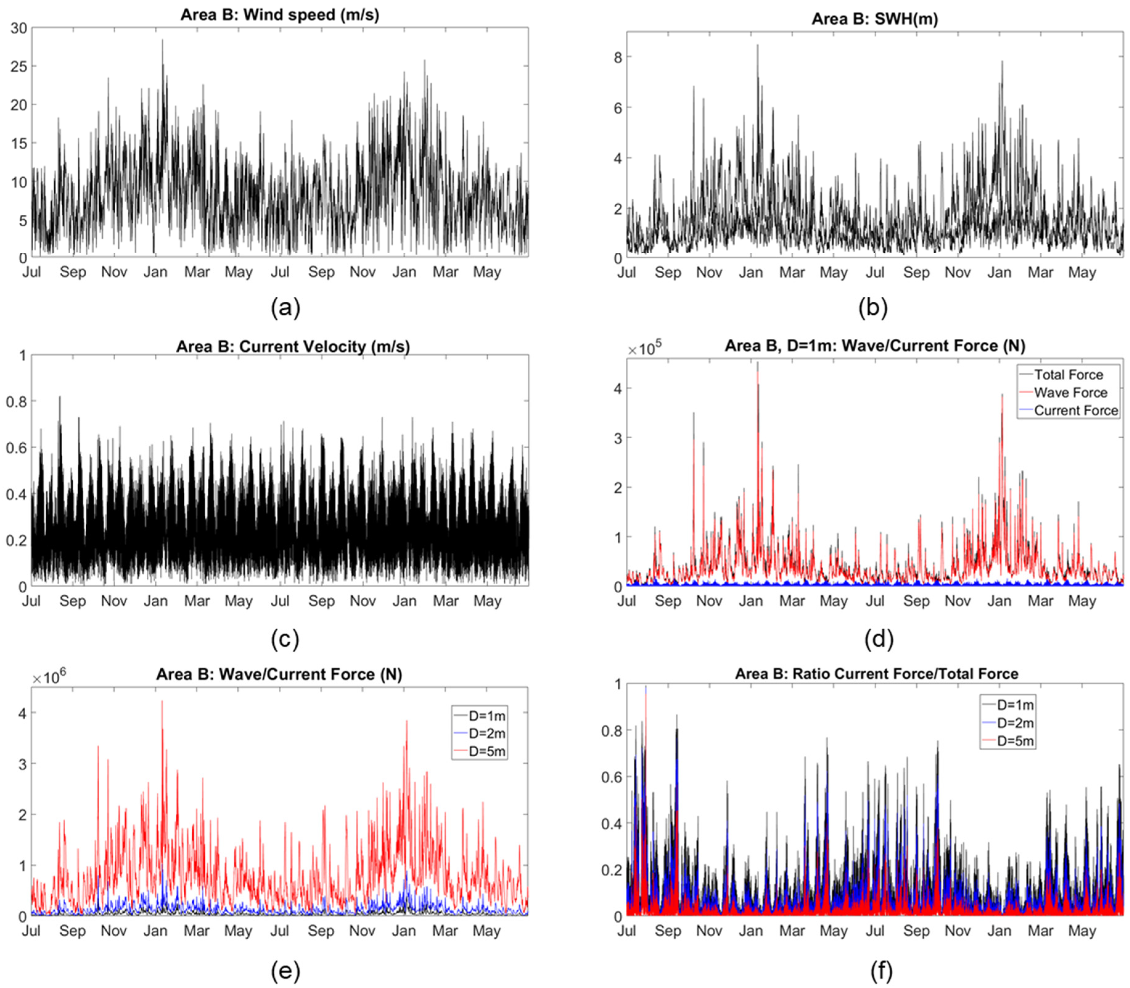
Area B (Northern North Sea Shelf, Average Depth = 92 m)

Area B is characterised by higher winds and wave amplitudes than Area A (mean wind speed ~8 m/s; mean $SHW$ ~1.9 m) (Figure 9). Wind speed and $SHW$ again show strong seasonal variations, with very high values in winter, i.e., wind speed > 20 m/s and $SHW$ > 5 m. As for area A, there is no visible seasonal cycle in the current velocity field, as the tidal cycle also dominates time variability in Area B. However, tidal impact is much lower here, with mean area-averaged current velocity of ~0.25 m/s and maximum area-averaged velocities (~0.5–0.7 m/s) being about half of those of area A. Mean total wave/current force over the 2-year period is ~4.1 × 10⁴ N. Inter-daily variability is very strong, with a few peaks exceeding 3 × 10⁵ N during strong wind events in winter.

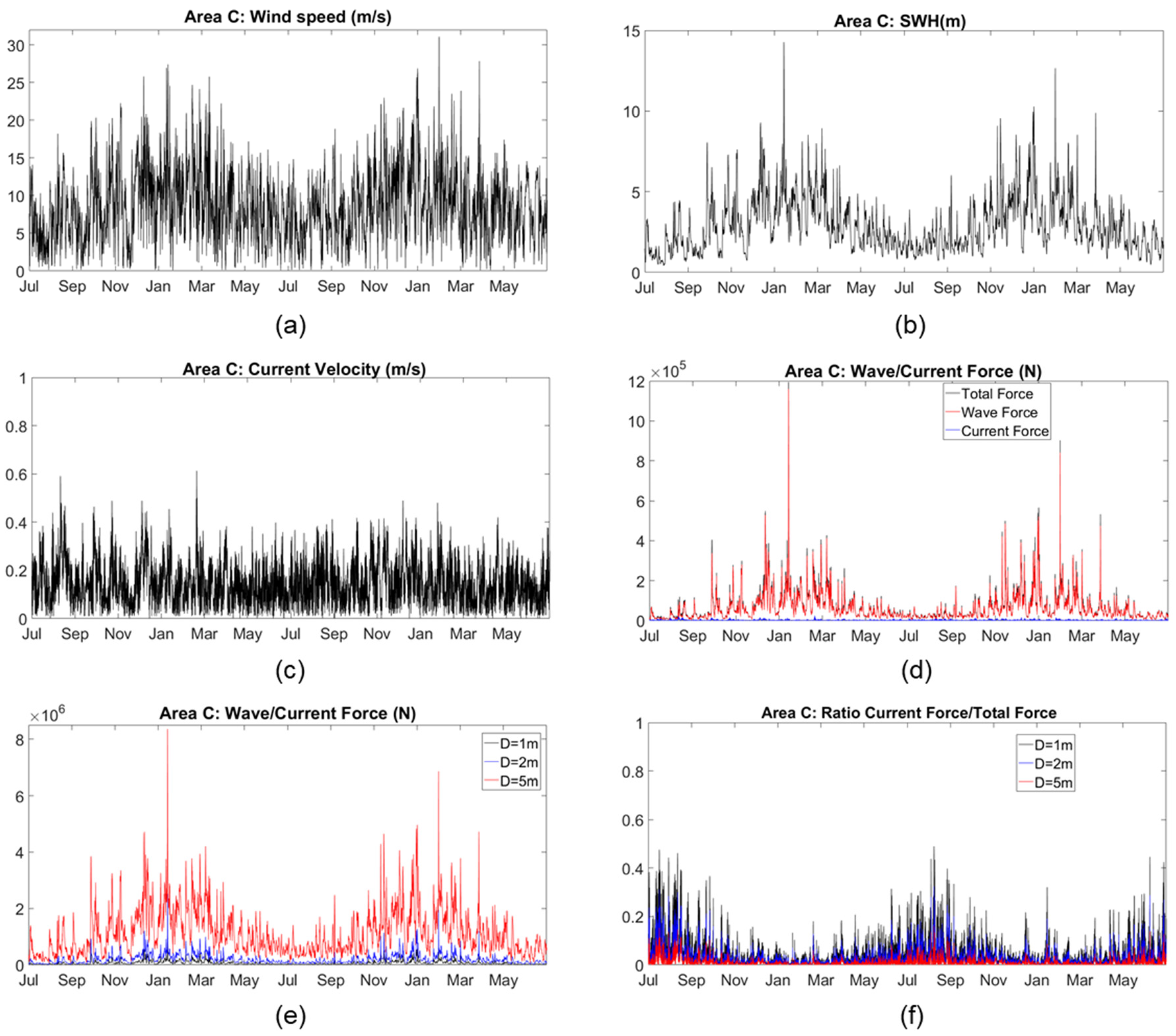
Area C (Norwegian Shelf, Average Depth = 200 m)

Area C is characterised by much higher winds and wave amplitudes than areas A and B (mean wind speed ~8.8 m/s; mean $SWH$ ~2.9 m) (Figure 10), as this is the typical entrance of storms coming from the North Atlantic into the North Sea. Wind speed and $SWH$ show very strong seasonal variations, with very high values during strong wind events in winter, i.e., wind speed > 20 m/s and $SWH$ > 7 m. Whilst current velocities can exceed 1 m/s in winter along the narrow pathway defined by the Norwegian costal current, velocities are generally low on the Norwegian Shelf, and tidal impact is very low. This results in considerably low area-averaged velocities in area C, with mean current velocity being ~0.15 m/s and maximum peaks reaching ~0.5 m/s. This is much lower as compared to tide-dominated Area A, where maximum tidal currents typically exceed 1.5 m/s.

Mean total wave/current force over the 2-year period is ~6.6 × 10⁴ N. Maximum loads during strong wind events in winter are one order of magnitude higher than the mean, exceeding 5 × 10⁵ N. Low current velocities result in very low current force, so that wave contribution is largely dominant throughout the whole time-series. On average, the wave force contribution is ~95% of the total force in Area C. Mean total wave/current force over the 2-year period strongly increases with pile diameter (Figure 10), from ~6.3 × 10⁴ N ($D$ = 1 m) to 1.9 × 10⁵ N for $D$ = 2 m and to 1.1 × 10⁶ N for $D$ = 5 m. On average, current contribution to total hydrodynamic force decreases from ~5% for a diameter of $D$ = 1 m to ~3% for $D$ = 2 m, and to only ~1% for $D$ = 5 m.

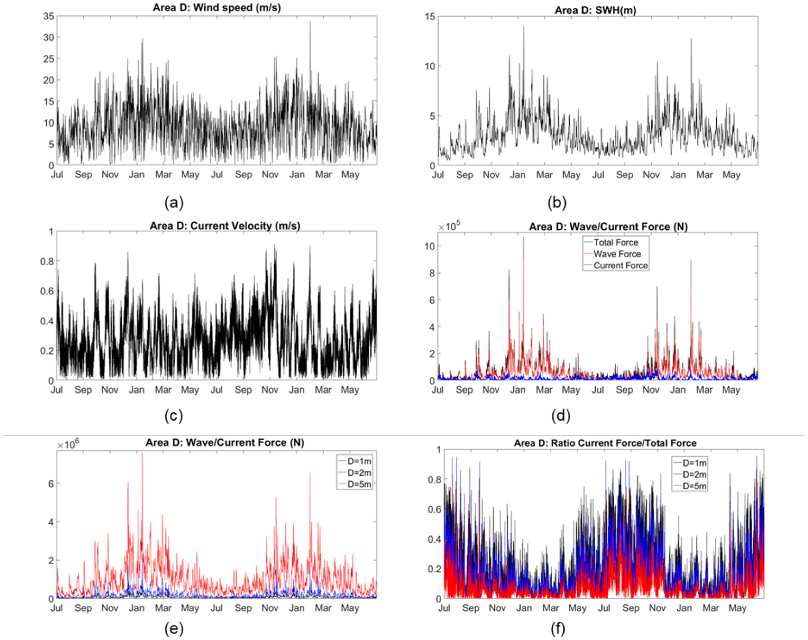
Area D (North-western North Sea Slope, Average Depth = 350 m)

Similar to Area C, Area D is also characterised by very high winds (mean wind speed ~9.3 m/s) and wave amplitudes (mean $SWH$ ~3 m) (Figure 11), as the north-western slope area of the North Sea is exposed to incoming storms from the North Atlantic. There is a very distinct seasonal cycle, with strong wind events in winter, when wind speed > 20 m/s and $SWH$ > 7 m. Although tidal impact is very small, current velocities are strong in the slope area and highly correlated to the wind speed. Mean area-averaged current velocity is ~0.2 m/s, with maximum values exceeding 0.7 m/s during strong wind events. Mean total wave/current force over the 2-year period is ~6.6 × 10⁴ N. Maximum loads during strong wind events in winter are one order of magnitude higher than the mean, exceeding 5 × 10⁵ N. Although currents considerably contribute to the total hydrodynamic force, wave contribution is still dominant in this area, at about 78% on average.

Mean total wave/current force over the 2-year period strongly increases with pile diameter (Figure 11), from ~6.6 × 10⁴ N ($D$ = 1 m) to 1.9 × 10⁵ N for $D$ = 2 m and to 1 × 10⁶ N for $D$ = 5 m. On average, current contribution to total hydrodynamic force decreases from 22% for a diameter of $D$ = 1 m to 14% for $D$ = 2 m, and to 7% for $D$ = 5 m.

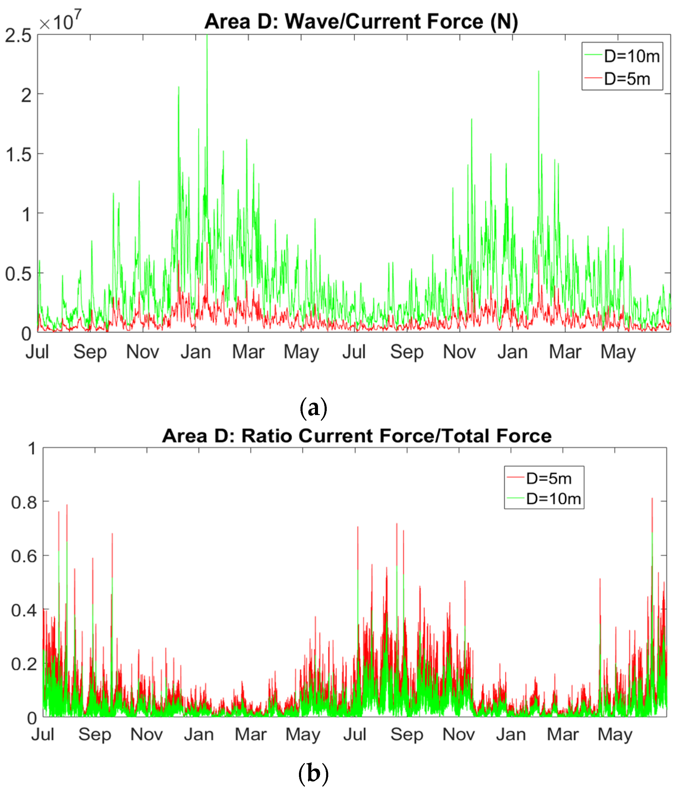
For the case of floating structures with a typical diameter of the submerged pile of 10 m, the hydrodynamic force mean value is 3 × 10⁶ N, whilst total hydrodynamic force can reach extreme values of 2–2.5 × 10⁷ N during severe storms (Figure 12). Maximum hydrodynamic force is about five times larger, as compared with a floating pile of a diameter of 5 m. On average, current contribution to total hydrodynamic force is much lower, i.e., ~3% as compared to a pile of 5 m diameter (~7%).

3.2. Wind Drag Force

We now address the wind drag force on the exposed part of a structure, assessed both spatially and temporally, with a focus on demonstration case 2.

3.2.1. Spatial Variability

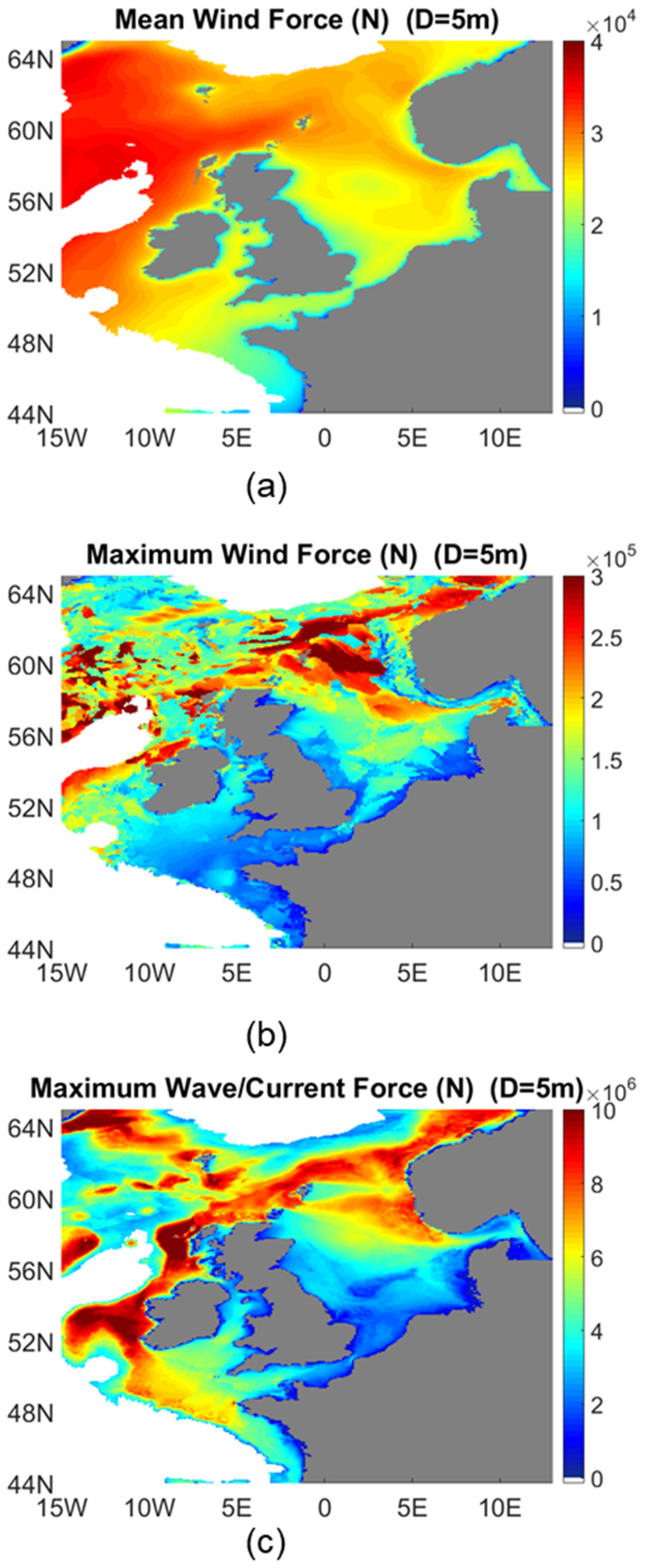
Spatial variability of wind drag force is presented here by spatial maps (NW European Shelf area) of temporal mean and maximum values (in Newtons) over a 2–year period (July 2014–June 2016). The wind drag force is integrated along the whole height of a wind turbine tower, here defined as a cylindrical pile of constant diameter of 5 m and above sea level height of 100 m that is constant throughout the whole domain covering 0–2000 m depth. Wind drag mean/maximum force distribution is fully explained by mean/maximum wind speed distribution (see Figure 2). Mean wind drag force (Figure 13) increases from the southern part of North Sea Shelf (~2 × 10⁴ N) to the slope (~3 × 10⁴ N) and then the deep ocean (~4 × 10⁴ N) following a north-westward gradient. Maximum wind force over the considered period is obtained along the slope area following the north-eastward pathway of storms in the North Atlantic. Within the North Sea, there is a strong north-eastward gradient of increasing force from the UK east coast (~5 × 10⁴ N) to the northeast part of the slope area (~3 × 10⁵ N). Note that for the same pile diameter (D = 5 m), the hydrodynamic maximum force is spatially correlated with the maximum wind drag force, but the latter is at least one order of magnitude lower throughout most of the area (Figure 13c). In the case of floating (spar type) wind towers (Case 3) where the diameter of the submerged part of the pile is 10 m, the total hydrodynamic force is approximately two orders of magnitude larger than the wind drag force on the above-sea level tower of 100 m height.

3.2.2. Temporal Variability

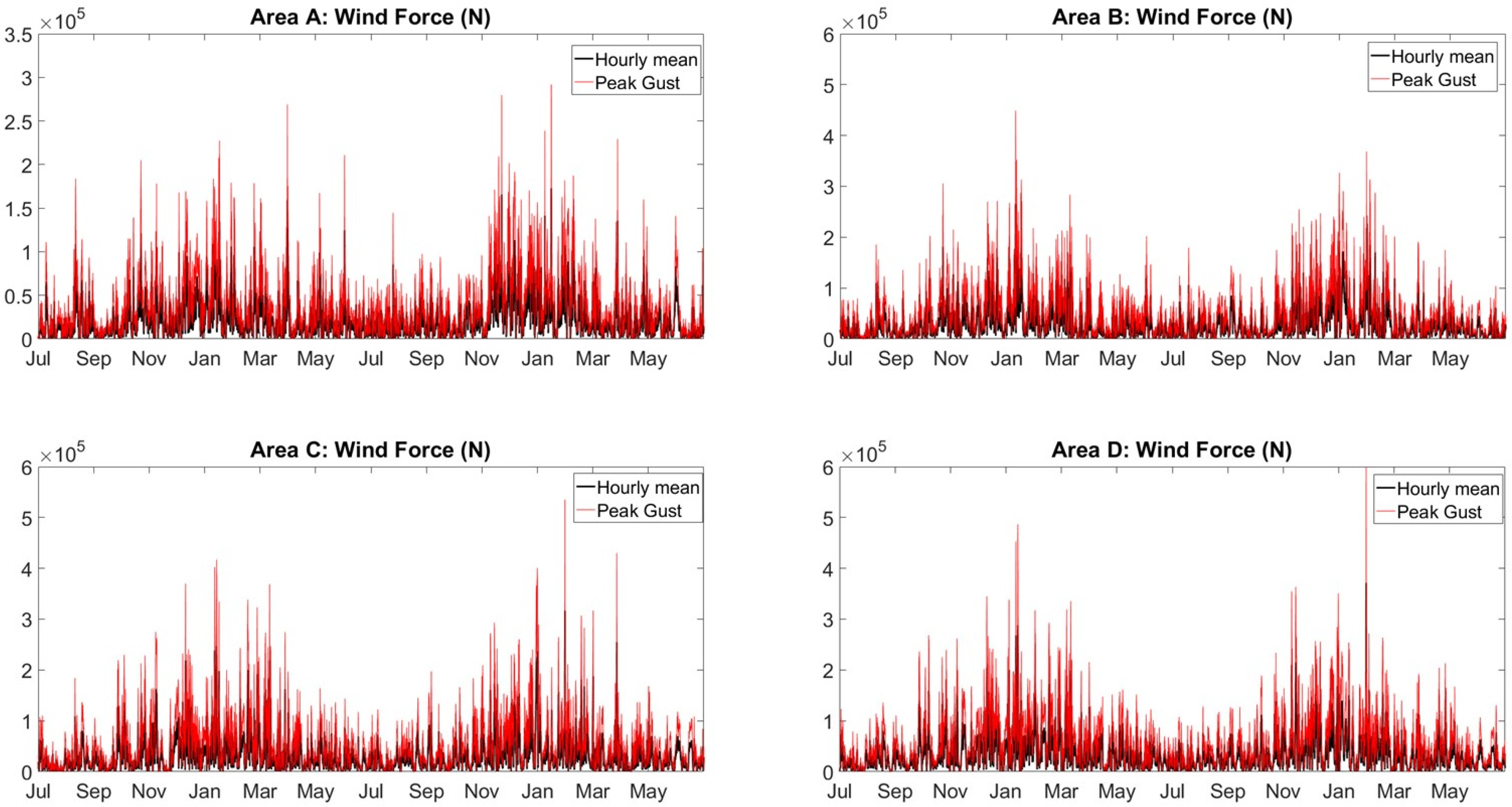
Similar to hydrodynamic forces, time variations of the wind drag force (integrated along the whole height of the above sea level pile) is assessed here in the four sub-areas (see Figure 1). Figure 14 shows hourly variations of area-averaged hourly mean and peak gust (i.e., maximum over 3 s) values of the wind drag force on a cylindrical pile of 5 m diameter for the four sub-areas over the period July 2014–June 2016. As expected, variations of the area-averaged wind drag force closely follow wind speed variations. There is a very distinct seasonal cycle in all sub-areas with larger mean hourly force and more intense extremes during strong wind events in winter where wind speed exceeds 15 m/s. Mean hourly wind drag force is significantly lower in Area A within the southern North Sea shelf where winds are low (~2.2 × 10⁴ N), with respect to the three other sub-areas, i.e., area B within the northern North Sea shelf (~3.0 × 10⁴ N), area C in the Norwegian Shelf (~3.2 × 10⁴ N) and area D along the slope (~3.4 × 10⁴ N) associated with much higher wind speeds. There is strong inter-daily variability with the hourly wind drag force exceeding 10⁵ N during strong wind events in all sub-areas. Peak gust force is approximately 70% higher than hourly mean wind force. Maximum hourly wind and peak gust drag force over the whole period of ~ 3.6 × 10⁵ N and 6 × 10⁵ N, respectively, is obtained in Area D in January 2016.

3.3. Impact of Model Spatial Resolution on Wave and Current Loads

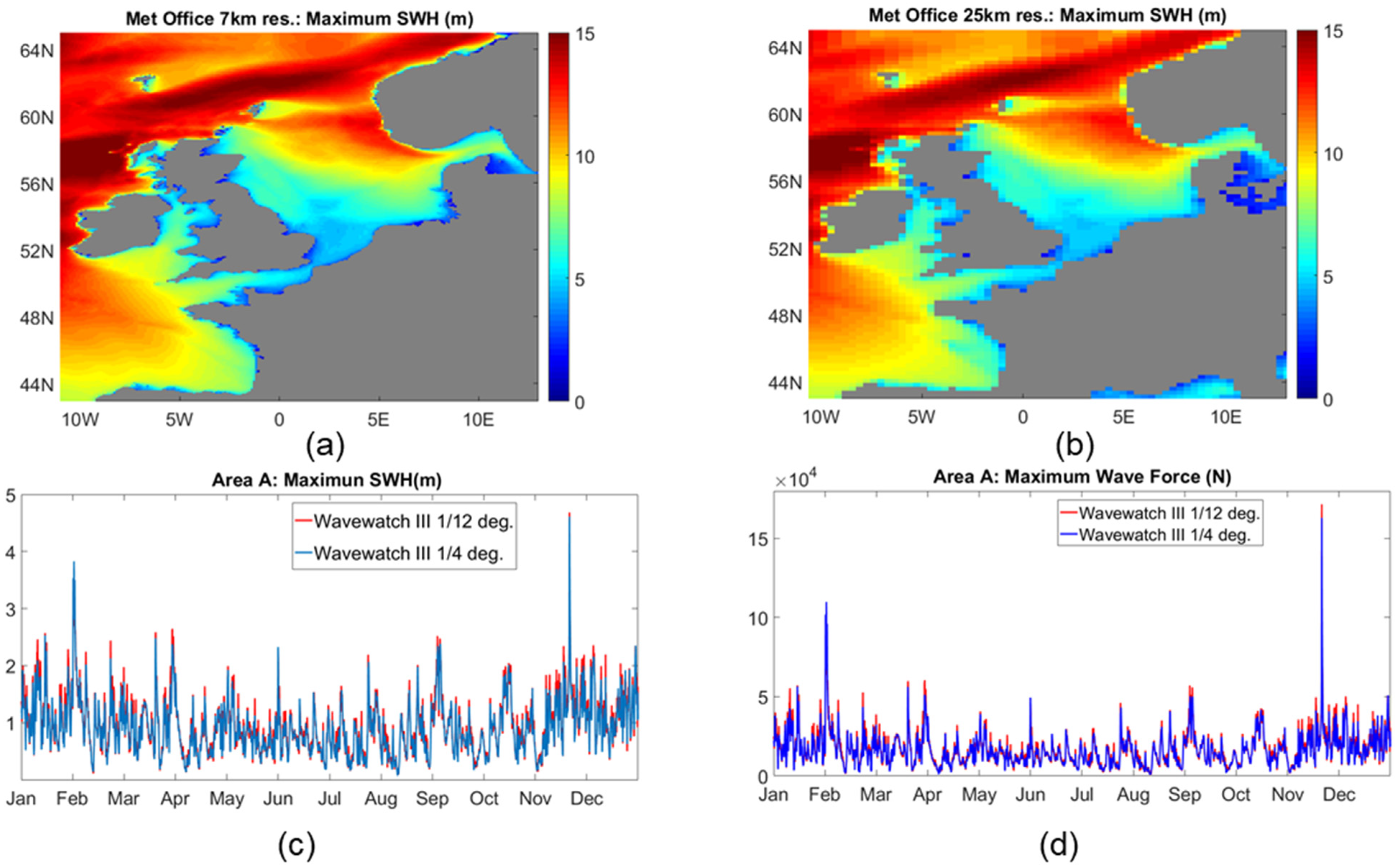
Results show that spatial resolution of the wave model (WaveWatch III) has a small impact on the estimated wave loads on offshore structures. Figure 15 shows NW European shelf area maps of annual maximum significant wave height for the two Met Office wave products used here, i.e., the ~7 km and ~25 km spatial resolution products, respectively. Maximum significant wave height distribution is very similar at the two resolutions, with higher resolution wave model producing slightly higher values locally as spatial extremes are smoothed out in the low-resolution model.

Mean and maximum wave force time variations are almost perfectly correlated between high- and low-resolution products. The resulting maximum wave force integrated along a cylindrical pile of 1 m diameter is, on average, only ~10% larger in the high-resolution model as compared to the low-resolution model (Figure 16).

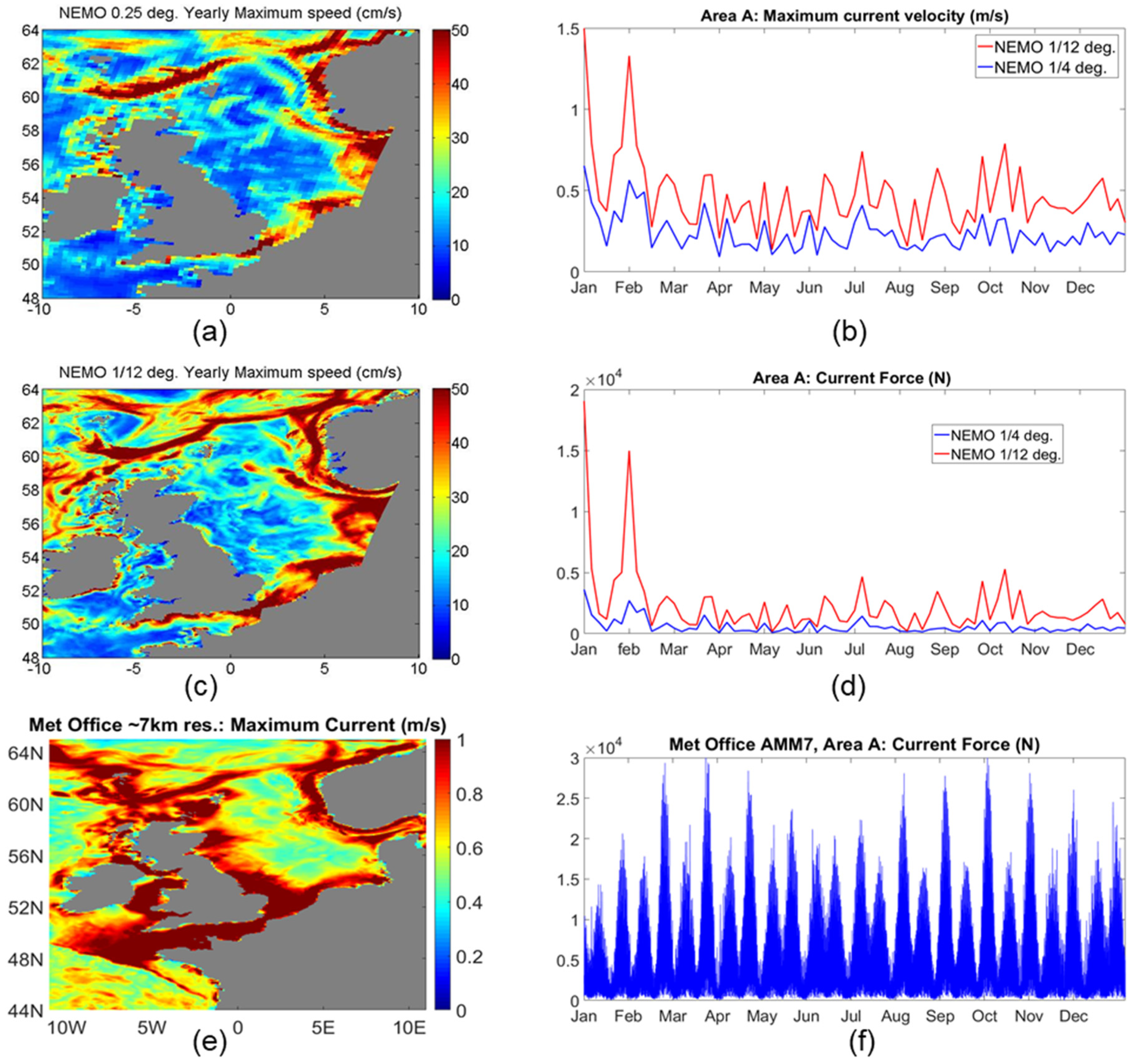
The impact of ocean circulation model spatial resolution cannot be fully assessed here as we only use the high-resolution version of the Met Office ocean operational model (~7 km). However, results based on the NOC NEMO ocean model hindcast with ORCA12 (1/12° resolution, ~7 km) and ORCA025 (1/4° resolution, ~25 km) horizontal mesh versions demonstrate that ocean circulation model spatial resolution has a strong impact on the estimated current loads on offshore structures (Figure 16). Compared with ORCA12, currents in ORCA025 are broader and weaker. Overall, ORCA12 is more realistic. There is generally more variability and higher maximum current intensity in ORCA12. The maximum current speed is, on average, about 60% higher in the ORCA12 hindcast as compared to ORCA025 hindcast. However, in wintertime, when ocean circulation is more intense, maximum current speeds can be up to twice as high in ORCA12 as compared to ORCA025. As a result, on an annual basis, the maximum current force in the North Sea is, on average, more than twice as high when using ORCA12 as compared to ORCA025. The obtained force can be up to five times higher in ORCA12 when maximum current velocities exceed 1 m/s.

Although the ocean hindcast (NOC) and Met Office FOAM AMM7 ocean model systems are based on the same ocean model (NEMO), there are significant differences in their settings. In the Met Office NEMO Operational nowcast/forecast system, various observational ocean data are assimilated to provide more realistic initial conditions, whereas the atmospheric forcing is taken from a high-resolution weather prediction model providing high-frequency boundary conditions, and, importantly, high-frequency tidal motion is simulated. In the NEMO hindcast model, the ocean is forced by an atmospheric re-analysis, which assimilates ocean surface observations, but at low resolution in both space and time, whereas tidal currents are not simulated. An advantage is that there is the availability of a long-term hindcast spanning several decades (from 1978 until present), while there are no problematic or ill-conditioned boundary conditions imposed by a nesting procedure, as the model is global at the maximum (1/12°) resolution.

In general, there is more temporal variability and maximum currents are much stronger in FOAM, compared to the hindcast (see Figure 16). This suggests that assimilating daily observations in FOAM, and especially the inclusion of tidal currents, strongly enhances temporal variability of currents realistically representing maximum currents. At the same spatial resolution (1/12°), the operational FOAM model produces significantly higher maximum current force as compared to ocean hindcast throughout the NW European shelf seas (on average two times higher), whereas maximum force is several times higher in the Irish Sea and Southern North Sea, where maximum tidal current velocities typically exceed 1.5 m/s.

4. Conclusions

This study refines and extends the use of the Morison equation to assess the combined wave/current/wind loading imposed on fixed and floating cylindrical/tubular structures typically employed in the North Sea, based on high-resolution Met Office operational forecast data. Results indicate that waves dominate extreme hydrodynamic forces on the shallow shelf, whereas the current contribution is important at the shelf break and in the English Channel, characterized by strong slope and tidal currents, respectively. Our analysis for the fixed 100 m tall monopiles with diameters 5–10 m in the North Sea demonstrated that the wave force is, on average, at least an order of magnitude larger (~50 MN for 10-m diameter structure) than the current force, especially over the shallow continental shelf, where the wave force largely dominates the total hydrodynamic load on all types of offshore structures. A relatively larger current contribution is obtained in the tidally dominated areas, such as the English Channel (~1 MN for 10 m diameter structures), or in deeper regions, and over the continental slope, where currents typically exceed 1 m/s.

Hydrodynamic force temporal variations indicate a clear seasonal cycle with the hydrodynamic force acting on all offshore structures showing minimal values in summer and maximum values in winter, closely following wave amplitude seasonal variations, with much larger waves obtained during winter. However, timeseries also reveal much stronger higher frequency variability. Over the 2-year period considered here, extreme total (wave/current) hydrodynamic force can exceed, by an order of magnitude, the climatological mean force for both fixed and floating structures.

Results show that wind turbines on the slope area can benefit by much higher mean wind speeds i.e., up to two times higher mean wind speeds compared to coastal shelf regions of the North Sea, which may result in considerably larger wind power generation. However, the north-western slope area of the North Sea is also exposed to incoming storms from the North Atlantic and to permanent strong slope currents. Extreme hydrodynamic loads on the monopile support (spar type) structure of wind turbines considerably increase in deeper areas, and they can be an order of magnitude higher in and around the shelf break compared to coastal/shelf regions. The wind drag force is spatially correlated with, but much lower than, the hydrodynamic force, in the slope and in deeper areas in particular, where the latter is ~2 orders of magnitude stronger.

Spatial resolution of the wave model has a very small impact in the calculation of wave loads. We surmise that this is due to the wind forcing being the key factor controlling wave spatiotemporal variability in the present model and it does not change between the resolutions. In contrast, the ocean model resolution is of crucial importance for ocean circulation models to properly represent current loads on offshore structures. Maximum current speeds can be up to twice as high in the NEMO hindcast, and the associated maximum current load can be up to five times higher when model horizontal resolution increases from a 1/4 to 1/12 of a degree. The ocean model resolution effects are due to the higher resolution model configuration being able to resolve mesoscale eddy dynamics and associated with eddies higher peak velocities.

The study also underlines the advantages of using operational forecasts compared to ocean hindcast simulations to properly assess the hydrodynamic loads on offshore structures. Operational forecast systems which assimilate high-frequency observations and especially include tidal forcing can represent, more realistically, the temporal variability of ocean circulation and especially extreme currents. At the same spatial resolution, and based on the same ocean model, the Met Office operational forecasting system used here produces significantly higher maximum current loads compared to ocean hindcasts throughout the NW European shelf seas and can be several times higher in tidally dominated areas, such as the Irish Sea, the English Channel and Southern North Sea.

We need to stress the limitations of the ME method applied here to calculate hydrodynamic loads, using simplified geometrical parameters of structures and the representation of wave dynamics. In particular, wave diffraction is neglected, and this process may be important in larger diameter monopiles typically used to support offshore wind turbines [3]. In particular, the case of 10 m diameter for a floating monopile used here is at the limit of the ME method applicability. Moreover, relative structure displacement is neglected here, and this process can be especially important for floating (spar type) structures.

Another caveat concerns the spatial resolution of ocean models producing the current field to calculate the current load on the offshore structure. In particular, inertial currents associated with passing storms that drive near-surface currents of typically 0.5–1 m/s are not resolved in the model products used here. The spatial resolution of the most advanced ocean hindcast or operational forecast systems at regional scale is of an order of a few kilometres, such that the simulated current regime is still probably not fully representative of the current regime around an offshore structure, with a typical length scale of the order ~10–100 m. A model downscaling/nesting technique providing a much higher resolution around the structure is therefore required to be able to solve small-scale processes and their impact on hydrodynamic loads. Moreover, a high-turbulent wind pattern can have a large impact on wind turbine support structures, and the relatively simple empirical formulas used here to extrapolate the wind profile and estimate the wind gust based on hourly mean wind data are probably not sufficient to capture the complexity of the wind field. Therefore, higher frequency wind data and advanced turbulent models are needed to better assess extreme wind drag loads on these structures.

Furthermore, other processes which are not investigated here and need to be assessed in the future, including heave excitation and buoyancy forces [32], and vortex-induced vibrations on floating structures are part of the design process and can have strong impacts on structural integrity. In general, the fully coupled integrated structural response of fixed and floating offshore structures to extreme environmental conditions needs to be assessed [5,33].

In this demonstration case study, we calculate mean and maximum environmental loads on the offshore structures of different types, using only 2 years of wave/current/wind data provided by the Met Office forecasting system. Although this period provides the basic seasonal statistics of environmental loads and highlights intra-annual frequency of extreme events, it is too short to be able to produce a meaningful statistical analysis of the extremes characterised by much longer return periods. Nevertheless, this study demonstrates the importance of synthesizing high-quality environmental data, to improve our knowledge of the statistics of extreme environmental forces acting on offshore structures. In particular, Met-Ocean data of high spatial resolution and frequency output used here allow one to establish the spatial variability and the seasonal cycle of environmental forces on various types of structures, and therefore can give valuable information about the expected place and time occurrence of extreme loads in the North Sea. Moreover, the present methodology based on ocean re-analysis data could be used in the future to construct longer timeseries of environmental loads suitable for a valid statistical analysis of the extremes. Current ocean re-analysis models running in hindcast mode can cover periods of ~40–50 years, typically from the late 1970s with the start of the satellite ocean observation era. However, to capture longer return periods, this approach needs to be complemented with an analysis of available in situ data long-term timeseries.

Our results demonstrate that a state-of-the-art system based on a wide range of research and operational expertise is required to inform the safety and risks of the employment of offshore structures concerning structure integrity design criteria and operational activities around the global ocean. In particular, we need to integrate the high-quality hindcasts and forecasts of ocean currents, tides and waves, in a variety of environments, including the effects of sea ice in high latitudes, where the emerging changes in the sea ice and oceanic environment pose new risks for offshore operations and challenges for forecasting [34,35]. In this way, we can provide the best possible advice on forces and environmental conditions experienced by offshore structures at regional and global scales of considerable importance to the economy of many countries around the world. In a multidisciplinary context, our environmental load analysis should be combined with the analysis of other indices, such as seabed conditions, visibility, and maritime transport traffic, to better inform the evaluation of offshore structure deployment sites.

In developing the throughput and use of ocean state and wave forecasting data, these assessments may also be of use in real-time offshore operations. The real-time calculation of the forces acting on specific structures at high spatial resolution and frequency, based on high-resolution operational wind, ocean, and wave forecasts, holds promise for operational use by classification societies and offshore operators. The indirect cost benefits may be considerable through reductions in marine losses and damages. Moreover, these assessments may also help to raise safety standards around the offshore industry.