Dynamics of the Land–Sea Breeze System and the Surface Current Response in South-West Australia


Abstract
:1. Introduction
Study Region
2. Materials and Methods
2.1. Field Measurements
2.2. Numerical Models
2.3. Analysis Techniques
3. Results
3.1. Measurements: Rottnest Island Meteorological Station
3.2. WRF Model Output
3.3. Surface Currents from HF Radar
3.4. ROMS Model Output 4
3.5. Diurnal Ellipse Characteristics from WRF and ROMS Models
4. Discussion
5. Conclusions
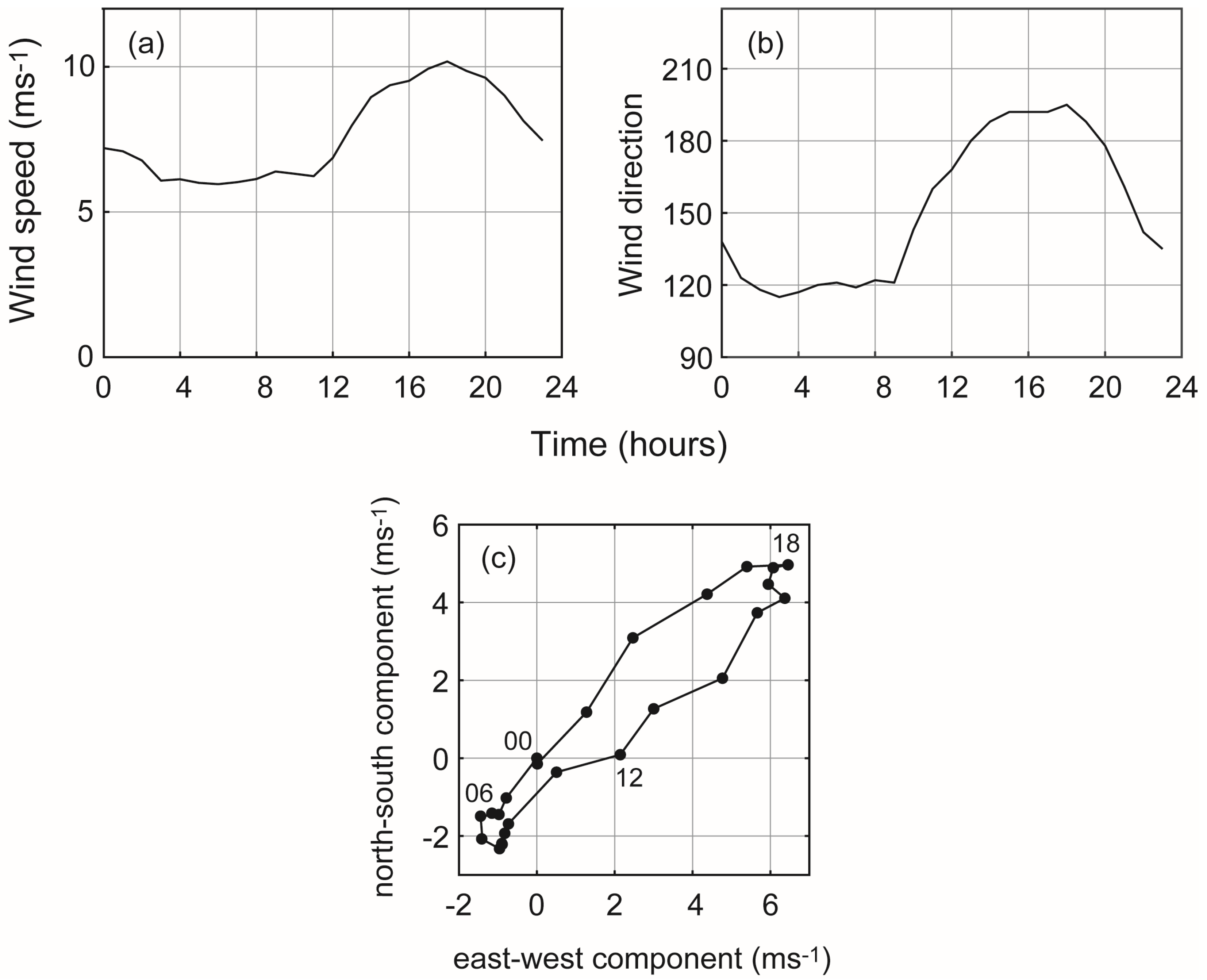
- (a)
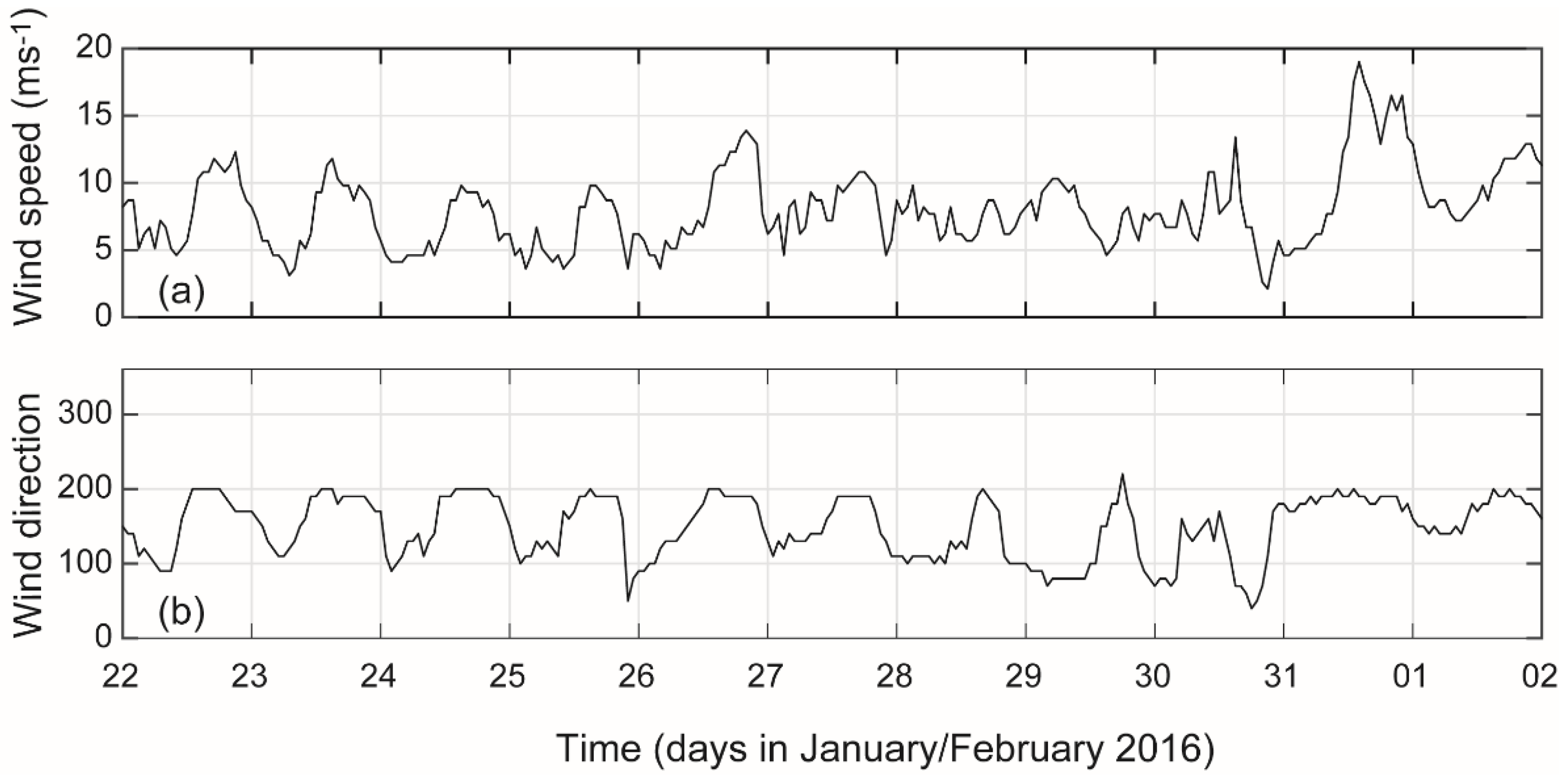
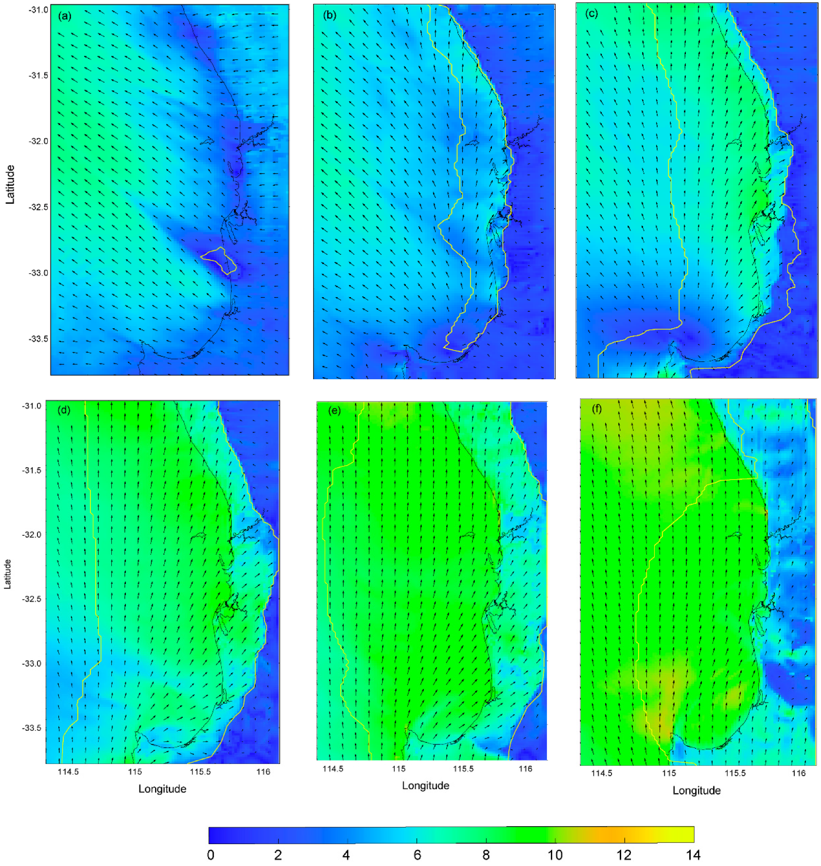
- The LSB cycle was such that wind speeds decreased between midnight and 0400 and increased rapidly after 1100, reaching maxima >10 ms−1 around 1800, decreasing to midnight. Wind directions were such that there were southeasterly winds (120°) in the morning and changing to southerly (~200°) in the afternoon. Although the sea breeze winds (diurnal) were oriented south-west to north-east in combination with the south-easterly gradient winds resulted in the southerly direction.
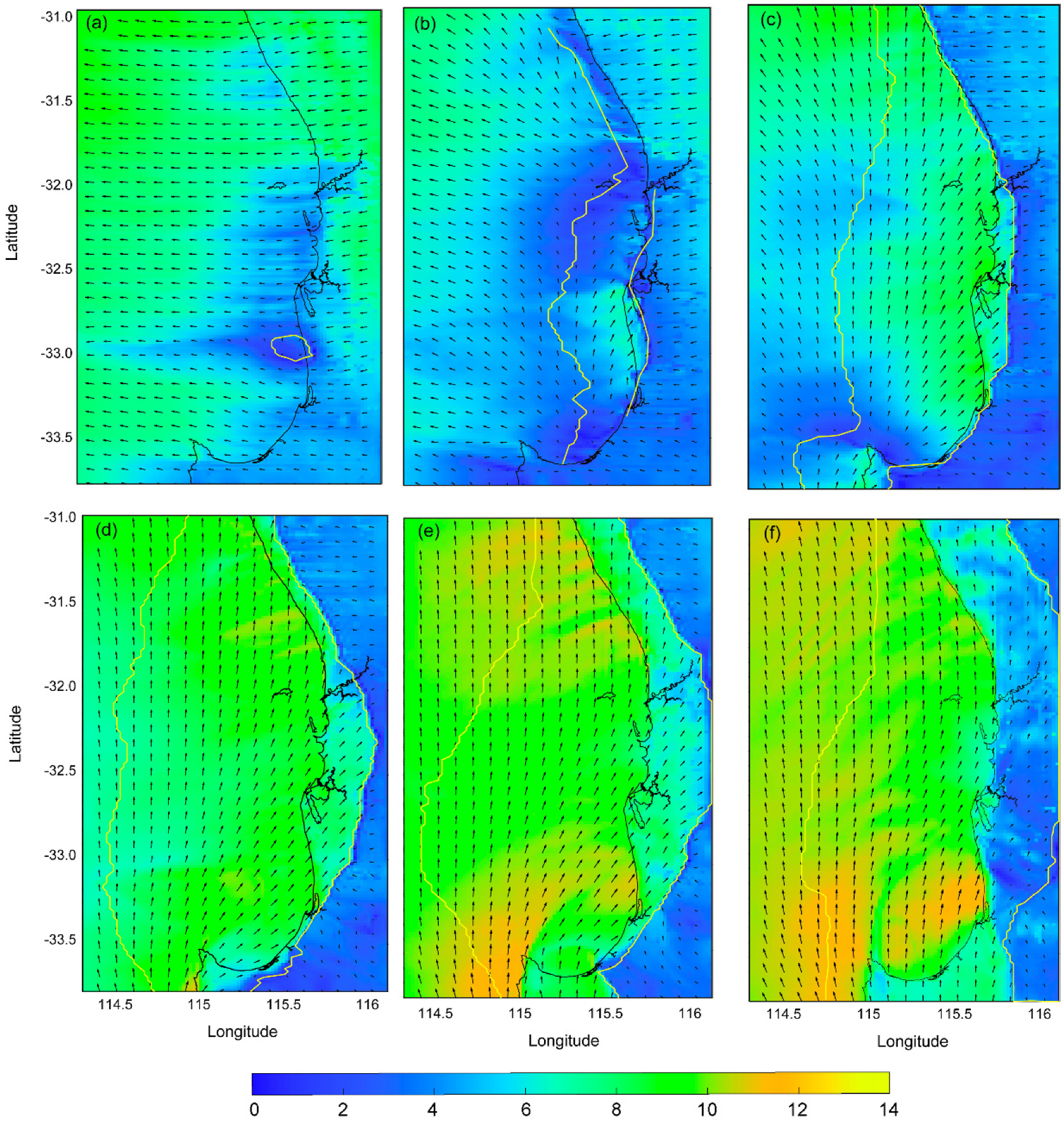
- (b)
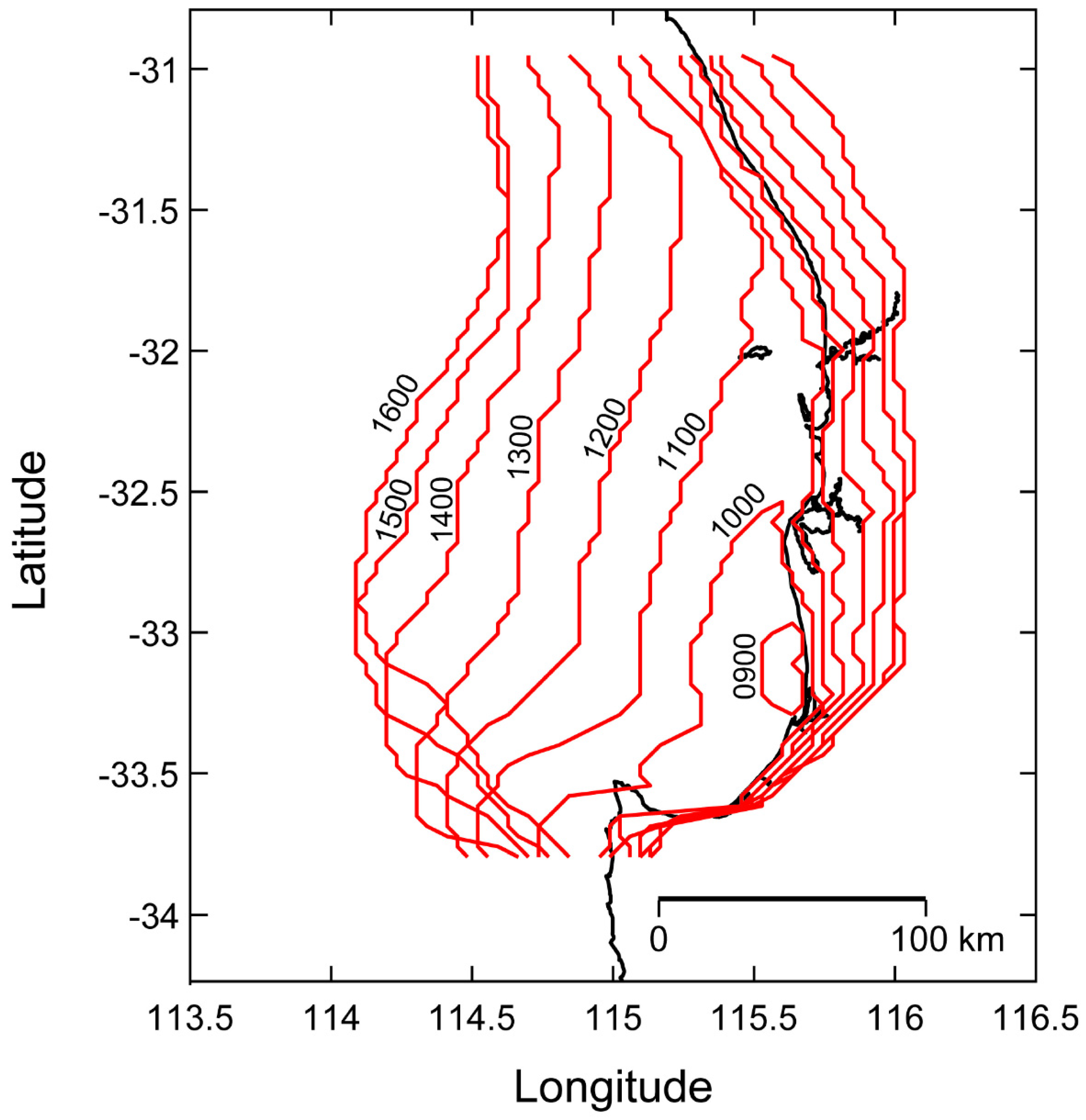
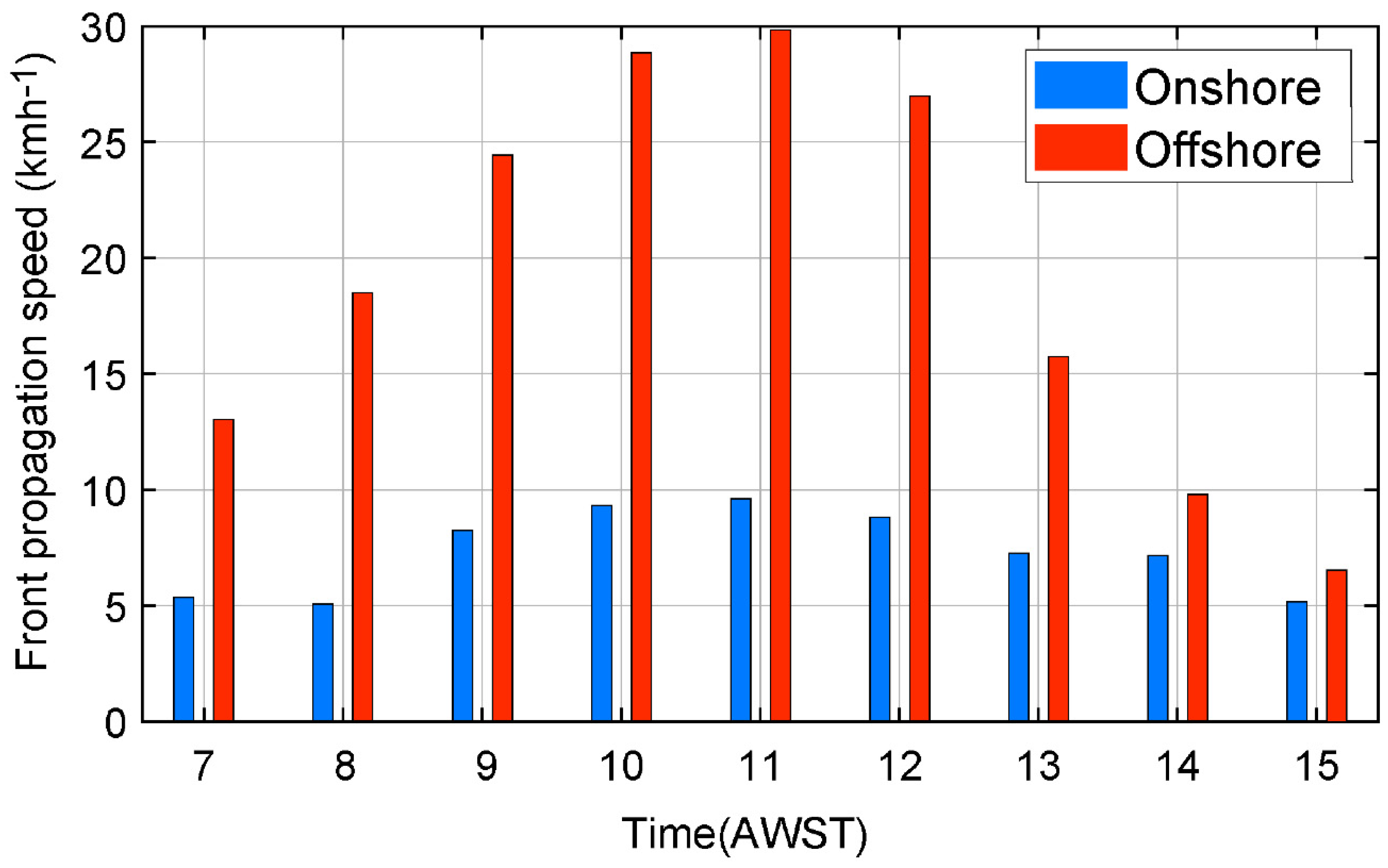
- The sea breeze cell was initiated within a small area near 115.5° E; 33° S in the morning around 0800 and expanded asymmetrically offshore with maximum speed of 30 kmh−1 reaching 120 km offshore. In contrast, the onshore propagation was limited to 30 km at a maximum speed of 10 kmh−1.
- (c)
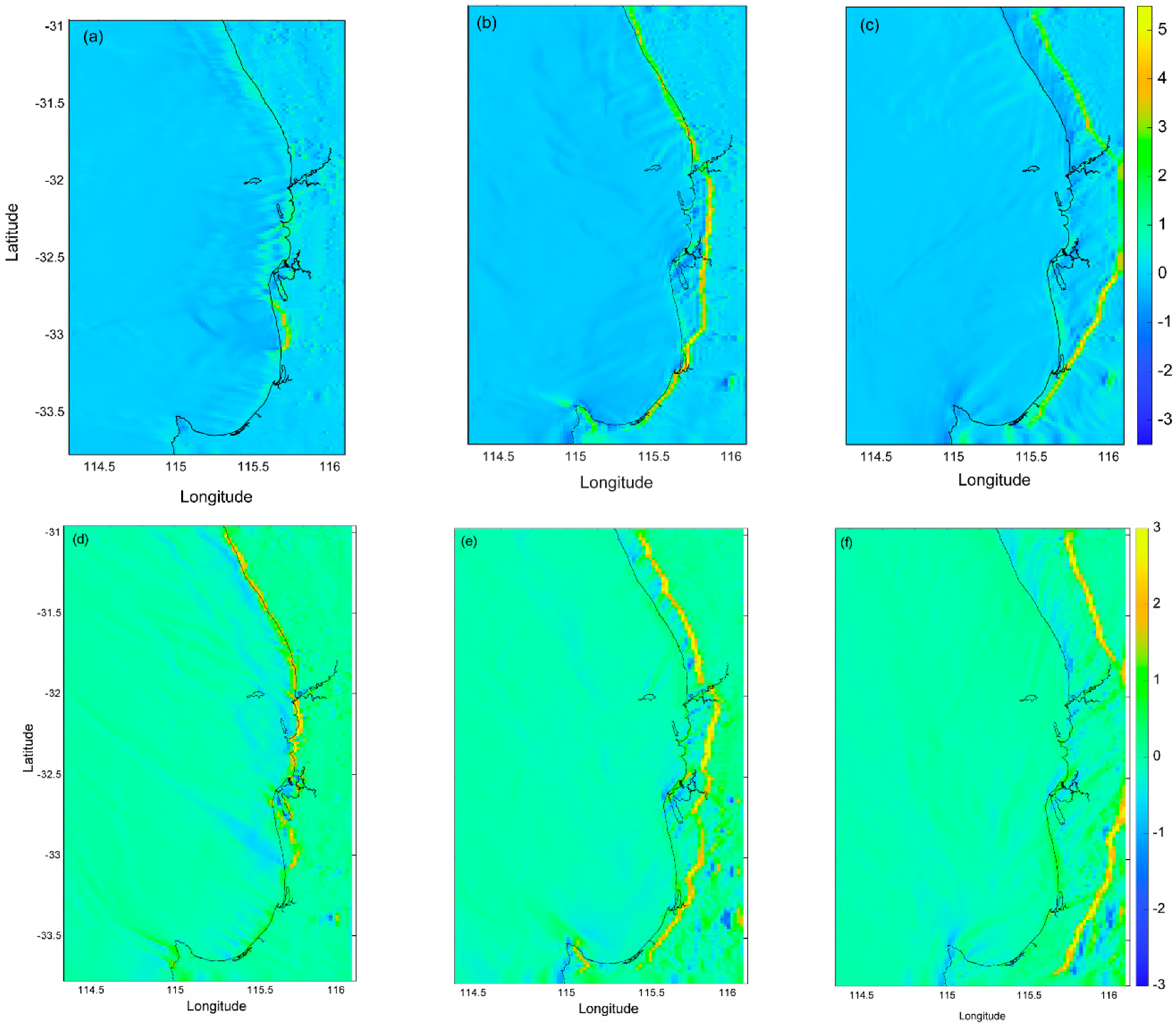
- The wind and surface currents rotated anticlockwise with the surface currents responding almost instantaneously to changes in wind forcing but were modified by topography.
Author Contributions
Funding
Conflicts of Interest
References
- Sonu, C.J.; Murray, S.P.; Hsu, S.A.; Suhayda, J.N.; Waddell, E. Sea breeze and coastal processes. Eos Trans. Am. Geophys. Union 1973, 54, 820. [Google Scholar] [CrossRef]
- Neumann, J. The Coriolis Force in Relation to the Sea and Land Breezes—A Historical Note. Bull. Am. Meteorol. Soc. 1984, 65, 24–26. [Google Scholar] [CrossRef] [Green Version]
- Simpson, J.E. Diurnal Changes in Sea-Breeze Direction. J. Appl. Meteorol. 1996, 35, 1166–1169. [Google Scholar] [CrossRef]
- Davis, W.M.; Schultz, L.C.; Ward, R. An investigation of the sea breeze. Harv. Univ. Ann. Astron. Obs. 1890, 21, 214–264. [Google Scholar]
- Simpson, J.E. Sea Breeze and Local Winds; Cambridge University Press: Cambridge, UK, 1994; 234p. [Google Scholar]
- Miller, S.T.K.; Keim, B.D.; Talbot, R.W.; Mao, H. Sea breeze: Structure, forecasting, and impacts. Rev. Geophys. 2003, 41. [Google Scholar] [CrossRef] [Green Version]
- Masselink, G.; Pattiaratchi, C.B. Characteristics of the sea breeze system in Perth, Western Australia, and its effect on the nearshore wave climate. J. Coast. Res. 2001, 17, 173–187. [Google Scholar]
- Dampier, W. Voyages and Descriptions, Vol. II: Capt. Dampier’s Discourse of the Trade Winds, Breezes, Storms, Seasons of the Year, Tides and Currents of the Torrid Zone Throughout the World; Printed for James Knapton: London, UK, 1705; p. 112. [Google Scholar]
- Abbs, D.J.; Physick, W.L. Sea breeze observations and modelling: A review. Aust. Meterological Mag. 1992, 41, 7–19. [Google Scholar]
- Pattiaratchi, C.B.; Hegge, B.; Gould, J.; Eliot, I. Impact of sea-breeze activity on nearshore and foreshore processes in southwestern Australia. Cont. Shelf Res. 1997, 17, 1539–1560. [Google Scholar] [CrossRef]
- Masselink, G.; Pattiaratchi, C.B. The effect of sea breeze on beach morphology, surf zone hydrodynamics and sediment resuspension. Mar. Geol. 1998, 146, 115–135. [Google Scholar] [CrossRef]
- Gallop, S.L.; Verspecht, F.; Pattiaratchi, C.B. Sea breezes drive currents on the inner continental shelf off southwest Western Australia. Ocean Dyn. 2012, 62, 569–583. [Google Scholar] [CrossRef]
- Churchill, J.H.; Lentz, S.J.; Farrar, J.T.; Abualnaja, Y. Properties of Red Sea coastal currents. Cont. Shelf Res. 2014, 78, 51–61. [Google Scholar] [CrossRef] [Green Version]
- Seroka, G.; Fredj, E.; Kohut, J.; Dunk, R.; Miles, T.; Glenn, S. Sea Breeze Sensitivity to Coastal Upwelling and Synoptic Flow Using Lagrangian Methods. J. Geophys. Res. Atmos. 2018, 123, 9443–9461. [Google Scholar] [CrossRef]
- Van Der Mheen, M.; Pattiaratchi, C.B.; Cosoli, S.; Wandres, M. Depth-Dependent Correction for Wind-Driven Drift Current in Particle Tracking Applications. Front. Mar. Sci. 2020, 7, 305. [Google Scholar] [CrossRef]
- Woodson, C.B.; Eerkes-Medrano, D.; Flores-Morales, A.; Foley, M.; Henkel, S.; Hessing-Lewis, M.; Jacinto, D.; Needles, L.; Nishizaki, M.; O’Leary, J.; et al. Local diurnal upwelling driven by sea breezes in northern Monterey Bay. Cont. Shelf Res. 2007, 27, 2289–2302. [Google Scholar] [CrossRef]
- Malmaeus, J.M.; Håkanson, L. A dynamic model to predict suspended particulate matter in lakes. Ecol. Model. 2003, 167, 247–262. [Google Scholar] [CrossRef]
- Lawrence, D.; Dagg, M.J.; Liu, H.; Cummings, S.R.; Ortner, P.B.; Kelble, C. Wind events and benthic-pelagic coupling in a shallow subtropical bay in Florida. Mar. Ecol. Prog. Ser. 2004, 266, 1–13. [Google Scholar] [CrossRef] [Green Version]
- Crosman, E.T.; Horel, J.D. Sea and Lake Breezes: A Review of Numerical Studies. Bound. Layer Meteorol. 2010, 137, 1–29. [Google Scholar] [CrossRef] [Green Version]
- Hadi, T.W.; Horinouchi, T.; Tsuda, T.; Hashiguchi, H.; Fukao, S. Sea-Breeze Circulation over Jakarta, Indonesia: A Climatology Based on Boundary Layer Radar Observations. Mon. Weather. Rev. 2002, 130, 2153–2166. [Google Scholar] [CrossRef]
- Hassan, H.; Raman, S. Numerical modelling of coastal circulation near complex topography. Proc. Indian Natl. Sci. Acad. 2003, 69, 615–632. [Google Scholar]
- Shiraki, M. Countetrclockwise rotation of wind hodographs of sea and land breezes in the Kanto plain. J. Meteorol. Soc. Jpn. 1986, 64, 155–160. [Google Scholar] [CrossRef] [Green Version]
- Wilczak, J.M.; Dabberdt, W.F.; Kropfli, R.A. Observations and Numerical Model Simulations of the Atmospheric Boundary Layer in the Santa Barbara Coastal Region. J. Appl. Meteorol. 1991, 30, 652–673. [Google Scholar] [CrossRef] [Green Version]
- Banta, R.M.; Olivier, L.D.; Levinson, D.H. Evolution of the Monterey Bay sea-breeze layer as observed by pulsed Doppler radar. J. Atmos. Sci. 1993, 50, 3959–3982. [Google Scholar] [CrossRef] [Green Version]
- Boybeyi, Z.; Raman, S. A three-dimensional numerical sensitivity study of convection over the Florida peninsula. Bound. Layer Meteorol. 1992, 60, 325–359. [Google Scholar] [CrossRef]
- Wakimoto, R.M.; Atkins, N.T. Observations of the sea Breeze front during CaPE. Part I: Single-doppler, satellite, and cloud photogrammetry analysis. Mon. Weather Rev. 1994, 122, 1092–1114. [Google Scholar] [CrossRef] [Green Version]
- Kalthoff, N.; Bischoff-Gauß, I.; Fiebig-Wittmaack, M.; Fiedler, F.; Thürauf, J.; Novoa, E.; Pizarro, C.; Castillo, R.; Gallardo, L.; Rondanelli, R.; et al. Mesoscale Wind Regimes in Chile at 30°S. J. Appl. Meteorol. 2002, 41, 953–970. [Google Scholar] [CrossRef]
- Pérez, A.; Ortiz, J.C.; Bejarano, L.F.; Otero, L.; Restrepo, J.C.; Franco, A. Sea breeze in the Colombian Caribbean coast. Atmósfera 2018, 31, 389–406. [Google Scholar] [CrossRef] [Green Version]
- Melas, D.; Lavagnini, A.; Sempreviva, A.M. An Investigation of the Boundary Layer Dynamics of Sardinia Island under Sea-Breeze Conditions. J. Appl. Meteorol. 2000, 39, 516–524. [Google Scholar] [CrossRef]
- Cruz, J.; Lorente, J.; Redaño, A. Main features of the sea-breeze in Barcelona. Meteorol. Atmos. Phys. 1991, 46, 175–179. [Google Scholar] [CrossRef]
- Drobinski, P.; Bastin, S.; Dabas, A.; Delville, P.; Reitebuch, O. Variability of three-dimensional sea breeze structure in southern France: Observations and evaluation of empirical scaling laws. Ann. Geophys. 2006, 24, 1783–1799. [Google Scholar] [CrossRef] [Green Version]
- Prtenjak, M.T.; Pasarić, Z.; Orlić, M.; Grisogono, B. Rotation of sea/land breezes along the northeastern Adriatic coast. Ann. Geophys. 2008, 26, 1711–1724. [Google Scholar] [CrossRef] [Green Version]
- Eager, R.E.; Raman, S.; Wootten, A.M.; Westphal, D.L.; Reid, J.S.; Al Mandoos, A. A climatological study of the sea and land breezes in the Arabian Gulf region. J. Geophys. Res. Space Phys. 2008, 113. [Google Scholar] [CrossRef] [Green Version]
- Davis, S.R.; Farrar, J.T.; Weller, R.A.; Jiang, H.; Pratt, L.J. The Land-Sea Breeze of the Red Sea: Observations, Simulations, and Relationships to Regional Moisture Transport. J. Geophys. Res. Atmos. 2019, 124, 13803–13825. [Google Scholar] [CrossRef] [PubMed] [Green Version]
- Steele, C.J.; Dorling, S.R.; von Glasow, R.; Bacon, J. Idealized WRF model sensitivity simulations of sea breeze types and their effects on offshore wind fields. Atmos Chem. Phys. 2013, 13, 443–461. [Google Scholar] [CrossRef] [Green Version]
- Gille, S.T.; Statom, N.M.; Smith, S.G.L. Global observations of the land breeze. Geophys. Res. Lett. 2005, 32, L05605. [Google Scholar] [CrossRef] [Green Version]
- Pielke, R. An overview of our current understanding of the physical interactions between the sea- and land-breeze and the coastal waters. Ocean Manag. 1981, 6, 87–100. [Google Scholar] [CrossRef]
- Bowers, L. The Effect of Sea Surface Temperature on Sea Breeze Dynamics along the Coast of New Jersey; Rutgers University: New Brunswick, NJ, USA, 2004. [Google Scholar]
- Planchon, O.; Cautenet, S. Rainfall and Sea-Breeze Circulation over South-Western France. Int. J. Clim. 1997, 17, 535–549. [Google Scholar] [CrossRef]
- Tijm, A.B.C.; Holtslag, A.A.M.; Van Delden, A.J. Observations and Modeling of the Sea Breeze with the Return Current. Mon. Weather Rev. 1999, 127, 625–640. [Google Scholar] [CrossRef]
- Findlater, J. Some aerial exploration of coastal airflow. Meteorol. Mag. 1963, 92, 231–243. [Google Scholar]
- Hsu, S.-A. Coastal Airir-Circulation System: Observations and Empirical Model 1,2. Mon. Weather Rev. 1970, 98, 487–509. [Google Scholar] [CrossRef]
- Banta, R. Sea breezes shallow and deep on the Californian coast. Mon. Weather Rev. 1995, 123, 3614–3622. [Google Scholar] [CrossRef] [Green Version]
- Niino, H. The Linear Theory of Land and Sea Breeze Circulation. J. Meteorol. Soc. Jpn. 1987, 65, 901–921. [Google Scholar] [CrossRef] [Green Version]
- Yan, H.; Anthes, R.A. The Effect of Latitude on the Sea Breeze. Mon. Weather Rev. 1987, 115, 936–956. [Google Scholar] [CrossRef] [Green Version]
- Ciesielski, P.E.; Schubert, W.H.; Johnson, R.H. Diurnal Variability of the Marine Boundary Layer during ASTEX. J. Atmos. Sci. 2001, 58, 2355–2376. [Google Scholar] [CrossRef] [Green Version]
- Gille, S.T.; Lee, S.M.; Smith, S.G.L. Measuring the sea breeze from QuikSCAT Scatterometry. Geophys. Res. Lett. 2003, 30, 1114. [Google Scholar] [CrossRef] [Green Version]
- Finkele, K.; Kraus, H.; Byron-Scott, R.A.D. A complete sea-breeze circulation cell derived from aircraft observations. Bound. Layer Meteorol. 1995, 73, 299–317. [Google Scholar] [CrossRef]
- Zaker, N.H.; Imberger, J.; Pattiaratchi, C.B. Dynamics of the Coastal Boundary Layer off Perth, Western Australia. J. Coast. Res. 2007, 23, 1112–1130. [Google Scholar] [CrossRef]
- Mihanović, H.; Pattiaratchi, C.B.; Verspecht, F. Diurnal Sea Breezes Force Near-Inertial Waves along Rottnest Continental Shelf, Southwestern Australia. J. Phys. Oceanogr. 2016, 46, 3487–3508. [Google Scholar] [CrossRef]
- Verspecht, F.; Pattiaratchi, C.B. On the significance of wind event frequency for particulate resuspension and light attenuation in coastal waters. Cont. Shelf Res. 2010, 30, 1971–1982. [Google Scholar] [CrossRef]
- Pattiaratchi, C.B.; Eliot, M.; Smith, J.M. Sea Level Variability in South-West Australia: From Hours to Decades. In Proceedings of the Coastal Engineering 2008; World Scientific Pub Co Pte Ltd.: Singapore, 2009; pp. 1186–1198. [Google Scholar]
- Cosoli, S.; Pattiaratchi, C.B.; Hetzel, Y. High-Frequency Radar Observations of Surface Circulation Features along the South-Western Australian Coast. J. Mar. Sci. Eng. 2020, 8, 97. [Google Scholar] [CrossRef] [Green Version]
- Pattiaratchi, C.B.; Woo, M. The mean state of the Leeuwin Current system between North West Cape and Cape Leeuwin. J. Roy. Soc. West. Aust. 2009, 92, 221–241. [Google Scholar]
- Ridgway, K.R.; Condie, S.A. The 5500-km-long boundary flow of western and southern Australia. J. Geophys. Res. Oceans 2009, 109, C04017. [Google Scholar] [CrossRef]
- Wijeratne, E.M.S.; Pattiaratchi, C.B.; Proctor, R. Estimates of Surface and Subsurface Boundary Current Transport Around Australia. J. Geophys. Res. Oceans 2018, 123, 3444–3466. [Google Scholar] [CrossRef]
- Pearce, A.; Pattiaratchi, C.B. The Capes Current: A summer countercurrent flowing past Cape Leeuwin and Cape Naturaliste, Western Australia. Cont. Shelf Res. 1999, 19, 401–420. [Google Scholar] [CrossRef]
- Tapper, N.; Hurry, L. Australia’s Weather Patterns: An Introductory Guide; Dellasta Pty Ltd.: Melbourne, Australia, 1993; p. 130. [Google Scholar]
- Kepert, J.D.; Smith, R.K. A Simple Model of the Australian West Coast Trough. Mon. Weather Rev. 1992, 120, 2042–2055. [Google Scholar] [CrossRef] [Green Version]
- Edwards, C.R. Coastal Ocean Response to Near-Resonant Sea Breeze/Land Breeze Near the Critical Latitude in the Georgia Bight. Ph.D. Thesis, University of North Carolina-Chapel Hill, Chapel Hill, NC, USA, 2008. [Google Scholar]
- Lerczak, J.A.; Hendershott, M.C.; Winant, C.D. Observations and modeling of coastal internal waves driven by a diurnal sea breeze. J. Geophys. Res. Space Phys. 2001, 106, 19715–19729. [Google Scholar] [CrossRef] [Green Version]
- Crombie, D.D. Doppler Spectrum of Sea Echo at 13.56 Mc./s. Nat. Cell Biol. 1955, 175, 681–682. [Google Scholar] [CrossRef]
- Barrick, D.E.; Evans, M.W.; Weber, B.L. Ocean Surface Currents Mapped by Radar. Science 1977, 198, 138–144. [Google Scholar] [CrossRef]
- Hammond, T.; Pattiaratchi, C.B.; Eccles, D.; Osborne, M.; Nash, L.; Collins, M. Ocean surface current radar (OSCR) vector measurements on the inner continental shelf. Cont. Shelf Res. 1987, 7, 411–431. [Google Scholar] [CrossRef]
- Paduan, J.D.; Washburn, L. High-Frequency Radar Observations of Ocean Surface Currents. Annu. Rev. Mar. Sci. 2013, 5, 115–136. [Google Scholar] [CrossRef] [Green Version]
- Cosoli, S.; Grcic, B.; De Vos, S.; Hetzel, Y. Improving Data Quality for the Australian High Frequency Ocean Radar Network through Real-Time and Delayed-Mode Quality-Control Procedures. Remote Sens. 2018, 10, 1476. [Google Scholar] [CrossRef] [Green Version]
- Mahjabin, T.; Pattiaratchi, C.B.; Hetzel, Y.; Janeković, I. Spatial and Temporal Variability of Dense Shelf Water Cascades along the Rottnest Continental Shelf in Southwest Australia. J. Mar. Sci. Eng. 2019, 7, 30. [Google Scholar] [CrossRef] [Green Version]
- Skamarock, W.C.; Klemp, J.B.; Dudhia, J.; Gill, D.O.; Barker, D.M.; Duda, M.G.; Huang, X.Y.; Wang, W.; Powers, J.G. A Description of the Advanced Research WRF Version 3; NCAR Technical Note, NCAR/TN-475+STR; Mesoscale and Microscale Meteorology Division, National Center for Atmospheric Research: Boulder, CO, USA, 2008. [Google Scholar]
- Challa, V.S.; Indracanti, J.; Rabarison, M.K.; Patrick, C.; Baham, J.M.; Young, J.; Hughes, R.; Hardy, M.G.; Swanier, S.J.; Yerramilli, A. A simulation study of mesoscale coastal circulations in Mississippi Gulf coast. Atmos. Res. 2009, 91, 9–25. [Google Scholar] [CrossRef]
- Wicker, L.J.; Skamarock, W.C. Time-Splitting Methods for Elastic Models Using Forward Time Schemes. Mon. Weather Rev. 2002, 130, 2088–2097. [Google Scholar] [CrossRef]
- Janekovic, I. An atmospheric and oceanic forecast system for the west coast of Australia. (in prep)
- Shchepetkin, A.F.; McWilliams, J.C. The regional oceanic modeling system (ROMS): A split-explicit, free-surface, topography-following-coordinate oceanic model. Ocean Model. 2005, 9, 347–404. [Google Scholar] [CrossRef]
- Shchepetkin, A.F.; McWilliams, J.C. Correction and commentary for “Ocean forecasting in terrain-following coordinates: Formulation and skill assessment of the regional ocean modeling system” by Haidvogel et al., J. Comp. Phys. 227, pp. 3595–3624. J. Comput. Phys. 2009, 228, 8985–9000. [Google Scholar] [CrossRef]
- Whiteway, T.G. Australian Bathymetry and Topography Grid. Geosci. Aust. Rec. 2009, 2009, 46. [Google Scholar]
- Sikirić, M.D.; Janeković, I.; Kuzmić, M. A new approach to bathymetry smoothing in sigma-coordinate ocean models. Ocean Model. 2009, 29, 128–136. [Google Scholar] [CrossRef]
- Egbert, G.D.; Erofeeva, S.Y. Efficient Inverse Modeling of Barotropic Ocean Tides. J. Atmos. Ocean. Technol. 2002, 19, 183–204. [Google Scholar] [CrossRef] [Green Version]
- Flather, R.A. A tidal model of the north-west European continental shelf. Mem. Soc. R. Sci. Liege 1976, 6, 141–164. [Google Scholar]
- Marchesiello, P.; McWilliams, J.C.; Shchepetkin, A.F. Open boundary conditions for long-term integration of regional oceanic models. Ocean Model. 2001, 3, 1–20. [Google Scholar] [CrossRef]
- Smolarkiewicz, P.K.; Margolin, L.G. MPDATA: A Finite-Difference Solver for Geophysical Flows. J. Comput. Phys. 1998, 140, 459–480. [Google Scholar] [CrossRef] [Green Version]
- Fairall, C.W.; Bradley, E.F.; Rogers, D.P.; Edson, J.B.; Young, G.S. Bulk parameterization of air-sea fluxes for Tropical Ocean-Global Atmosphere Coupled-Ocean Atmosphere Response Experiment. J. Geophys. Res. Space Phys. 1996, 101, 3747–3764. [Google Scholar] [CrossRef]
- Pattiaratchi, C.B.; Wijeratne, E.M.S. Tide gauge observations of the 2004–2007 Indian Ocean tsunamis from Sri Lanka and Western Australia. Pure Appl. Geophys. 2009, 166, 233–258. [Google Scholar] [CrossRef]
- Emery, W.J.; Thomson, R.E. Data Analysis Methods in Physical Oceanography; Elsevier: Amsterdam, The Netherlands, 1994. [Google Scholar]
- Nam, S.; Send, U. Resonant Diurnal Oscillations and Mean Alongshore Flows Driven by Sea/Land Breeze Forcing in the Coastal Southern California Bight. J. Phys. Oceanogr. 2013, 43, 616–630. [Google Scholar] [CrossRef]
- Gonella, J. A rotary-component method for analysing meteorological and oceanographic vector time series. Deep. Sea Res. Oceanogr. Abstr. 1972, 19, 833–846. [Google Scholar] [CrossRef]
- Hyder, P.; Simpson, J.H.; Xing, J.; Gille, S.T. Observations over an annual cycle and simulations of wind-forced oscillations near the critical latitude for diurnal–inertial resonance. Cont. Shelf Res. 2011, 31, 1576–1591. [Google Scholar] [CrossRef]
- Calmet, I.; Mestayer, P.G.; Van Eijk, A.M.J.; Herlédant, O. A Coastal Bay Summer Breeze Study, Part 2: High-resolution Numerical Simulation of Sea-breeze Local Influences. Bound. Layer Meteorol. 2017, 167, 27–51. [Google Scholar] [CrossRef]
- Atkinson, B.W. Meso-Scale Atmospheric Circulations; Academic Press: London, UK, 1981; p. 495. [Google Scholar]
- Hunter, E.; Chant, R.; Bowers, L.; Glenn, S.; Kohut, J. Spatial and temporal variability of diurnal wind forcing in the coastal ocean. Geophys. Res. Lett. 2007, 34. [Google Scholar] [CrossRef] [Green Version]
- Ekman, V.W. On the influence of the earth’s rotation on ocean currents. Ark. Mat. Astron. Fys. 1905, 2, 1–52. [Google Scholar]
- Simpson, J.H.; Hyder, P.; Rippeth, T.P.; Lucas, I.M. Forced Oscillations near the Critical Latitude for Diurnal-Inertial Resonance. J. Phys. Oceanogr. 2002, 32, 177–187. [Google Scholar] [CrossRef]
- Zhang, X.; Di Marco, S.F.; Smith, D.C.; Howard, M.K.; Jochens, A.E.; Hetland, R.D. Near-Resonant Ocean Response to Sea Breeze on a Stratified Continental Shelf. J. Phys. Oceanogr. 2009, 39, 2137–2155. [Google Scholar] [CrossRef]
- Kim, S.Y.; Crawford, G. Resonant ocean current responses driven by coastal winds near the critical latitude. Geophys. Res. Lett. 2014, 41, 5581–5587. [Google Scholar] [CrossRef]


Publisher’s Note: MDPI stays neutral with regard to jurisdictional claims in published maps and institutional affiliations. |
© 2020 by the authors. Licensee MDPI, Basel, Switzerland. This article is an open access article distributed under the terms and conditions of the Creative Commons Attribution (CC BY) license (http://creativecommons.org/licenses/by/4.0/).
Share and Cite
Rafiq, S.; Pattiaratchi, C.; Janeković, I. Dynamics of the Land–Sea Breeze System and the Surface Current Response in South-West Australia. J. Mar. Sci. Eng. 2020, 8, 931. https://doi.org/10.3390/jmse8110931
Rafiq S, Pattiaratchi C, Janeković I. Dynamics of the Land–Sea Breeze System and the Surface Current Response in South-West Australia. Journal of Marine Science and Engineering. 2020; 8(11):931. https://doi.org/10.3390/jmse8110931
Chicago/Turabian StyleRafiq, Syeda, Charitha Pattiaratchi, and Ivica Janeković. 2020. "Dynamics of the Land–Sea Breeze System and the Surface Current Response in South-West Australia" Journal of Marine Science and Engineering 8, no. 11: 931. https://doi.org/10.3390/jmse8110931