Article

21 May 2003 Boumerdès Earthquake: Numerical Investigations of the Rupture Mechanism Effects on the Induced Tsunami and Its Impact in Harbors

Department of Civil, Chemical, Environmental and Materials Engineering—DICAM, University of Bologna, Viale del Risorgimento 2, 40136 Bologna, Italy
*
Author to whom correspondence should be addressed.
J. Mar. Sci. Eng. 2020, 8(11), 933; https://doi.org/10.3390/jmse8110933
Submission received: 1 October 2020 / Revised: 4 November 2020 / Accepted: 5 November 2020 / Published: 17 November 2020
(This article belongs to the Special Issue Modelling of Harbour and Coastal Structures)

Abstract

:
In order to obtain a fair and reliable description of the wave amplitude and currents in harbors due to the tsunami generated by the 21 May 2003 Boumerdès earthquake (Algeria), a numerical investigation has been performed with a standard hydraulic numerical model combined with various source fault models. Seven different rupture models proposed in literature to represent high frequency seismic effects have been used to simulate tsunami generation. The tsunami wave propagation across the Western Mediterranean Sea and in bays and harbors of the Balearic Islands is simulated, and results are checked against sea level measurements. All of them resulted in a significant underestimation of the tsunami impact on the Balearic coasts. In the paper the best fitting source model is identified, justifying the energy intensification of the event to account for low frequency character of tsunami waves. A fair correspondence is pointed out between damages to boats and harbor infrastructures, reported in newspapers, and wave intensity, characterized by level extremes and current intensity. Current speed and amplitude thresholds for possible damage in harbors suggested respectively by Lynett et al., doi.org/10.1002/2013GL058680, and Muhari et al., doi.org/10.1007/s11069-015-1772-0, are confirmed by the present analysis.

1. Introduction

Tsunamis with earthquakes and floods represent one of the most severe natural hazards; the most severe events of the different categories have claimed worldwide the same order of magnitude of lives. However, the different natural hazard types exhibit very different occurrence patterns in terms of spatial distribution, time recurrence, and event characteristics [1].
Globally, more than 80% of tsunamis occur in the Pacific Ocean along the Ring of Fire subduction zones [2]. Although published tsunami catalogues highlight that the European coasts are also prone to tsunami events [3,4], their long return period in this part of the world compared to the Pacific region and their weaker intensity lead to a low perception of tsunami risk in Europe and along the shores of the Mediterranean Sea [5,6]. In the western world tsunamis are known to the general public only after the 2004 Great Indian Ocean event, that caught unprepared not only tourists, who had no direct experience of a similar event and local population, but also the tsunami warning system in the Indian Ocean, lacking basic equipment [7]. Intense tsunamis are rare: in many regions they will not occur once in a century; therefore experience is mainly the result of tradition or education. In Japan experience let casualties, caused by the 2011 Tohoku-oki Mw 9.1 earthquake followed by up to 40 m run-up height, be just over 15,000, notwithstanding the delayed realization of the real event intensity [8], compared to over 250,000 people losses due to the 2004 Sumatra Mw 9.1 earthquake with run-up height up to 50 m. However, for implementing an effective tsunami preparedness, process description must be based on simple models of reality in order to reach the broadest possible population.
Tsunamis of various origin (e.g., underwater earthquakes, volcanic activity, coastal and submarine landslides, meteotsunamis) pose a significant threat to the densely populated and highly urbanized coasts of the Mediterranean Sea, also important tourist destination. Critical coastal infrastructures, such as harbors and marinas, that are well protected from wind waves, are extremely vulnerable to tsunami waves because of their very long wavelength and great penetration capacity often combined with resonance conditions, when the period of the incoming forcing is close to the natural periods of basin oscillation. In addition to the tsunami inundation hazard, maritime infrastructures and operations are exposed to the hazard presented by strong tsunami-induced currents and associated drag forces [9]. Harbor assets, such as floating docks and vessels, are vulnerable to significant damage due to breakage of mooring system elements, collisions, and sinking of smaller crafts.
The purpose of the present study is to obtain a fair reconstruction of the sea surface elevations and currents in harbors for a tsunami case representing a reasonable extreme within lifetime for Mediterranean harbors: the tsunami generated by the 21 May 2003 Boumerdès earthquake in northern Algeria. The earthquake caused 2278 casualties according to the official Algerian government estimates, none in Europe, but it triggered a significant tsunami which caused relevant damages to boats in Balearic and French harbors.
In this study, we simulate tsunami propagation from fault slip distributions proposed by previous studies for the 2003 Boumerdès earthquake; based on available tide gauge measurements of sea level and published information, we identify the best fitting fault model. We quantify tsunami characteristics in ungauged areas and assess how these relate to damages to boats and floating structures reported by local newspaper articles.

1.1. The Earthquake and Tsunami Event

On 21 May 2003 at 18:44 UTC a strong shallow thrust faulting earthquake of estimated moment magnitude Mw between 6.7 and 7.1 severely struck the northern Algeria, causing extensive damage in five provinces and significant impact in terms of human lives and economic losses. The epicenter of the mainshock was located offshore by the Algerian Center of Research in Astronomy, Astrophysics and Geophysics (CRAAG), at 3.58°E, 36.91°N, 7 km north of Zemmouri village and about 50 km east-northeast of the capital city Algiers [10]. A moment magnitude Mw = 6.8 and a depth of 10 km were estimated by CRAAG. An epicentral location of 3.53°E, 36.81°N, a moment magnitude Mw = 7.0 and a strong motion duration of about 10 seconds were computed by the National Center of Applied Research in Earthquake Engineering (CGS), which operates the Algerian accelerograph network [11,12].
The field reconnaissance report compiled by the post-earthquake investigation team of the Earthquake Engineering Research Institute [13] indicates that damage occurred over a zone about 100 km long and 50 km wide, centered at the city of Boumerdès and including the entire coastal province.
After the mainshock a permanent seafloor uplift was revealed by a continuous white strip, due to the aerial emergence of algae, on many rocky headlands. An average uplift of 0.55 m along the coastline between Boumerdès and Dellys with a maximum of 0.75 m at about 3.4 km east of Kaddous was determined in [14] through GPS field surveys.
The earthquake was followed by a tsunami that was noticed by several witnesses and recorded by various tide gauges throughout the Western Mediterranean. While the Algerian coast seems to have not suffered flood damage from the tsunami waves, significant sea level variations and considerable damage to vessels and nautical infrastructures were reported in various ports and harbors of the Balearic Islands, approximately 300 km north of the epicenter, short less than 1 hour after the mainshock. According to newspaper accounts the major damage was experienced within the port of Mahon, in Menorca Island.

1.2. Historical Occurrence of Tsunami Events Associated with Earthquakes at the North African Margin

The analysis of historical documentary sources, integrated by geological and geomorphological signatures and instrumental records, highlights a tsunami hazard of seismic origin for the Western Mediterranean region due to earthquakes with epicenter located along the northern African margin, mainly at the Algerian coast [15]. At least other five seismic events, in addition to the 2003 earthquake, had origin along this margin and triggered tsunamis.
On 9 October 1790 a strong earthquake having Mw 6.7 [16] or 7.0 [17] and epicenter near the city of Oran was followed by a tsunami in the Alboran Sea which flooded the northern African and southern Spanish shores [4,18].
Effects of a destructive earthquake (Mw 7.2) that occurred on 21 August 1856 offshore Djijelli, about 300 km east of Algiers, were observed in the port of Mahon in the Balearic Islands, where it was reported that the sea suddenly rose to a significant height and instantly flooded all the seafronts, breaking moorings of many vessels and boats [18,19,20].
Furthermore, on 15 January 1891 at Larhat-Gouraya (ex Villebourg) an earthquake (Mw 7.0, according to [17]) caused a coastal uplift of 30 cm and 30 m sea withdrawal followed by flooding along the Algerian coast [21]. Both the El Asnam (formerly Orléansville, today Chlef) earthquakes of 1954 (Mw 6.7) and 1980 (Mw 7.1) [22] generated weak tsunami waves in the Alboran Sea that were recorded by several tide gauges located at the southeastern coast of the Iberian Peninsula [18].
We therefore estimate that weak tsunamis of seismic origin, as the one that is subject of this study, occur in the Western Mediterranean Sea with recurrence time of around 40 years.

1.3. Previous Modeling Studies of the 2003 Tsunami

The availability of a large number of sea level records, collected from tide gauges operating in the Mediterranean region at the time of the 2003 Boumerdès earthquake, although their majority was characterized by a temporal resolution not adequate to reproduce the event, as well as the existence of damage information in press reports made this tsunami a study case of relevant interest for numerical modeling investigations, also because it resulted to be associated to a fault zone not well-known until this event. Numerous data and damage documentation may enable to better constrain the tsunami source parameters and mechanism improving the evaluation of the expected impact on the coast and, consequently, are of crucial importance to implement proper tsunami scenarios for hazard assessments and for pre-computed databases with early warning purposes. An accurate numerical modeling of actual tsunami events coupled with the availability of a set of sea level measurements of adequate resolution may result particularly useful to complement the seismic determination, especially when, as in the case under consideration, the earthquake occurs offshore and geodetic data are scarce or non-existent.
Several attempts have been made to numerically simulate the tsunami event triggered by the 2003 Boumerdès earthquake. However, all proposed simulations present relevant discrepancies in the tsunami wave heights when they are compared with the actual tide gauge measurements.
Preliminary simulations were performed by Hébert and Alasset (2003) [23] by using a 2’ grid for describing the Western Mediterranean Sea and a 30’’ grid for the Balearic Islands, without refinements in the bays. An initial positive seafloor displacement of 0.3 m at most was computed considering a 40 × 20 km fault plane, depth of 17 km, homogeneous slip pattern and seismic parameters derived from the Harvard Centroid Moment Tensor (CMT) solution. A seafloor displacement slightly higher than 0.4 m was obtained by using a shallower source depth (10 km) and a moment magnitude Mw 6.9. The simulation results show the Eivissa Island more exposed to the tsunami event than Menorca and indicate an arrival time in Palma not shorter than 45 to 50 min.
Numerical simulations of the tsunami event were carried out by Wang and Liu (2005) [24] to test the accuracy of two different fault plane mechanisms: the source model corresponding to the Harvard CMT solution with fault dimensions and slip displacement derived by Borrero (2003) [25], and the fault plane model proposed by Meghraoui et al. (2004) [14] taking into account the coastal uplift measurements. The tsunami wave heights, simulated through the COMCOT numerical model using a nested grid system with smaller size down to 10 m, were then compared with the tide gauge measurements collected on Eivissa Island at Ibiza and Sant Antoni. It was found that the source mechanism proposed by Meghraoui et al. [14] provided better tsunami wave height predictions than that of the Harvard CMT solution, although both fault models significantly underestimated the recorded sea level oscillation data. A sensitivity analysis was performed by Wang and Liu [24] to evaluate if the large discrepancies between the simulated tsunami wave heights and the tide gauge measurements could be explained by uncertainties in the fault plane parameters. One fault plane parameter was varied at a time within its uncertainty range and its effect on the leading tsunami wave height at Ibiza was examined, considering the Harvard CMT solution as reference case for the comparison. The results of the analysis showed that the tsunami wave height was sensitive to uncertainty in the focal depth, strike angle, and seismic moment, but not sensitive to uncertainty in dip and rake angles. The tsunami wave height only increased by 60% combining the deviations most favorable to the increment, therefore the normal uncertainties in fault parameters cannot account for the observed discrepancy. Wang and Liu [24] proposed a calibration (inversion) procedure to determine the optimal seafloor displacement using only the Sant Antoni tide gauge data. The fault model optimized by Wang and Liu [24], subsequently validated with the Ibiza sea level measurements, indicated that a stronger displacement was necessary for the generation of the observed tsunami, corresponding to an earthquake having Mw = 7.2.
Analyzing seismic T wave records from two IRIS network broad-band stations, one located in Menorca Island and the other in Sardinia, Alasset et al. (2006) [26] indicated the Boumerdès earthquake as the only mechanism responsible for the generation of the observed tsunami, excluding any large submarine landslide effect. To test the effects of the earthquake source models proposed by Delouis et al. (2004) [27], Meghraoui et al. (2004) [14], Yelles et al. (2004) [28], Bezzeghoud et al. (reported by Alasset et al. [26]) and Semmane et al. (2005) [29], Alasset et al. [26] numerically modeled the 2003 tsunami under the shallow water approximation, ignoring any bed friction. By comparing the simulated data with the tide gauge measurements in the ports of Algiers, Palma de Mallorca, Ibiza and Sant Antoni, Alasset et al. [26] concluded that the fault sources proposed by Delouis et al. [27] and Meghraoui et al. [14], with epicenter close to the shoreline and corresponding to a moment magnitude of 6.9, were able to describe the observed sea level variations better than the other models. The source model proposed by Semmane et al. [29] with Mw = 7.1 was considered by Alasset et al. [26] not appropriate because of the greater distance of the fault rupture from the shore and the excessive amplitudes obtained in Sant Antoni and Ibiza since the third wave after tsunami arrival. The low amplitudes computed in Palma were attributed by Alasset et al. [26] to the poor quality of the bathymetric data and to problems with the bathymetric grids.
Sahal et al. (2009) [30] performed a numerical simulation of the sea water elevations induced by the 2003 tsunami in three selected harbors of the French Mediterranean coast: La Figueirette and Cannes–Mouré-Rouge, which suffered from a water level drop of about 1.5 m according to witnesses, and Cannes–Vieux-Port located among the previous two, less affected by sea level oscillations. The same method previously applied by Alasset et al. [26] was employed to model the tsunami generation, propagation and coastal impact. Only the fault model proposed by Delouis et al. [27] was used. The simulation results showed a certain correlation between the field observations and the wave amplification along the coast; however, the numerical modeling presented an underestimation of the observed tsunami amplitudes, even by using high resolution bathymetric grids with grid size of 3 m centered on the three harbors.
Finally, Vela et al. (2010, 2014) [31,32] performed a numerical study with the main aim to understand the response of the Palma port and its interaction with the bay under the impact of the 2003 tsunami. By comparing the oscillations generated by the tsunami event with the natural oscillation modes of the bay and port, Vela et al. [31,32] concluded that the wave amplification observed inside the port, mainly in its northern inner basin, was generated by a resonance effect induced by the Palma bay configuration. The tsunami numerical simulation was carried out with the COMCOT model representing both the fault model proposed by Meghraoui et al. [14] and that optimized by Wang and Liu [24]. Both sources underestimated the tsunami wave amplitude measured at the Palma tide gauge. Furthermore, Vela et al. [32] carried out a sensitivity analysis on the influence of the grid size in describing the port and bay bathymetries. It was observed that, by increasing the grid resolution in the bay and in the port and considering the actual port geometry and internal configuration, a slight wave height increment was obtained which, however, did not reach the prototype measurements.
Table 1 presents the characteristics of the first arriving tsunami wave estimated from the Sant Antoni and Palma sea level records and summarizes the results obtained from the previous studies by numerical modeling. All tested source models are unable to reproduce the tsunami observations at the tide gauges, greatly underestimating the first arriving tsunami wave height, with the only exception of the fault model proposed by Wang and Liu [24], optimized by minimizing the difference between observed and simulated waveforms at Sant Antoni. The same fault model was used by Vela et al. [31,32] resulting however in a significant wave height underestimation in the port of Palma.
All the mentioned studies make use of the shallow water approximation. For other cases, models based on high order Boussinesq approximation and regular mesh were used, an example is provided by Samaras et al. [33] for the Eastern Mediterranean Sea.
The experience shows that the main influence on the inshore resulting tsunami wave is due to the fault mechanism (sliding plane and space–time distribution of slip along the plane) and the local bathymetry around the recording gauge; if bathymetry is accurately reproduced, simulations can provide some information about the fault mechanism.

1.4. Objectives of the Present Study

The present study focuses on a detailed modeling of the tsunami event following the 2003 Boumerdès earthquake as consequence of different fault models, showing how the simulation of tsunami effects can provide information on the seismic phenomenon, including the identification of the most probable generation mechanism. In this study, tsunami propagation and impact in ports are modeled starting from slip distributions derived from previous analyses on the 2003 Boumerdès earthquake source. The performance of the tsunami source models is assessed by comparing the simulation results with the tsunami waveforms recorded by several tide gauges and the available damage documentation mainly in the Balearic Islands.
A detailed modeling of the event is necessary in order to relate the hydrodynamic processes to damages caused in coastal zones and harbors. The analysis of this relation is the objective of the engineering part of this paper.
The paper is organized as follows: Section 2 summarizes the different fault mechanisms proposed to represent the earthquake; Section 3 compares the results of our hydrodynamic simulations for the different fault mechanisms with the instrumental observations at tide gauges and arguments about the most likely earthquake mechanism; Section 4 describes the major damages suffered in ports; Section 5 illustrates the relation between observed boat and infrastructure damages in Balearic ports and the simulated distributions of extreme sea levels and currents derived from the selected best fitting model and pointing out any effects of bay/port resonance; finally Section 6 summarizes the conclusions.
Our innovative contributions consist mainly in:
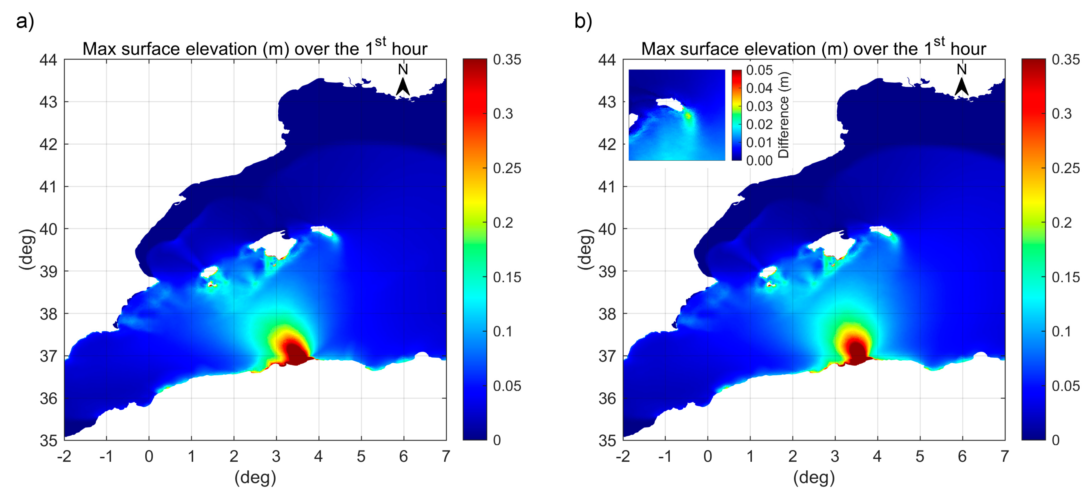
  • simulation of the tsunami effects for a modified version of the fault mechanism originally proposed by Belabbès et al. (2009) [34], considering both a synchronous and asynchronous slip and justifying the need for an increased magnitude passing from seismic to tsunami modeling;
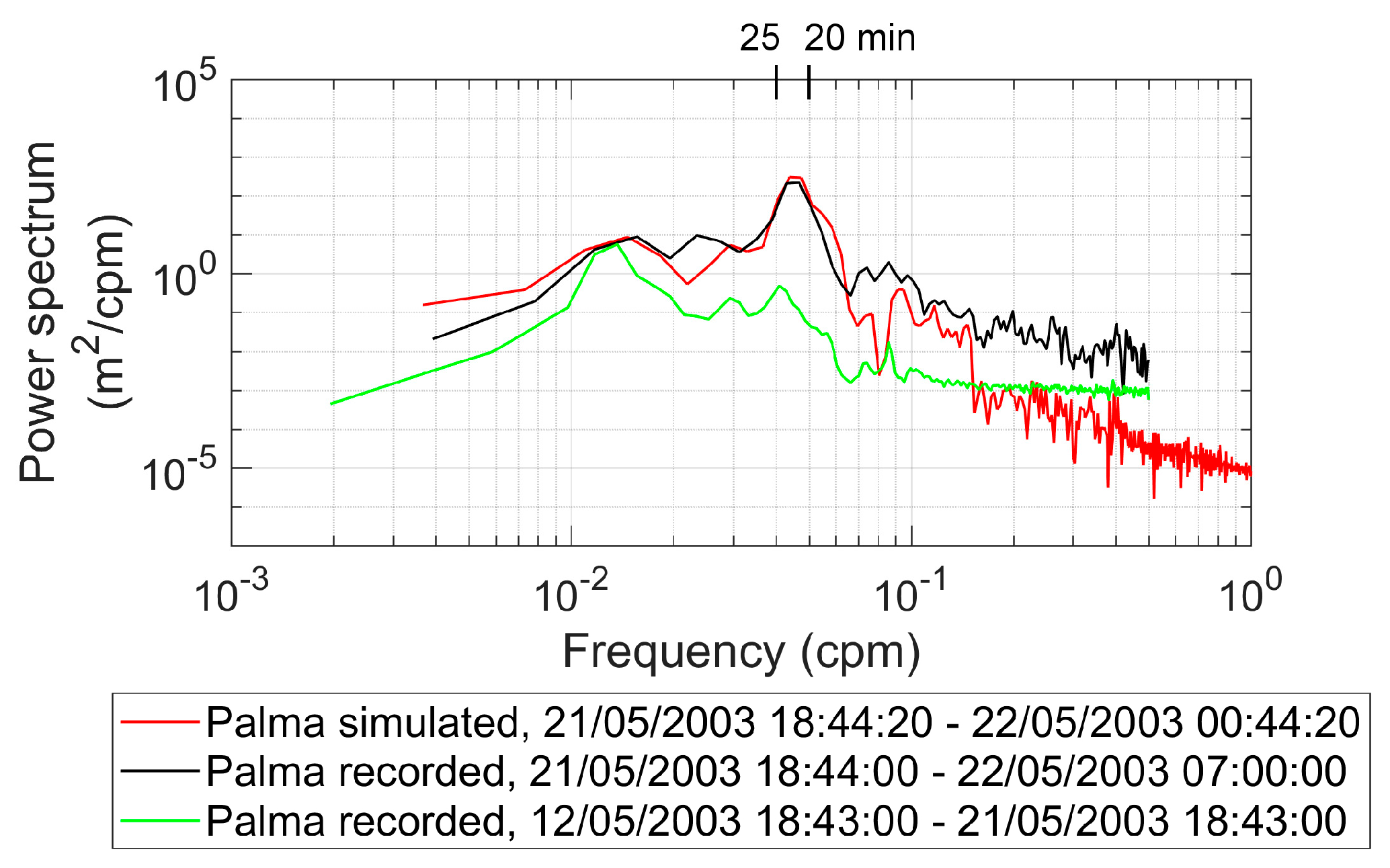
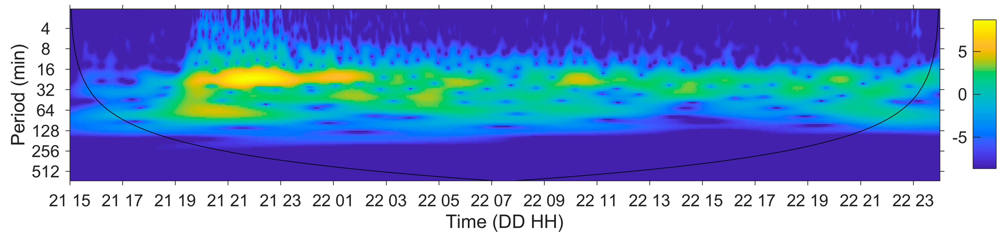
  • highlighting for the analyzed tsunami case the effect of the bay/port resonance in relation to the observed periods and damages;
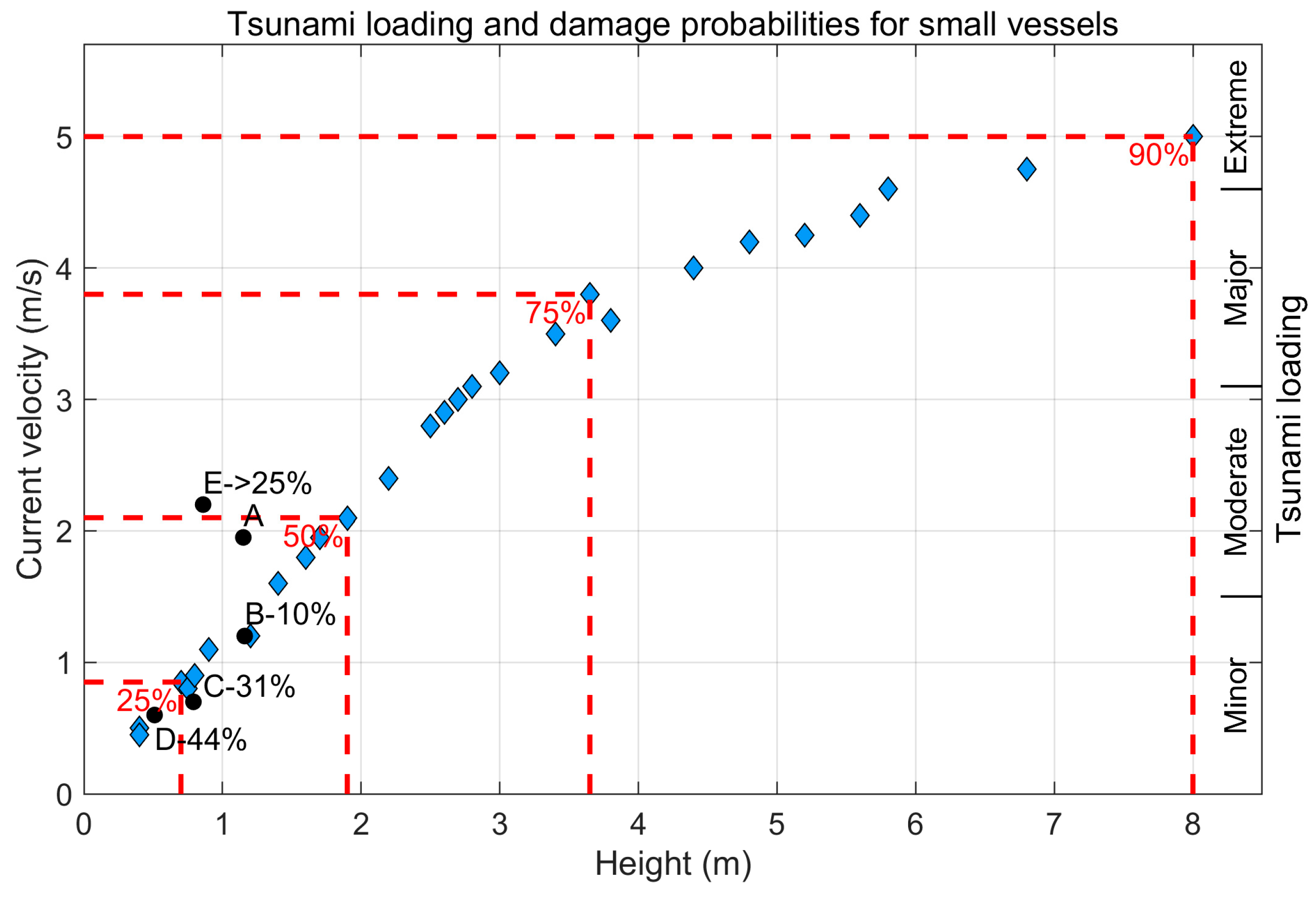
  • analysis of the current intensity and tsunami height thresholds suggested in literature for small ships or boats at berth.

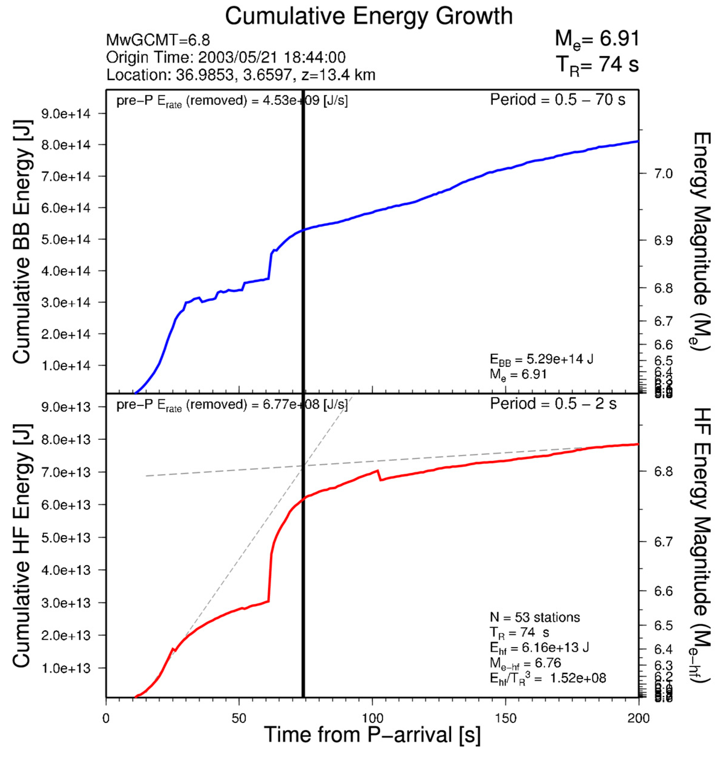
2. Details on the Earthquake and the Tsunami

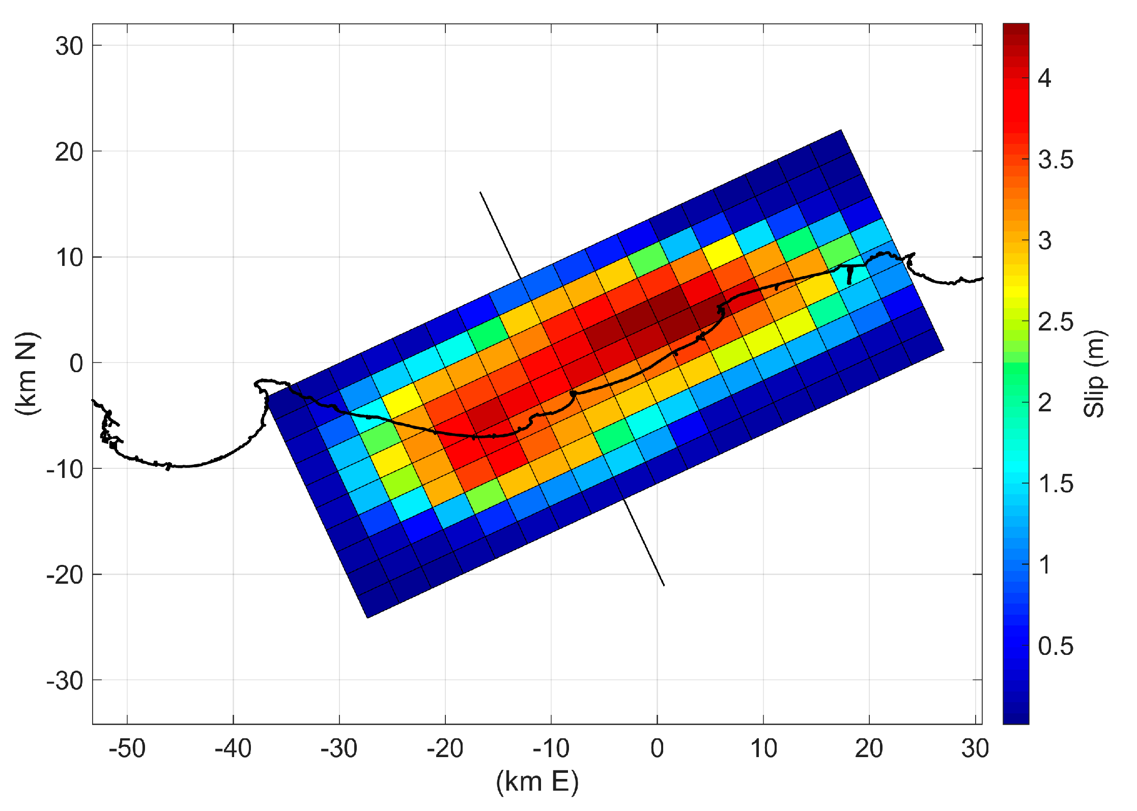
2.1. The Fault Process

The earthquake that struck the northern Algeria on 21 May 2003 exhibited an offshore thrust faulting mechanism mainly related to the compression tectonic regime along the African and Eurasian plate boundary. The present convergence rate between the two plates at the northern Algerian margin ranges from 3 to 6 mm/yr along approximate NW-SE direction [35,36] and is responsible for triggering most of the seismic activity in this region. The 2003 Boumerdès earthquake occurred along the complex thrust and fold system at the northern margin of the Tell Atlas, in the northeastern continuation of the Blida Mountains front and related Quaternary Mitidja Basin [37].
The epicentral area is geologically characterized by a metamorphic basement, mostly constituted by micashistes and quartzites, overlain by Mio-Pliocene and Quaternary clays and sand deposits [38]. The recent Quaternary deposits include the alluvial deposits within the basin and the marine terraces along the coast [21].
Since the mainshock locations obtained by CRAAG, USGS NEIC, and EMSC (Table 2) were in conflict with the measurements of coastal uplift, using a double difference method and three major aftershocks, Bounif et al. [37] relocated the mainshock epicenter on the coastline (3.65° E, 36.83° N) and the hypocenter at 8–10 km depth. The analysis of the aftershock distribution, which extends to about 16 km depth, highlights a NE-SW oriented and south dipping fault and two distinct clusters of seismic events along strike [37].
Several rupture and fault slip models based on teleseismic and geodetic data have been proposed for the 2003 Boumerdès earthquake; some are shown in Table 2.
Most of the proposed models agree on the mainshock hypocenter depth, about 10 km beneath the surface, and on a bilateral rupture propagation from the hypocenter, with two distinct slip peaks. These models indicate a 50–64 km long fault plane, with strike 54–70° (ENE), dip 40–50°, and rake around 90° (thrust mechanism).
A uniform slip distribution of 1.8 m is assumed by Yelles et al. [28] because of the limited amount of available GPS data and spatial coverage. An average fault slip displacement of about 1 m is estimated by Braunmiller and Bernardi [43]. A maximum slip amplitude of about 3 m is estimated west of the hypocenter by Delouis et al. [27] and Semmane et al. [29]; a maximum dislocation of about 2.3 m is found by Yagi [39] 25 km southwest from the hypocenter; maximum slip values of 1.6 and 4.7 m are obtained respectively by Meghraoui et al. [14] and Belabbès et al. (planar model [34]) east of the hypocenter, while a maximum slip of 3.8 m is derived by Santos et al. (solution 1 in [44]) around the hypocenter.
A fault dip change with depth (ramp-flat fault system) is proposed by Déverchère et al. [47,48], by using the data collected during the Maradja cruise in August-September 2003, to explain the two fault scarps identified at the foot of the continental slope ~15–17 km away from the coastline, whose geometry matches in along-strike position, length, and direction the seismic rupture proposed by Delouis et al. [27].
From the analysis of an one-year long aftershocks sequence Kherroubi et al. [49] propose a rupture model strongly controlled by structural heterogeneities and extending as ramp-flat-ramp systems upward, favoring heterogeneous slip and fault segmentation along strike with strong afterslip in the upper part of the rupture.
Also, the examination of the radiated seismic energy determined by IRIS DMC [50] following the procedure described by Convers and Newman [51] highlights that this earthquake exhibits complex and non-instantaneous energy release which is easily identifiable within the cumulative high frequency and broadband energy plots (Figure 1). A rupture duration TR of 74 s is estimated by the fully automated procedure based on the method of Convers and Newman [51]. The earthquake energy exhibits an initial nonlinear growth-period that terminates at about 60 s, followed by a second growing phase which appears to last quite longer. The energy magnitude results 6.91 at the conventional rupture duration but increases (afterslip) exceeding magnitude 7 at 200 s.
A description of the space and time evolution of the rupture process (slip) on the fault plane is given by Delouis et al. [27] and Santos et al. [44], but both restrict the analysis to the first seconds after the mainshock (12 s and 15 s respectively) and therefore do not provide information about the second energy release phase evident in Figure 1.
As it occurred for the 1954 and 1980 El Asnam earthquakes [52,53], also following the 2003 Boumerdès earthquake several submarine telecommunication cables were broken leading to an interruption of the telephonic traffic between Algeria and Europe. An examination of the locations of the submarine cable breakpoints supported evidence of a series of large turbidity currents, triggered almost synchronously and responsible for 29 cable breaks, that occurred from 36 to 228 min after the earthquake at the inner continental slope down to the abyssal plain, over a distance of 150 km along the coast and about 70 km offshore the coastline [54]. However, according to [55], turbidity currents alone are not relevant in tsunami generation because by the time sediment is mixed with water causing density gradient (baroclinic conditions) in the water column, the tsunami has already been generated and is propagating away from the source area.
In addition to the coastal uplift of marine terraces documented in [14] following the 2003 earthquake, an average 100 m seawater withdrawal was observed along 50 km of the Algerian coastline from Corso to Dellys [56]. A seawater retreat was also experienced by the ports of Algiers, Zemmouri and Dellys [57]. Contrary to the mentioned Villebourg event and to the 1856 Djidjelli earthquake, during which the sea retreated about 30–35 m and then returned flooding the Algerian coast [21], the 2003 Boumerdès earthquake did not cause flooding along the Algerian coast but only at the Balearic Islands [26,56].

2.2. The Generated Tsunami

Almost all tide gauges located in harbors facing the Western Mediterranean Sea registered the tsunami waves resulting from the 2003 Boumerdès earthquake (Figure 2, Figure 3, Figure 4, Figure 5 and Figure 6). The largest sea level wave amplitudes were recorded at Sant Antoni and Palma tidal stations on Eivissa and Maiorca Islands, where maximum peak-to-through height of 1.96 m and through-to-peak height of 1.16 m respectively were observed in records (Figure 3). The first tsunami wave arrived at the port of Palma at 19:35 UTC and in Sant Antoni at 19:45 UTC, i.e., 51 and 61 min respectively after the mainshock. Estimation of the first wave arrival time from the Palma and Sant Antoni records, characterized by a good temporal resolution of 1 and 2 min respectively, is more accurate than for all other stations using 5 or 10 min sampling interval. Figure 3, Figure 4, Figure 5 and Figure 6 present the sea level time series at the available tide stations along the Mediterranean coasts after applying a fourth order, phase preserving, high-pass Butterworth filter with 1/3 h−1 cutoff frequency to remove the tidal signal from the original data. In several Spanish harbors the earthquake induced sea level oscillations lasting more than 24 hours (Figure 4). Filtered sea level amplitudes lower than 0.25 m were observed along the French (Figure 5) and Italian coasts (Figure 6).
The Sant Antoni, Ibiza, Palma, Malaga, and Valencia sea level records were examined by Vich and Monserrat [58] through a spectral analysis, identifying a main peak around 21 min and two secondary peaks at 14 and 42 min. The 21 min main period was considered related to the tsunami source.
Through a wavelet analysis using 19 coastal tide gauge records, Heidarzadeh and Satake [59] showed that only the period around 23 min was a powerful signal of tsunami, as it was rather strong in all the examined stations, while other peaks at 14, 30, 45, and 60 min lasted only a short time.

3. Comparison between Hindcasted and Recorded Sea Levels

3.1. The Numerical Model Used

3.1.1. Seabed Displacement

Seven different fault models among those proposed in literature for the 2003 Boumerdès earthquake, inferred from different measurement data (as shown in Table 2), have been used in this study to test their ability in reproducing the observed tsunami characteristics from tide gauge records. The considered earthquake source models are the planar fault models proposed by Yelles et al. (2004) [28], Delouis et al. (2004) [27], Meghraoui et al. (2004) [14], Semmane et al. (2005) [29], Braunmiller and Bernardi (2005) [43], Belabbès et al. (2009) [34], and Santos et al. (2015) [44]. Although some of the indicated source models have already been investigated in other studies (see Section 1.3), they have also been tested by us in order to obtain a comparison independent from the hydrodynamic model effects, as well as to check our implemented geometrical and hydrodynamic model.
The ports of Palma de Mallorca, Sant Antoni, Ibiza, Mahon, Valencia, and Cagliari have been selected to compare modeling results with reported observations. The reasons for this choice have been: (1) the availability of records and information for the Balearic ports, the most affected by the tsunami; (2) the opportunity to examine the long persistence of oscillations at the Valencia tide gauge; and (3) to verify the tsunami effects in an Italian location not directly exposed to the incoming waves as Cagliari. Only two high quality records are available for this event, those of Palma de Mallorca and Sant Antoni; they, however, do not provide adequate azimuthal coverage to estimate a reliable tsunami source model through an inversion method, therefore also other witnesses have been analyzed.
The amount and spatial distribution of slip along the fault plain suggested by Delouis et al. [27], Belabbès et al. [34], and Santos et al. [44] have been obtained processing the corresponding published images, while the Semmane et al. [29] rupture model included in the online SRCMOD database (Earthquake Source Model Database, http://equake-rc.info/SRCMOD/) already in digital format has been adopted. The remaining rupture models have been reconstructed using the information derived from the corresponding references. The fault model proposed by Braunmiller and Bernardi [43] extending to about 3.9°E and composed of two segments with length of about 40 and 10 km has been simplified here by considering a single 50 km long rectangular patch. It is observed that retrieving the slip distribution model on the planar fault from the pixels of the image published in [34] was complicated by the presence of the mesh with triangular elements used by the Authors for modeling geodetic datasets through an inversion procedure to constrain the earthquake rupture parameters. When the image was analyzed the darker trace of the mesh determined along the lines themselves a slip overestimation resulting in an increase of the seismic moment M0 from the value of 1.78 × 10¹⁹ N·m (Mw = 6.8) to 9.10 × 10¹⁹ N·m (Mw ~ 7.2), while retaining the two linked peaks of the pattern indicated by Belabbès et al. [34]. Overestimation was not removed but intentionally maintained in order to represent the fact that energy magnitude had passed level 7 at 200 s. The resulting tsunami period was around 1200 s and slip contributions occurring within a few minutes from the mainshock are naturally accumulated.
For each considered earthquake source model the corresponding spatial distribution of the coseismic surface displacements was calculated from the slip distribution on a 250 m resolution square grid using the Coulomb 3.3 software [60], which implements the Okada analytical expressions for the displacement and strain fields due to a finite rectangular source in a homogeneous, elastic, and isotropic half-space [61]. The seabed deformation process has been deemed to occur instantaneously and the corresponding initial water elevation has been assumed equal to the coseismic displacement of the bottom surface η, determined by the formula
η = H x D x + H y D y + D z
accounting for both the horizontal ( D x , D y ) and vertical ( D z ) components of the bottom displacement vector and the distribution of water depths, H(x,y), in the vicinity of the source [62,63]. This instantaneous water surface elevation has been applied as initial condition for the tsunami propagation model. The seawater depth in the source region of the 21 May 2003 tsunami is in the range from 0 to 1000 m. Considering an average seawater depth of 500 m and a dominant period around 1200 s, a tsunami wavelength of 84 km is estimated. Therefore, since the tsunami wavelength is more than 13 times the water depth at the source, a low-pass filter accounting for attenuation of short wavelength components of the seabed displacement field through the water column, e.g., Kajiura filter [64], was not applied according to [65].
A preliminary test has been carried out to explore the effects of the earth crust mechanical properties, mainly of the Poisson ratio, on the tsunami generation. The source rupture models proposed by Meghraoui et al. [14] and Yelles et al. [28] have been considered and the corresponding vector fields of coseismic sea bottom displacements have been calculated using the Coulomb 3.3 software with different values of the Poisson ratio ν, a constant Young modulus E of 700,000 bar and a friction coefficient of 0.4. The generated displacements have been evaluated and compared in terms of initial maximum surface elevation and drawdown, displaced water volume and potential energy of the initial surface elevation according to the approach described in [62]. Since a reduction of 0.05 in Poisson ratio corresponds to an increase of only 0.01 in moment magnitude, that lies within the overall uncertainty on the Mw estimate, a value 0.20 was finally adopted for ν in all the subsequent computations.
The resulting initial water surface elevation calculated for each of the seven considered rupture models is shown in Figure 7. The maximum uplift of the water surface at the source is obtained with the model derived from that developed by Belabbès et al. [34], 1.86 m, and the minimum, 0.43 m, with the Braunmiller and Bernardi [43] model. The drawdown is rather limited in all cases, ranging from −0.18 m in the Delouis et al. [27] model to −0.04 m in that of Yelles et al. [28]. The maximum values of displaced water volume and potential energy of the initial surface elevation are provided by the modified Belabbès et al. [34] model (4.08 × 10⁸ m3 and 4.20 × 10¹² J), followed by that of Semmane et al. [29] (2.40 × 10⁸ m3 and 1.30 × 10¹² J). The minimum displaced water volume is given by the Meghraoui et al. [14] model and the minimum potential energy of the initial surface elevation by the Santos et al. [44] source (2.57 × 10¹¹ J). Most models present a weak drawdown offshore the fault line and an intense uplift onshore; this explains why at the Balearic coast a very weak depression anticipated the first crest. At the Algerian coast land and water level are raised of the same amount at earth displacement time. In the initial period some flooding is likely due to the difference between the shoreline vertical displacement and the maximum displacement that takes place offshore. This difference has probably activated a minor flooding wave that was probably not observed in the confusion caused by the strong earthquake. The following withdrawal phase, when the shoreline uplift contrasts sea retreat, was certainly much more intense and visible and therefore cited.

3.1.2. Hydrodynamic Model

A fully three-dimensional (3D) model is required for an accurate representation of local large shallow coherent turbulent structures, such as eddies and gyres, generated by tsunamis in the nearshore area or around coastal structures [66,67]. However, for real case studies, a fully 3D model requires a very high computational time and extended memory resources, due to the extensive and complex spatial domain and the very fine resolution needed for tsunami simulation. As no current speed measurements were available inside ports at the time of the 21 May 2003 tsunami allowing the comparison with the simulation results, a depth averaged 2D approach has been applied maintaining reasonable computational time and memory requirements. Models based on the nonlinear shallow water equations are proven to reproduce satisfactorily the current speeds observed during recent tsunami events, e.g., [9,68], and the velocities predicted by these models may be employed for relative comparisons at different locations in a harbor in order to determine potentially damaging currents or to identify particularly vulnerable areas, e.g., [69].
In this study the Hydrodynamic Module (Flow Model FM, release 2012) included in the MIKE 21 package developed by the Danish Hydraulic Institute Water & Environment (DHI) has been used to numerically simulate the tsunami propagation in the Western Mediterranean to the target ports. The flexible mesh (FM) approach adopted by the package is particularly suitable to accurately and efficiently represent complex coastline shapes and allows variable spatial resolution within the computational domain. The package has been extensively used for hydrodynamics and sediment transport modeling in coastal, estuarine, and marine environments [70,71] and has previously been applied in several studies for simulating tsunami propagation [72,73], tsunami runup and inundation [74,75,76,77], to examine tsunami nearshore amplification [78], to investigate resonance response of inlets and ports to tsunami waves [79,80] and for analyzing the nonlinear interaction between tide and tsunami [81].
The modeling system is based on the numerical solution of the 2D nonlinear shallow water equations: the depth integrated Reynolds averaged Navier–Stokes equations for incompressible fluid [82]. The spatial discretization is performed using a cell-centered finite volume method. In the horizontal plane an unstructured grid of triangular elements is used. An explicit scheme is adopted for time integration.

3.1.3. Computational Domain and Unstructured Grids

The hydrodynamic model has been implemented using the unstructured grid and nesting capabilities of the package. A large computational domain covering the entire Western Mediterranean Sea, from the Strait of Gibraltar to the Straits of Sicily and Messina, was used to simulate the tsunami propagation from the source region to the target coastal zones. An area of improved resolution has been embedded in the bathymetry of the large computational domain around the epicentral zone along the Algerian coast, approximately from Bordj El Kiffan to Dellys, extending about 64 km offshore at the longitude of Boumerdès. In this area a mesh refinement with triangular and quadrangular elements has been performed to adequately reproduce the initial surface elevation of the earthquake-generated tsunami.
High resolution local models have also been implemented for the coastal sites of interest, linked to the large model by a one-way offline nesting procedure, i.e., by imposing as boundary conditions for the local model the time series of surface elevation and depth-averaged velocities previously computed by the large model at points along the boundary of the inner domain. The computational mesh of the local models has been progressively refined by scaling the triangular element area in the nearshore zone of the considered target sites where more detail is needed to describe the shoaling effect, the spatial gradients induced by bathymetric features and dynamics within ports.
The computational meshes have been realized by ensuring that the maximum element area was adequately proportional to the local depth (besides proportional to the tsunami wave celerity), and the time step set to a value satisfying the Courant-Friedrich-Lévy (CFL) criterion for an unstructured grid. To provide an indication on the size of the generated meshes, the final unstructured grid covering the entire Western Mediterranean with mesh refinements in correspondence of the earthquake epicentral area, the bay of Palma and the homonym port, used for the simulation of the tsunami generated by the source model derived from that of Belabbès et al. [34], contains 226,076 nodes and 407,703 elements and the one-way offline nested model for the bay of Palma includes 121,252 nodes and 229,056 elements. Similar figures apply to the other grids. The upper limit of mesh element areas in the central Mediterranean Sea, where water depth is around 3000 m and wave celerity is around 170 m/s, was set to 0.00092 deg2 and the minimum angle to 30 deg; the maximum size of an element in this area is therefore approximately 0.030 deg, corresponding to 3370 m. The limit element area was reduced proportionally to water depth and the minimum angle preserved, so that the element size is scaled down proportionally to wave celerity and the average shape is preserved. As illustrative example, Figure 8 shows the progressively refined computational mesh used for the bay of Sant Antoni.

3.1.4. Bathymetry

Bathymetric data for the entire Western Mediterranean have been extracted as XYZ data files from the EMODnet Bathymetry portal (https://portal.emodnet-bathymetry.eu/). A downsampling of the EMODnet data set was necessary to reduce the huge amount of data from the original resolution of 1/8 × 1/8 arc minute to an appropriate point density allowing a practical hydrodynamic model construction at basin scale by using the computational power of an ordinary desktop computer (processor Intel Core i7-6700 with 32 GB installed RAM). In particular, the downsampling procedure has been carried out preserving depth along shallow coastal areas and capturing as much as possible details and morphological features of the sea bottom topography contained in the original data. EMODnet seabed depth is referenced to the lowest astronomical tide (LAT). The effect of the vertical reference of the bathymetric data on the tsunami has been tested.
Since tsunami dynamics in the nearshore zone is significantly affected by local small scale bathymetric features and coastal geomorphological characteristics, very high resolution bathymetric data sets have been constructed for both the tsunami source region and the impacted sites of interest to improve the accuracy and reliability of the numerical models. A wide variety of data sources has been consulted in this study for the construction of the high resolution bathymetric data sets for each considered site. Bathymetric data were obtained by SOCIB (http://gis.socib.es/viewer/, [83]) for the Balearic Islands, by the Autoritat Portuaria de Balears for the Palma de Mallorca port, and were extracted from the MIKE C-Map database for the Southern Sardinia, the Gulf of Cagliari, and the relative port. High spatial resolution bathymetric maps were also compiled using data from the paper nautical charts published in Portolano dei mari d’Italia [84] and by the electronic navigation charts from Navionics (https://webapp.navionics.com) and FlytoMap (https://viewer.flytomap.com/, mainly the raster option). Paper and electronic charts were first georeferenced using QGIS software, then manually digitized and converted in XYZ format. A digitization at very fine scale was carried out to capture the isobaths trend and the depth points plotted on the charts in order to ensure that the local bathymetry was both accurately described and resolved in the models. Careful data inspections and rigorous quality controls have been carried out during the digitization process, excluding water depths deemed to be unrealistic and verifying the values indicated on the charts by cross checking the information contained in the different maps. Further visual checks have been carried out on the final bathymetries resulting from the interpolation performed assigning an appropriate combination of prioritization weights to the various data sets, based on their relative spatial resolution level, in specified subareas of the computational domain.
Coastline shape and position at tsunami time were reproduced with high accuracy for the North Algerian source region and all target sites of interest, including ports that have undergone significant changes in recent years, by manually digitizing from the high resolution historical satellite images available in Google Earth. The digitization accuracy corresponds to the resolution of the used images. For the nested model including the islands of Eivissa and Formentera, in addition to the manually digitized stretches, coastline data obtained from the OpenStreetMap database (http://www.openstreetmap.org) were used. Coastline position data extracted from the Natural Earth website (1:10 million scale, https://www.naturalearthdata.com/) were also used in the basin scale simulation models.

3.1.5. Model Parameters

The simulations performed with MIKE 21 Flow Model FM include the effects of bottom shear stress, eddy viscosity, flooding and drying fronts. The bottom shear stress, τ b ¯ , is determined by a quadratic friction law [82]
τ b ¯ ρ 0 = c f u b ¯ | u b ¯ |
where u b ¯ is the depth-averaged velocity, ρ 0 is the density of the water, and c f is the drag coefficient which can be expressed through the Chezy number, C, or the Manning number, M. Using the Manning number, c f is calculated as
c f = g ( M h 1 / 6 ) 2
where h is the total water depth and g is the gravitational acceleration. The Manning number M is determined by the bed roughness length k S through the relation [82]
M = 25.4 k S 1 / 6 .
It is also observed that the Manning number used by MIKE 21 is the reciprocal of the Manning coefficient, n, given in literature (i.e., M = 1/n). In this study, the bed resistance has been specified through a constant Manning number of 50 m1/3/s applied on the whole domain, corresponding to a roughness length of 0.017 m.
Lateral stresses representing viscous and turbulent momentum transfer and differential advection have been modeled using a sub-grid scale eddy viscosity coefficient given in the Smagorinsky [85] formulation as
A = c S 2 l 2 2 S i j S i j
where c S is a constant, l is a characteristic length scale (characteristic element length), and S i j (i,j = 1,2) is the deformation rate given by
S i j = 1 2 ( u i x j + u j x i ) .
For the Smagorinsky coefficient c S , ranging from 0.25 to 1.0, a constant value of 0.28 has been used in the simulations, allowing sub-grid eddy viscosities between 1.8 × 10⁻⁶ and 1.0 × 10⁸ m2/s.
The flooding and drying scheme of the hydrodynamic model has been enabled in all the simulations to include or exclude in the computations elements/cells that are sometimes wet and sometimes dry, by checking the local water surface elevation. In the present study, flooding, wetting and drying depths have been set to their default values, 0.05, 0.1 and 0.005 m respectively, to avoid numerical instability.
The influence of the Coriolis force has been neglected on tsunami propagation since tsunami frequency band is much greater than the Coriolis coefficient, i.e., the tsunami period is much shorter than a day, e.g., [86].
The coastline has been used as the land boundary. The land boundary is regarded as a closed boundary and the full-slip boundary condition has been applied, that is, only the normal velocity component is set to zero at the boundary. For the open boundaries of the large computational domain located at the Straits of Gibraltar, Sicily and Messina, and for those in correspondence of river outlets or similar features incorporated in all model domains, a Flather condition [87] has been used with external surface elevation and velocity forced to zero. The radiation condition proposed by Flather [87] can be obtained by combining the Sommerfeld condition for the surface elevation η (with phase speed of the surface gravity waves) with a 1D version of the continuity equation applied in the outward normal direction at an open boundary
u ¯ n = u ¯ n e x t g H ( η η e x t )
where u ¯ n is the normal velocity component, H is the local water depth, and u ¯ n e x t and η e x t represent the prescribed external data. In this scheme the differences between the external data ( u ¯ n e x t and η e x t ) and the model predictions ( u ¯ n and η ) are allowed to propagate out of the domain at the speed of the external gravity waves, e.g., [88,89]. The open boundaries have been placed far enough away from the areas of interest so that they do not affect the simulation results. Tidal forcing was not included in the simulations because of the microtidal regime which characterizes the Mediterranean Sea and of the detiding filter applied to tide gauge data.
Due to stability restrictions in explicit schemes, a variable time step interval is used in MIKE calculations and it is determined so that the CFL number is less than a critical value in all computational nodes [82]. To control the time step, a minimum time step of 0.01 s and a maximum time step of 2 s have been considered for the simulations. The CFL number is checked by the procedure to avoid that abnormally small elements may cause instability; the critical value adopted was 0.8, whereas the average value is less than 0.1. The low average value is due to the fact that in ports relatively high water depths are present combined with small scale planimetric elements, as breakwater heads or wharf angles. We have tested different time steps. The 1.5 s time step resulted in no observable difference from 2.0 s, and 3.0 s resulted inconsistent with the critical CFL number.
The higher (second) order numerical scheme has been selected for the time integration and space discretization methods. The higher order scheme is considered in general to produce results significantly more accurate than the lower order scheme, even if its computational time increases by a factor of 3–4 [82]. For the system of 2D shallow water equations an approximate Riemann solver (Roe scheme [90]) is used to calculate the convective fluxes at the interface of the cells [91]. Second-order spatial accuracy is achieved by employing a linear gradient-reconstruction technique. The average gradients are estimated using the approach by Jawahar and Kamath [92]. To avoid numerical oscillations a second-order total variation diminishing (TVD) slope limiter (van Leer limiter [93,94]) is used [91]. The higher order method of time integration uses a second-order Runge Kutta method [91].
A simulation covering 11 prototype hours has been considered for Valencia and 6 hours for the other investigated sites.

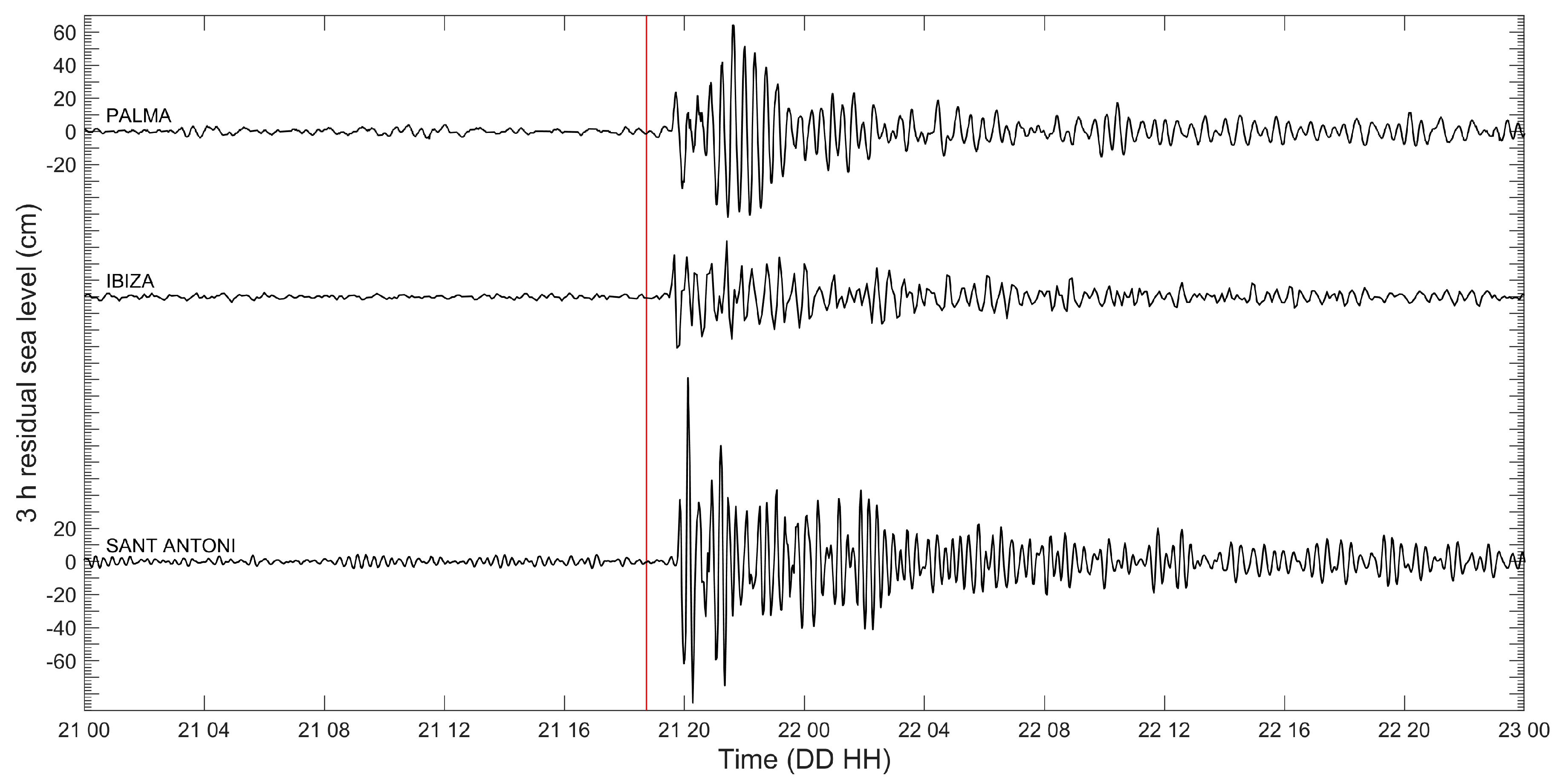
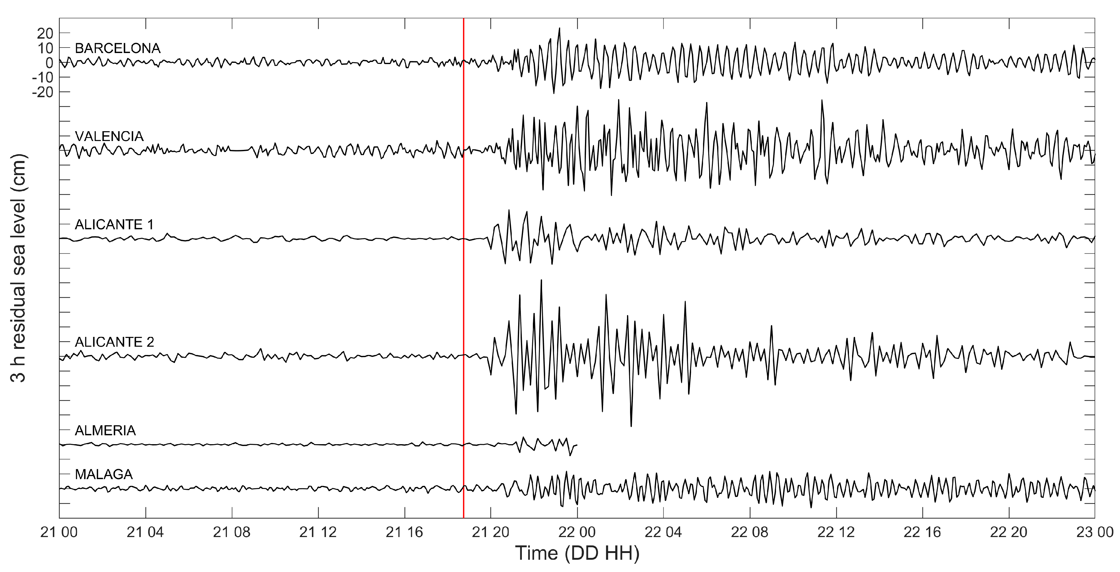
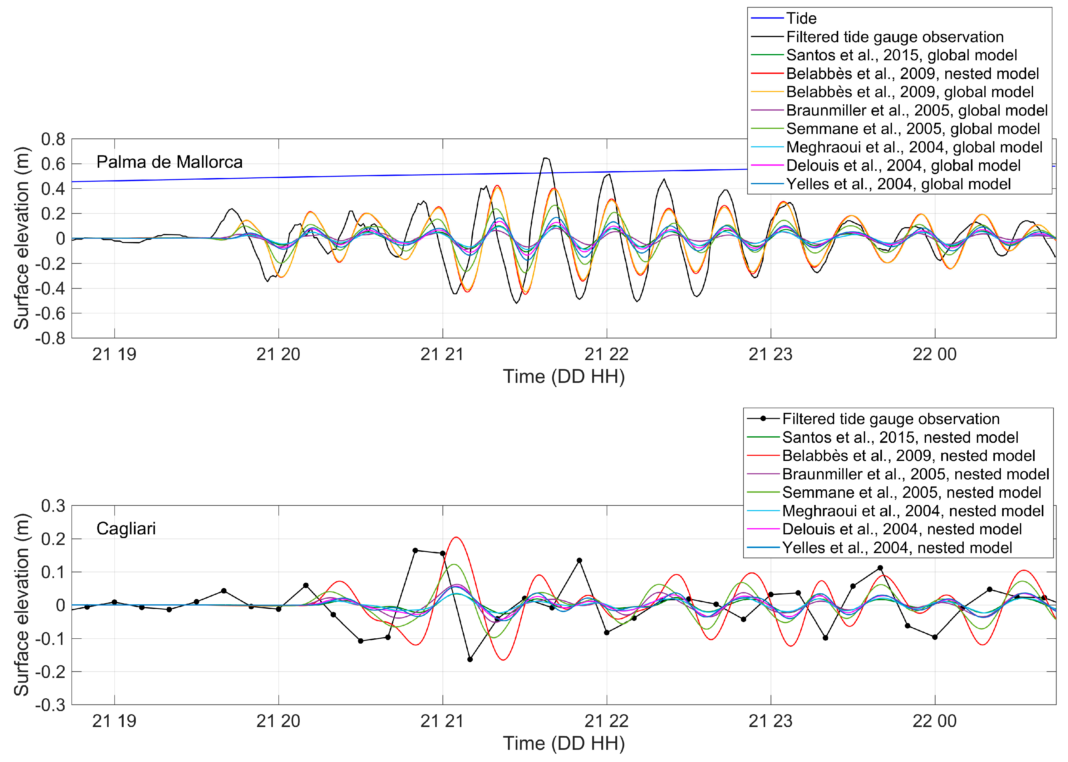
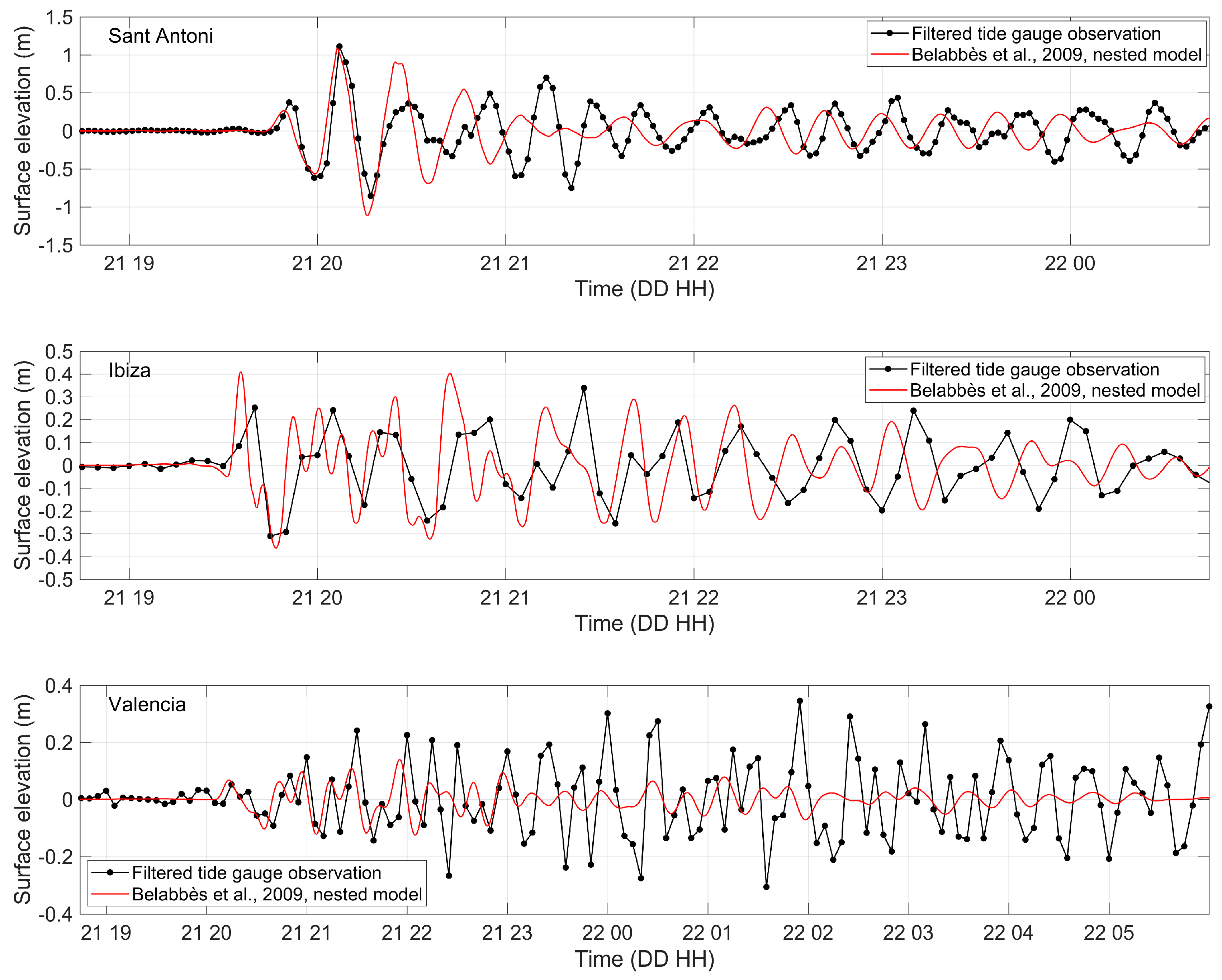
3.2. Comparison between Surface Elevation Results and Tidal Records

In order to check the validity of the implemented mesh, we first compared the results of the simulations representing a simultaneous sliding with available instrumental records. The comparison may be focused on arrival time, tsunami intensity, and mean tsunami wave period, that are respectively dependent on propagation time, seabed uplift/drawdown intensity, and extension of the generation area.
In Figure 9 the tsunami waveforms simulated from the different slip distributions are compared with the detided sea level records at Palma de Mallorca and Cagliari stations. Synthetic event parameters are presented in Table 3.
Among the examined cases, the slip pattern derived from that proposed by Belabbès et al. [34] produces the best agreement between the simulated and the observed waveforms at the considered stations. Therefore, simulations obtained from this slip pattern are compared with detided sea level records at the other stations; the comparison is shown in Figure 10.
A preliminary trivial remark is necessary: the time resolution of tidal records is often not sufficient to represent correctly tsunami waves, containing for this event a dominant component having period around 20 min but also secondary components having around half the mentioned period. Palma station with 1 min record resolution (Figure 9) provides an appropriate description of the real event, Sant Antoni (2 min resolution) a fair one, Ibiza and Valencia (5 min resolution) a poor description, and Cagliari (10 min resolution) an insufficient one.
In Table 3 the arrival time is identified as time of the last zero-crossing before the first evident crest. Extreme levels, root mean square (rms) elevation, and mean zero-crossing period are evaluated over the time interval from tsunami arrival to midnight. Arrival time is affected by a systematic lead error due to time resolution of data; this is irrelevant in numerical simulations but may be important for recorded waves.
In the comparison one must be aware that the first wave including arrival time depends essentially on the generation and propagation model, whereas the following waves depend also on reflection from far shores and resonance of continental shelf waters. It was not possible to describe far coastlines with accuracy similar to that used in representing the Balearic Islands and the target ports.
At Palma de Mallorca tide gauge a 6 min delay in the first perturbation arrival time (19:41:36) is obtained from our simulations, when compared with the detided observations (19:35). Despite the delay, the cross-correlation between the modeled and observed time series of water surface elevation is good; a peak cross-correlation of 0.91 is reached at lag 4.4 min for the first two waves. This discrepancy deserves some comments and analyses.
It must be underlined that a temporal discrepancy of about 6 minutes was also obtained at the Palma de Mallorca tide gauge by Alasset et al. [26] and Vela et al. [32], employing different numerical models and bathymetric data. In the paper by Vela et al. [32] it is stated that a possible explanation “for such an anomaly could be a malfunctioning of the tide gauge’s clock.”
Finally, it should be observed that in the first description of the tsunami event (Díaz del Río, 25 Jun 2003 [95]), then taken up or confirmed by Tel et al. (2004) [96], the arrival time is stated “19:41 GMT”. The article is presented in a newspaper but is written by a scientist and contains a lot of data, all of which are accurate; the article is therefore reliable.
Although tide is almost negligible in the Mediterranean Sea with a spring tidal range of less than 0.25 m [97], a further numerical model was implemented considering a superimposed constant water level of +0.48 m, consistent with the tidal stage at the entrance of the Palma de Mallorca harbor at the tsunami arrival time, to investigate the potential tide influence on the tsunami waves. A reduction of the tsunami arrival delay of only 24 s was found with respect to the tsunami simulation over LAT.
This discrepancy remains an open issue.
The tsunami waveform computed at the location of Sant Antoni tide gauge (Figure 10) results in very close agreement with the recorded signal for the first two waves. The maximum water elevation, 1.11 m occurred at the second wave, is well reproduced by the numerical model. The modeled tsunami arrives slightly earlier, 1 min, than what observed at the tide gauge. The difference is however hardly significant if time resolution of the recorded signal (2 min) is considered.
Tsunami arrival time and height of the first wave predicted at Ibiza and Valencia compare fairly well with the tide gauge data recorded at 5 min interval. The low temporal resolution of the measurements in the port of Valencia does not allow to draw firm conclusions. However, energy reflection from neighbor and distant shorelines documented by any propagation model seems to have great relevance in the Sant Antoni and Valencia ports and/or bays. These phenomena are not well captured by the numerical model, which exhibits relatively rapid dissipation, presumably due to insufficient accuracy in representing distant coastal features. The tsunami waveform at the Sant Antoni and Valencia tide gauges is in fact fairly well reproduced until 21:00–22:00; later wave reflection from Spanish continental coasts and French plus Sardinia coasts, in the order, is certainly superposed on the reflections from the local coasts.
Only for Palma de Mallorca and the fault model derived from that proposed by Belabbès et al. [34] two simulations were carried out: one including the refined description of Palma bay in the global model (multiscale model), and one using results at bay limits as boundary conditions for a one-way nested detailed model of the bay and the harbor. For all the other stations only the nested model was carried out. The analyzed case allows us to point out that differences due to one-way nesting can be assumed as irrelevant for the studied event.

3.3. Comments

The first comment regards the rupture event. Both the time characterization in Figure 1 and the space one in Figure 7 represent a composite event, made up of elementary slip movements occurring in different near locations at different near times. In the numerical model the slip events are represented as occurring simultaneously at 18:44:20.
The second comment regards the effective duration of the movement generating tsunami. Due to the size of the fault zone, generated waves have period of the order of 20 min. Therefore, any congruent movement occurring within a few minutes from the first one did contribute to the tsunami wave.
The classification and conventional characterization of earthquakes is based essentially on the high frequency and short duration characters, as shown and explained in Figure 1, where the conventional duration (74 s) and energy magnitude (6.91) are derived. As far as tsunami is concerned, magnitude must however be evaluated up to a duration of 5–6 minutes, that is out of scale in Figure 1; the estimate 7.2 was obtained by extrapolation following this argument; it remains however an uncertain value, even if also Wang and Liu [24] as well as Gailler et al. [98] find necessary to increase the earthquake magnitude up to this value.
When comparing the offshore tsunami representation obtained by our model with some others available in literature [24,26,30], a more regular distribution of energy during tsunami propagation is visible in our solution. All the used models are based on nonlinear shallow water equations but are different as far as the grid/mesh is concerned. Wang and Liu [24], Alasset et al. [26] and Sahal et al. [30] used a square grid with resolution of 1500, 400, and 1000 m, respectively, in the deep Mediterranean Sea, whereas we have used a flexible mesh having maximum size 3370 m. Despite the grid size differences, quite similar spherical radiation from the source is apparent in [24] and in our simulations, whereas the full front is not visible in the two other mentioned papers. A numerical dispersion effect is possible even if our maximum mesh size is less than 2% of the offshore wave length compared to the DHI suggested limit of 3%. In any case it is recognized that the numerical scheme of MIKE 21 Flexible Mesh appears to be too dispersive to accurately simulate tsunami propagation over large distances [99]. Sahal et al. [30] are not explicit on the representation of bottom friction, whereas Alasset et al. [26] admittedly do not account for it and their model results to be close to stability margin. Conversely, an effect of numerical dispersion of the model we used could be the extreme regularity of the obtained water level pattern.
The space–time evolution of the rupture process may be relevant for the directional distribution of radiated energy. A synchronous movement generates waves mainly radiating in the orthogonal direction to the fault line, whereas coherent space–time shifts along the fault can generate oblique waves as a directional wave maker does. The synchronous slip distribution along the fault plane, modifying the source model proposed by Belabbès et al. [34], is shown in Figure 11. Figure 12a represents the maximum sea surface elevation obtained within the first hour of simulation, i.e., until tsunami wave arrives to Balearic Islands. This pattern is common to all synchronous fault models since the orientation of the different fault planes is similar. Figure 12b shows the effect of a 60 s delay of the eastern slip peak; it is evident the different orientation of the radiation lobe causing intensified effects (~14%) at Menorca Island. A significant increment in terms of maximum surface elevation (~10% within the first four hours after the earthquake) is also estimated over a water depth of approximately 450 m off Îles de Lérins in Golfe de la Napoule (offshore Cannes). Table 4 compares the results of the simulations using synchronous and asynchronous slip along the fault plane at the tide gauge location in Palma de Mallorca and Sant Antoni and at a virtual station in Mahon port and compares them with available observations. The asynchronous slip event results in an increment of ~17% for the first peak elevation at the inner end of Mahon port, while there are no significant sea level variations at Palma and Sant Antoni tide gauges compared to the case of synchronous slip. The arrival time in Palma is however delayed by approximately 1 min, causing further divergence of the model timing from tidal records.
Santos et al. [44] have analyzed the space–time structure of the first 15 s of the seismic event and pointed out two elementary events with relative delay of 6 s and distance 20 km (East first), but the analyzed period is rather short compared to the effective tsunami generation period, containing certainly a further energy release delayed around 60 s.
The space–time structure of the tsunami source remains therefore insufficiently specified. It can justify a systematic delay of the real wave of a few minutes and a deviation of the radiation lobe from the simulated values, causing different intensities at the single Balearic Islands.
In synthesis the asynchronous slip is preferred because it is consistent with time distribution of seismic activity, does not cause evident variation at Palma and Sant Antoni and intensifies the tsunami in the Mahon area where the severest damages were observed.

4. Damages in Bays and Ports Due to the 21 May 2003 Tsunami

As evident from Figure 3 and Figure 12 the tsunami waves severely stroke the Balearic Islands and in particular their bays and ports where refraction and resonance can significantly increase the elevation amplitude and cause strong and unusual currents.
At least 180 boats were totally or partially damaged in harbors and ports of Mallorca, Menorca, and Eivissa, due to the rapid oscillation of the sea water level [100] (Figure 13).
Press reports indicate a total of 73 sunken vessels and about 80 seriously damaged boats only in Menorca Island, e.g., [101] referring to Menorca.info of 23 May 2003 and [102]. The most severe effects of the 21 May 2003 tsunami occurred inside the port of Mahon. In Mahon, it was reported that water disappeared leaving the sea bottom exposed as then returned, flooding the promenade and the road, [101] referring to Menorca.info of 22 May 2003. The Colàrsega and Port d’Hivernada, situated at the internal end of the Mahon port, experienced the greatest damage. Drifting yachts, sunken fishing boats, overturned boats, and fishes on the asphalt could be seen. Only in Colàrsega 11 sunken vessels and 26 damaged were counted; furthermore, in the area there were three sunken floating docks and serious damage to the dike closing the harbor [101]. It was reported that at Cala Llonga 20 vessels sank [101] and a pier was destroyed [103], and in the rest of the Mahon port, there were two sunken and two damaged vessels [101].
Press reports also indicate significant damage at Cala de Sant Esteve where some houses located near the sea were flooded and medium-size vessels suffered the effects of the sudden change in the sea level and ended up on the ground [101]. Roig-Munar et al. [104] show an impressive photo with boats accumulated at the end of the Cala de Sant Esteve embayment (Figure 13b).
At Mallorca the most relevant effects of the Boumerdès earthquake were observed along the northern and eastern coasts of the island, at Pollensa and Alcudia [105], in Andraxt port and at the south extreme [100]. Information regarding the impact of the 21 May 2003 tsunami in the port of Palma de Mallorca indicates that:
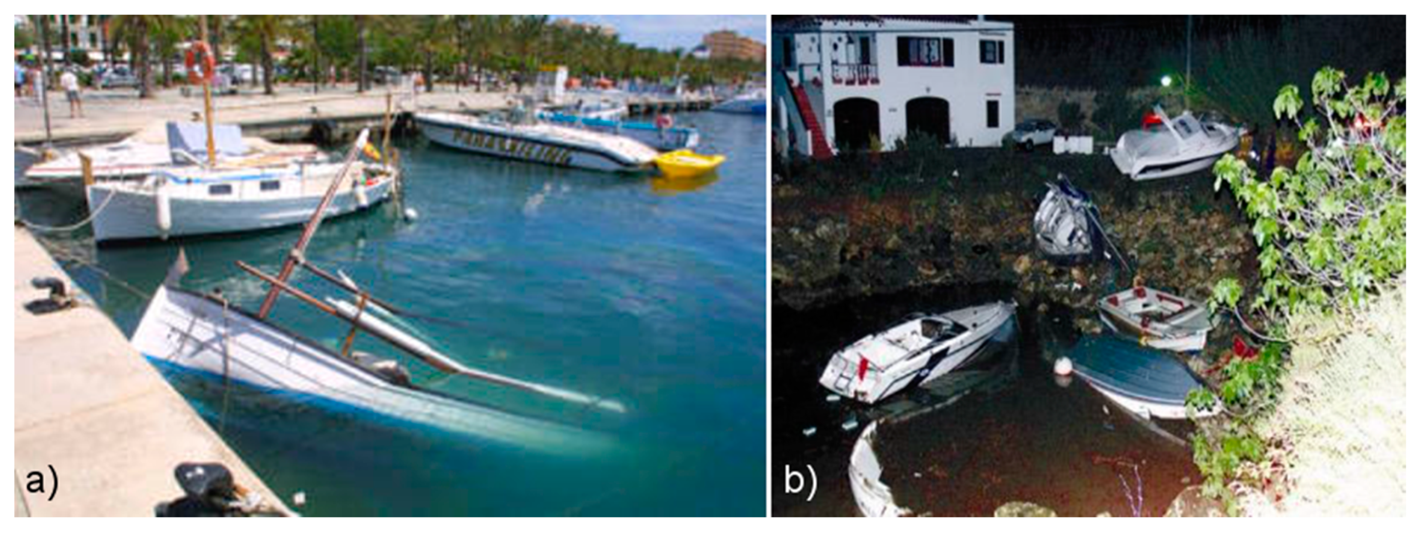
  • “the damages generated by the 2003 Western Mediterranean tsunami in the Palma harbour concentrated in the northern basin where several pleasure and sailing boats sank between Sant Magí dock and the Royal Yacht Club. The shallow water depth in this part of the harbour eased the sinking of the boats, as they were quickly moved up and down by the oscillations easily hitting the bottom and breaking” [31];
  • the boats moored along the Paseo Maritimo close to La Riera hit the bottom due to the rapid lowering of the sea level [105];
  • collisions among vessels occurred along the Paseo Maritimo [103];
  • “in Palma, the first sea movement was an ingression and the Paseo Maritimo street was flooded” [106];
  • “a second highly impacted area was the Espigón Consigna, in the commercial quays, where the tsunami waves took off an oil container and other objects” [31].
In Eivissa, following the Boumerdès 2003 earthquake, several coastal areas were flooded, mainly the bay of Sant Antoni de Portmany and Santa Eulària [105].
Along the Sant Antoni coast, the water withdrew about a hundred meters letting see the sea bottom, and then returned in the form of a great wave, which flooded an extensive part of the promenade and made to collide boats which were moored in the port. As a result, several boats sank, others ended up on the piers and crashing against the cars parked nearby [105]. The port parking and the fishermen’s pier were among the most affected by the tsunami [107]. About fifteen boats were damaged in the port of Sant Antoni [108]. Various vehicles that were parked along the promenade were also damaged due to the sea level rise [103,109].
In Santa Eulària harbor a wave of 1.5 m swept the piers and at least two boats, among which a 15 m yacht, sank [105]. At Ibiza, a tugboat sank in Marina Botafoch and deteriorated moorings were found in Ibiza Nueva [108].
Regarding the French Mediterranean coasts, the results of a three-month field survey started on May 2007 to look for potential witnesses of the tsunami induced by the Boumerdès earthquake showed that in only 8 harbors of the 135 investigated hydrological anomalies were noticed during the evening and the night of 21–22 May [30]. In particular, in the harbor of La Figueirette, where some boats were damaged, the water level lowered about 1.5 m and eddies, boiling phenomena, and strong currents up to “15 knots” (7 m/s) would have been observed. A sea level drop of about 1.5 m and a maximum current of “12 knots” (6 m/s) would also have been observed in the harbor of Cannes‒Vieux-Port, along with numerous 2 ton moorings moved [30].
In Antibes strong sea waves were signaled by yachtmen, while a sea retreat of 1 m was observed near Hyeres [110].
No damages were reported in Italian ports.

5. Relating Tsunami Hydrodynamic Features to Reported Damage

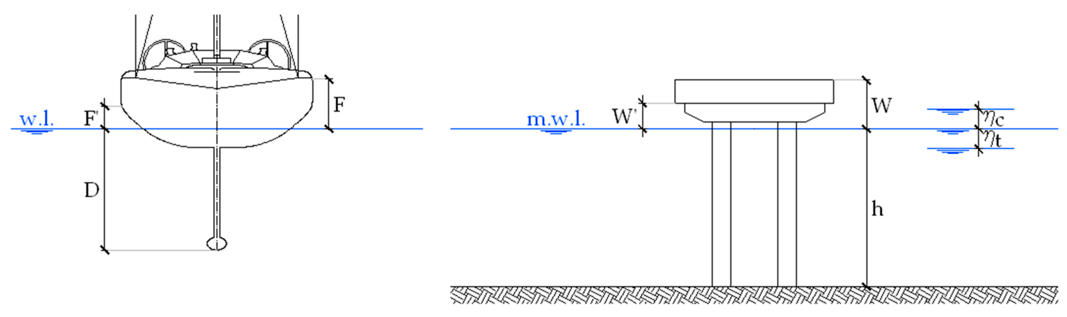
5.1. Tsunami Loading Factors

Recent tsunami events originating off the western coast of Sumatra on 26 December 2004, off the Maule coast of central Chile on 27 February 2010 and off Japanese Tohoku coast on 11 March 2011 generated a series of tsunami waves with devastating effects not only along the coast of their respective source regions but also in far field coastal areas. Pertinent information about the tsunami events were collected by several field surveys using established protocols, questionnaires, and interviews. Strong tsunami-induced currents, documented by eyewitness accounts and available instrumental and video records, e.g., [113], have been identified as responsible for most of the damage to boats and docks in a number of ports and harbors at different locations following these events [114,115,116,117,118].
Numerical simulations of the currents induced by the 2004 and 2011 tsunamis in selected harbors were performed by Lynett et al. [66], showing that, during tsunami events, damaging currents are driven by coastal-structure induced or topographically controlled water jets, large eddies, or 2D turbulent coherent structures. These large shallow water coherent structures can greatly increase the drag force on the affected infrastructure and the ability of the flow to transport debris and floating objects [119].
A simple relationship between simulated tsunami currents and observed damage was proposed by Lynett et al. [9] for small craft harbors by using the information relative to the impact of the 2010 Chile and 2011 Japan tsunamis on the California coast documented by Wilson et al. [117] and additional observations provided by Lynett et al. [66,120] and Borrero et al. [121]. Damage to floating docks and vessels in harbors initiates with current speeds of approximately 3 knots (1.5 m/s). When the current speed threshold of 6 knots (3.1 m/s) is exceeded, damage transitions from moderate to major. Extreme damage occurs when current speeds exceed 9 knots (4.6 m/s). The indicated thresholds are subjected to uncertainties affecting both the load-carrying capacity of structural components, which is highly dependent on their age and deterioration level, as well as the current predictions which are particularly sensitive to bathymetry and numerical errors [119].
Also, sudden and significant water level fluctuations can lead to various hazards inside the harbors. Wilson and Miller [122] propose the FASTER approach to determine during a tsunami alert the maximum water elevation that the tsunami could reach at a particular coastal location.
Suppasri et al. [123] examined data for approximately 20,000 small vessels damaged during the 2011 Tohoku tsunami. The damage data were analyzed against the peak tsunami heights observed from field survey and the peak flow velocities obtained from numerical simulations using nonlinear shallow water equations.
Four major types of damage to vessels caused by tsunami were considered: (1) grounding, that is the impact of a boat on seabed when the water level falls during the receding tsunami wave; (2) stranding, occurring when the elevation of the vessel bottom is raised higher than the pier elevation in a harbor; (3) failure of mooring rope; (4) loss of stability, i.e., overturning and loss of its tendency to return to an upright position.
Loss functions for tsunami damage to vessels were developed by Suppasri et al. [123]; cases were classified based on the vessel tonnage, motor type, and distance from the tsunami source (representing the possibility to escape the most dangerous conditions).
Muhari et al. [124] developed a 3D loss estimation surface to represent the damage probability of vessels associated with tsunami parameters and boat characteristics, including the effects of collision experienced by vessels during the tsunami. The surveyed loss data of vessels previously employed by Suppasri et al. [123] were used by Muhari et al. [124], but only vessels anchored or moored in the port before the tsunami were considered in this paper to reduce uncertainty of the selected vessel data. Tsunami heights and speeds were simulated using the shallow water approximation and a nested grid system with smallest domains having 10 m grid resolution.
In the following, in the absence of observed current data during the 21 May 2003 tsunami event, the results of the Flow Model employing the asynchronous slip distribution, modified from the source model proposed by Belabbès et al. [34], have been used to establish the role of tsunami-induced currents and sea surface elevations in causing observed damage inside the ports of Palma de Mallorca, Sant Antoni de Portmany, and Mahon in the Balearic Islands.
Tsunami oscillation in harbors and bays where extremes are reached is frequently affected by resonance [30] that may also affect the peak period of oscillations and time of internal oscillation set up. Therefore, while examining response of different harbors, the proper oscillation periods are identified as peaks of the response spectrum to a broad band forcing that occurs in good weather/background conditions [125].
Several site names appear in the text; the reader can see the corresponding positions by searching the name in some web mapping tools (as Google Earth or the chart viewer https://webapp.navionics.com).

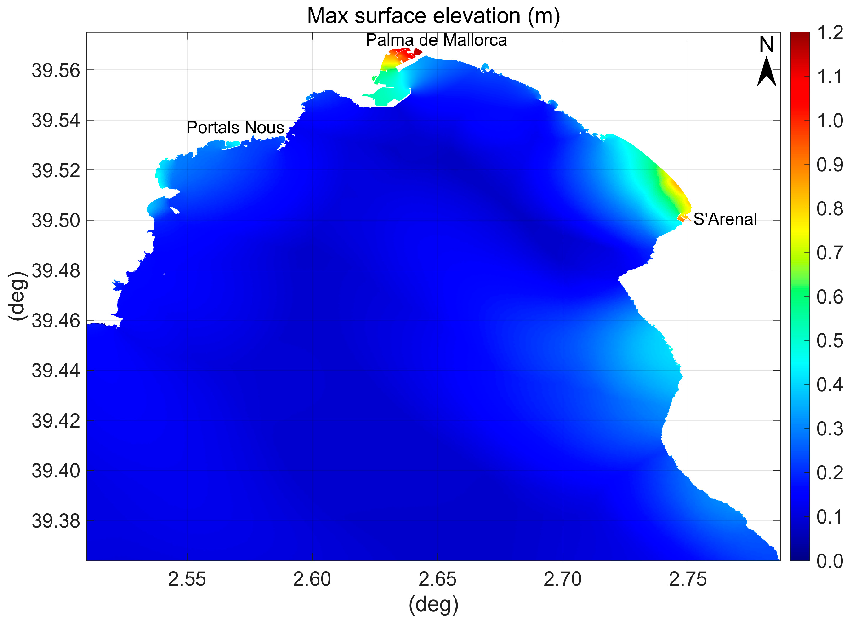
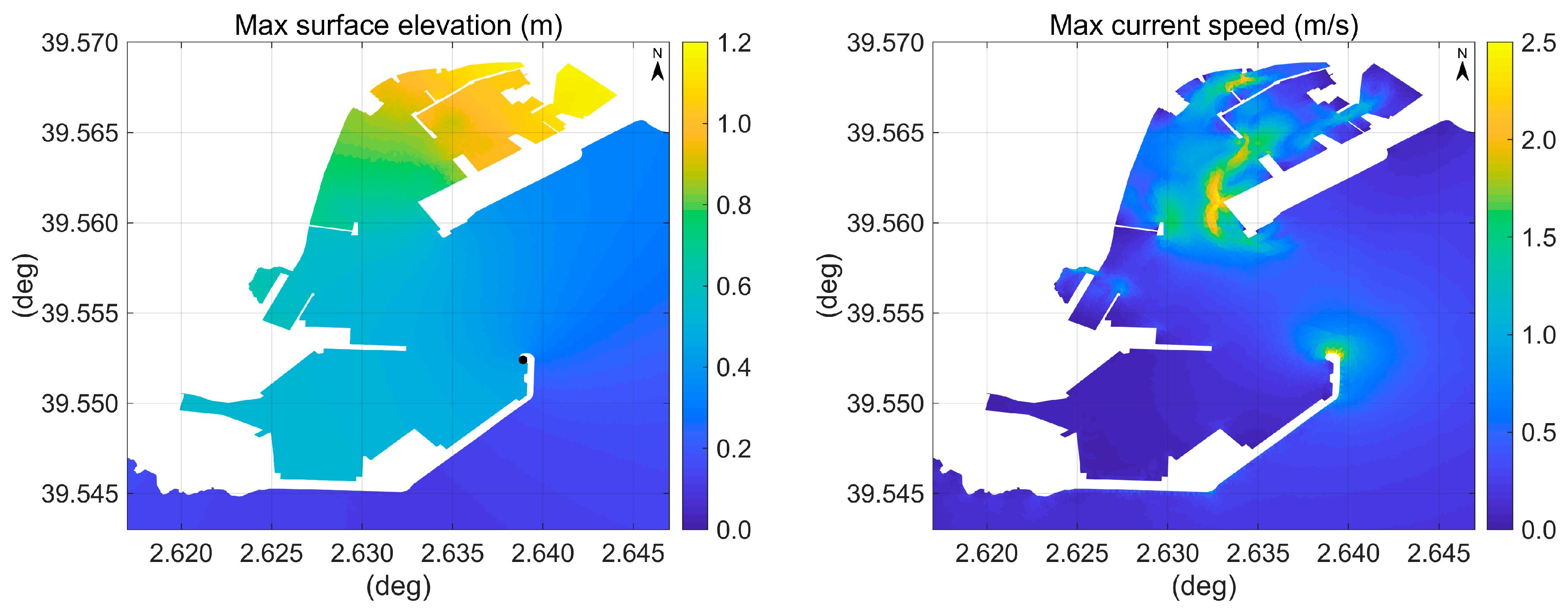
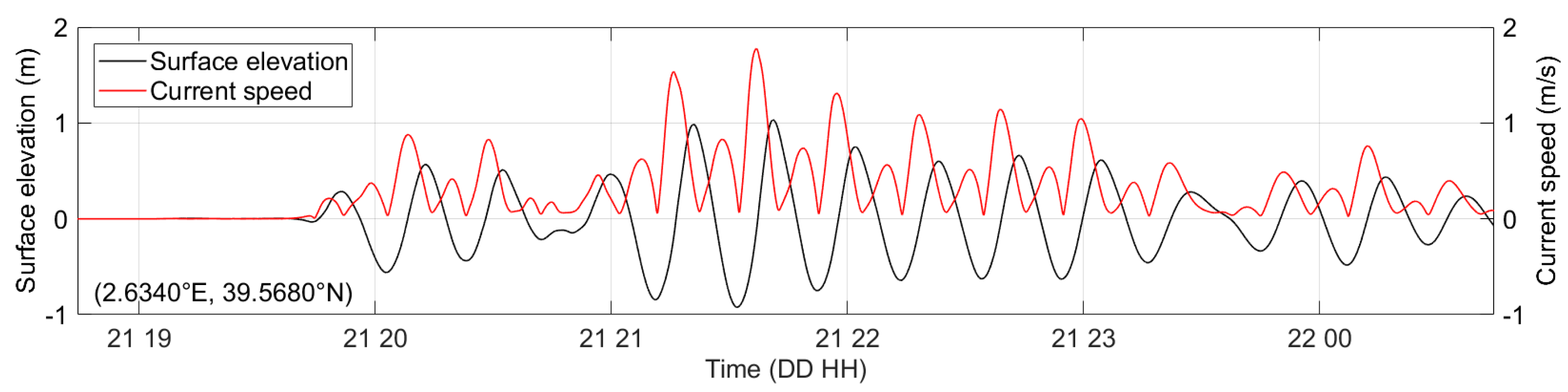
5.2. Port of Palma de Mallorca

The spatial distribution of the maximum water surface elevations obtained in the Palma bay and port over the 6 h tsunami simulation is shown in Figure 14 and in the left plot of Figure 15, respectively.
The highest water surface elevations are observed in the northernmost corner of the Palma port near La Riera and in the northernmost end of the ancient harbor, where the wave height reaches 1.15 m over the current mean sea level (+0.48 m over LAT). The maximum water drawdown, −1.07 m, is also observed in these same areas within the port. The maximum tsunami-induced depth-averaged current speeds calculated over the 6 h tsunami simulation are displayed in the right plot of Figure 15. The highest current speeds occur at the head of the West Breakwater, ~3.2 m/s, and at the head of the commercial quays, ~2.3 m/s. It is specified that the maritime infrastructures represented in the figures are interpreted as impermeable. As fixed piers supported by piles are not easily recognizable on Google Earth images, current speed peaks at their head might be not such intense as indicated. Figure 15 shows, however, that where the current intensity exceeds 1.5 m/s and moored boats may be present, damage to boats has been observed. The modeling results also indicate that the tsunami current direction is transverse with respect to the boats moored at the Sant Magí and adjacent marina docks. In this specific location inside the port the boats are moored to dock at a perpendicular angle using a Mediterranean style mooring. Due to the large unexpected sea level oscillations, this mooring style may have favored vessel collisions. Computed time histories of water surface elevation and current speed during the tsunami at a virtual station located between the Sant Magí dock and the Royal Yacht Club, where most of the damage occurred, at a depth of ~1.7 m, are shown in Figure 16. The numerical results highlight that the highest current speeds occur during the rising water level.
Significant current speeds of ~1 m/s are also detected at the end of the westernmost floating dock of the Palma’s Royal Yacht Club due to the narrow passage and at the head of the Espigón Consigna, the easternmost jetty in the commercial quays area, combined with, in this last case, a water surface elevation up to 1.13 m.
The simulation results also show that the flow is affected by rotational eddies of moderate strength forming at the head or at the sides of the jetties and docks.
In agreement with Vela et al. [31], tsunami wave amplification also occurred in Palma de Mallorca due to resonance effects. A spectral analysis of the observations has been performed to evaluate the frequency content of the sea level oscillations recorded at the tide gauge and to examine the influence of the tsunami source characteristics and resonant properties of the site. The background spectrum was evaluated considering the data of a long time interval preceding the tsunami event, from 12 May 18:43 to 21 May 18:43 that mainly reflects the normal good weather conditions with no single prominent excitation source, so that it highlights with greater reliability the topobathymetric resonant characteristics of the measurement site. The tsunami spectrum was determined for the time series covering the event, from 21 May 18:44 (earthquake occurrence time) to 22 May 07:00. Both time series have been previously detided; the power spectra of the residual time series have been then calculated through the Welch method using a Hamming window with 50% overlap; the computed tsunami and background spectra are shown in Figure 17.
The background spectrum has prominent peaks at periods of 11.6, 24.4, and 73 min (and secondary peaks at 13.5 and 34 min); these spectral peaks are associated with the natural oscillation modes of the bay system including the port. The 73 min period corresponds to the fundamental (Helmholtz) mode of the inner bay, from the shoreline down to 50 m water depth at the entrance of the bay, between Cap de Cala Figuera and Cap de Regana. 24.4 min, being around 1/3 of the previous one, represents the period of the second oscillation mode of the bay.
The tsunami energy spectrum has a peak corresponding to a period in the interval 21–24 min. Analyses of the May 2003 tsunami performed for several coastal stations in the Mediterranean basin by Vich and Monserrat [58] and Heidarzadeh and Satake [59] arrive to the conclusion that the source spectrum has a peak around 21–22 min. This peak is however close to the prominent natural period of 24.4 min identified in the Palma background spectrum and suggests a pronounced influence of resonance on the long wave oscillations at this site, with a shift of the peak toward greater and more amplified periods. The slow time-growth of the mode amplitude suggests a weak interaction between the long-lasting tsunami waves and the oscillation mode.
The results of a wavelet analysis using a Morlet mother function, applying the procedure described in [126] to the Palma tide gauge record, also reveal the temporal variations in the dominant period of the sea level oscillations (Figure 18). In Figure 17 the power spectrum of the time series obtained at the tide gauge location from the simulation is also shown. Considering the frequency resolution obtainable from the 6 h modeled time series, its spectral peaks compare well with those of the longer tide gauge series.
The observed maximum water levels appear therefore to be related to a mechanism of tsunami wave amplification associated with resonant excitation of natural modes of the bay. A NW-SE nodal line orthogonal to the major axis of the bay is clearly distinguishable in Figure 14 as characterized by lower sea surface oscillations. Figure 14 shows also two elevated water levels in the opposite corners of the bay, at the port and at S’Arenal. They represent transversal oscillations in the bay that were already recognized by Vela et al. [32]. They have periods ranging from 5 to 10 min and are immediately triggered upon arrival of tsunami wave, but fade much more rapidly than longitudinal ones (Figure 3 and Figure 18).

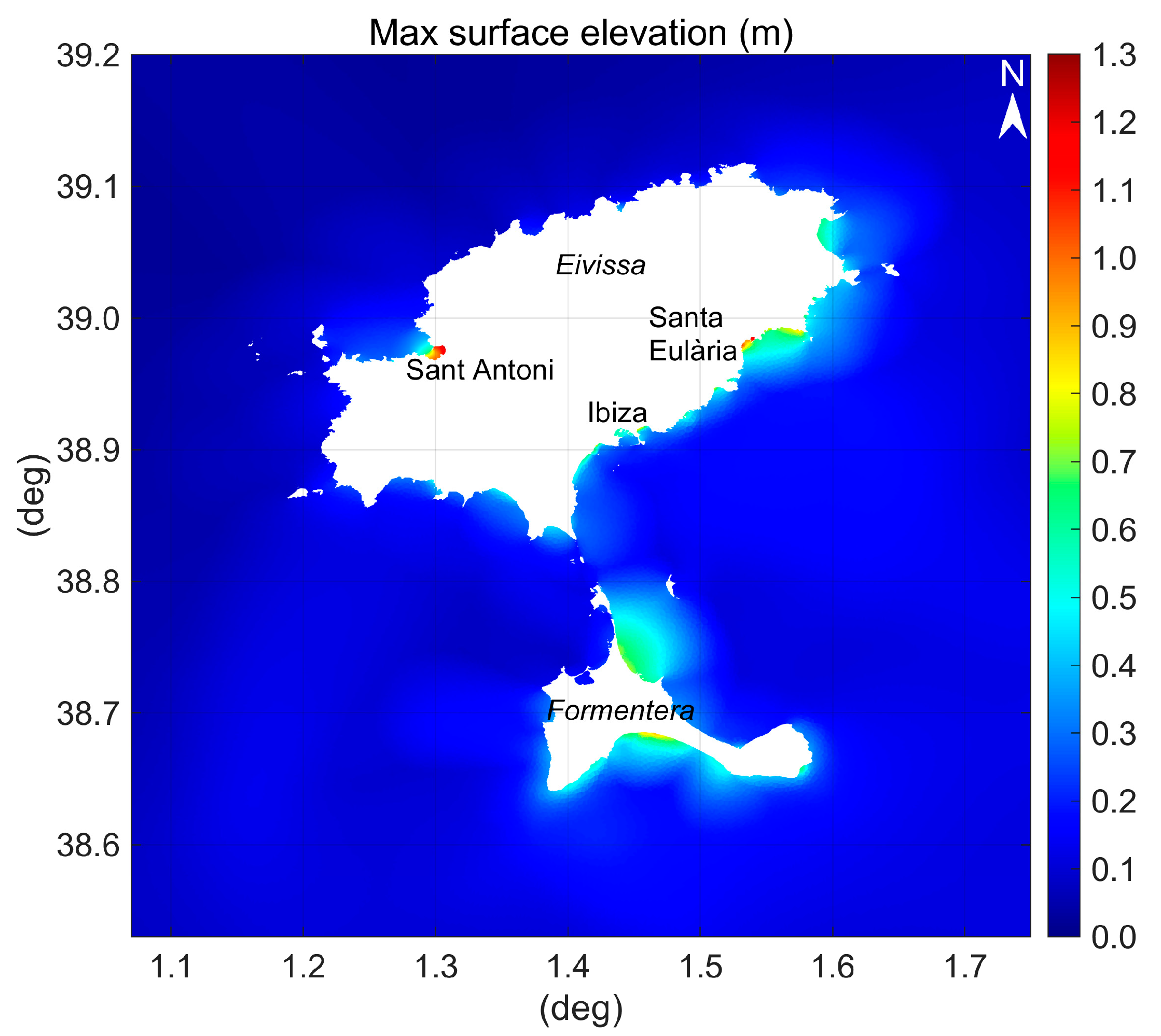
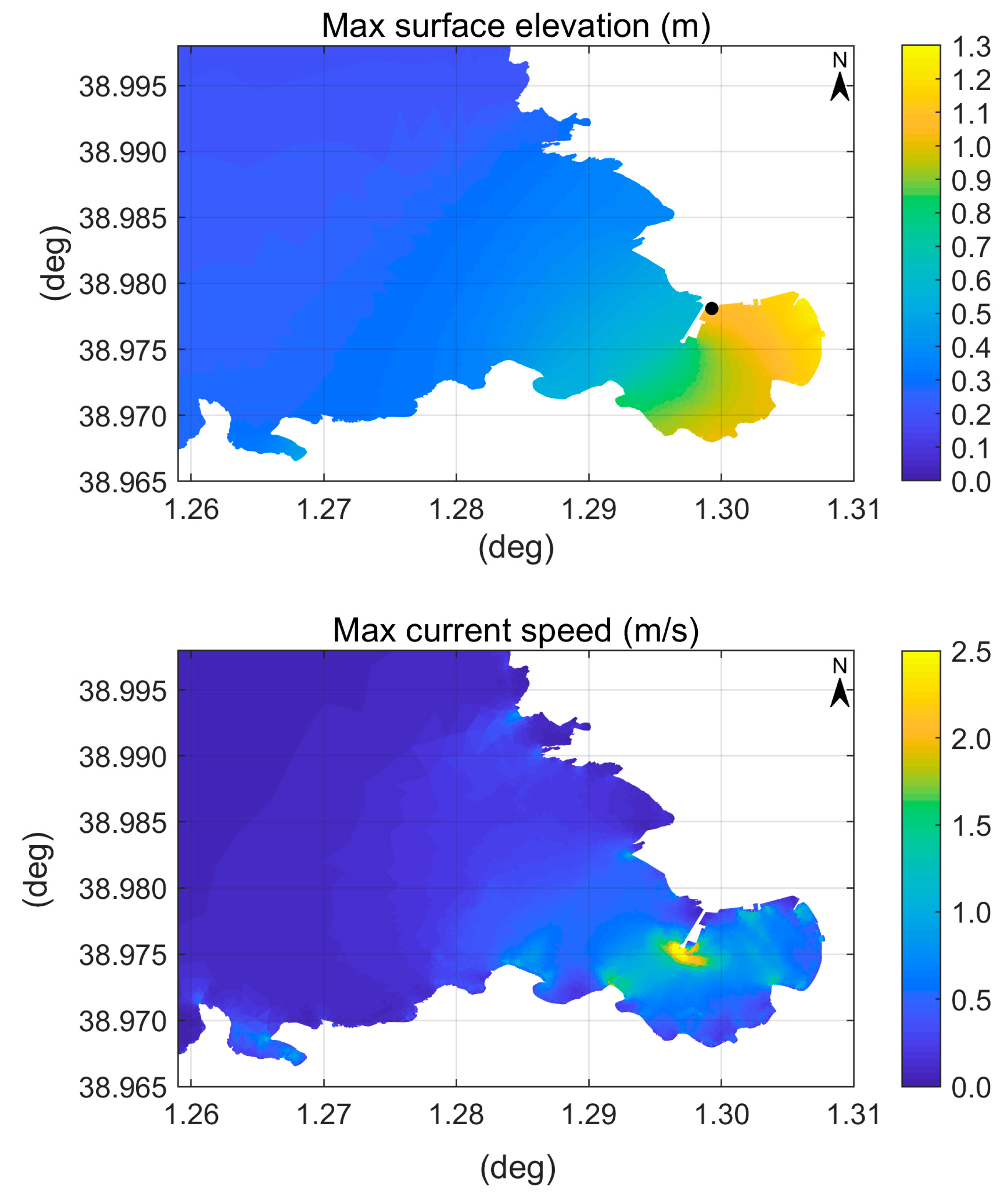
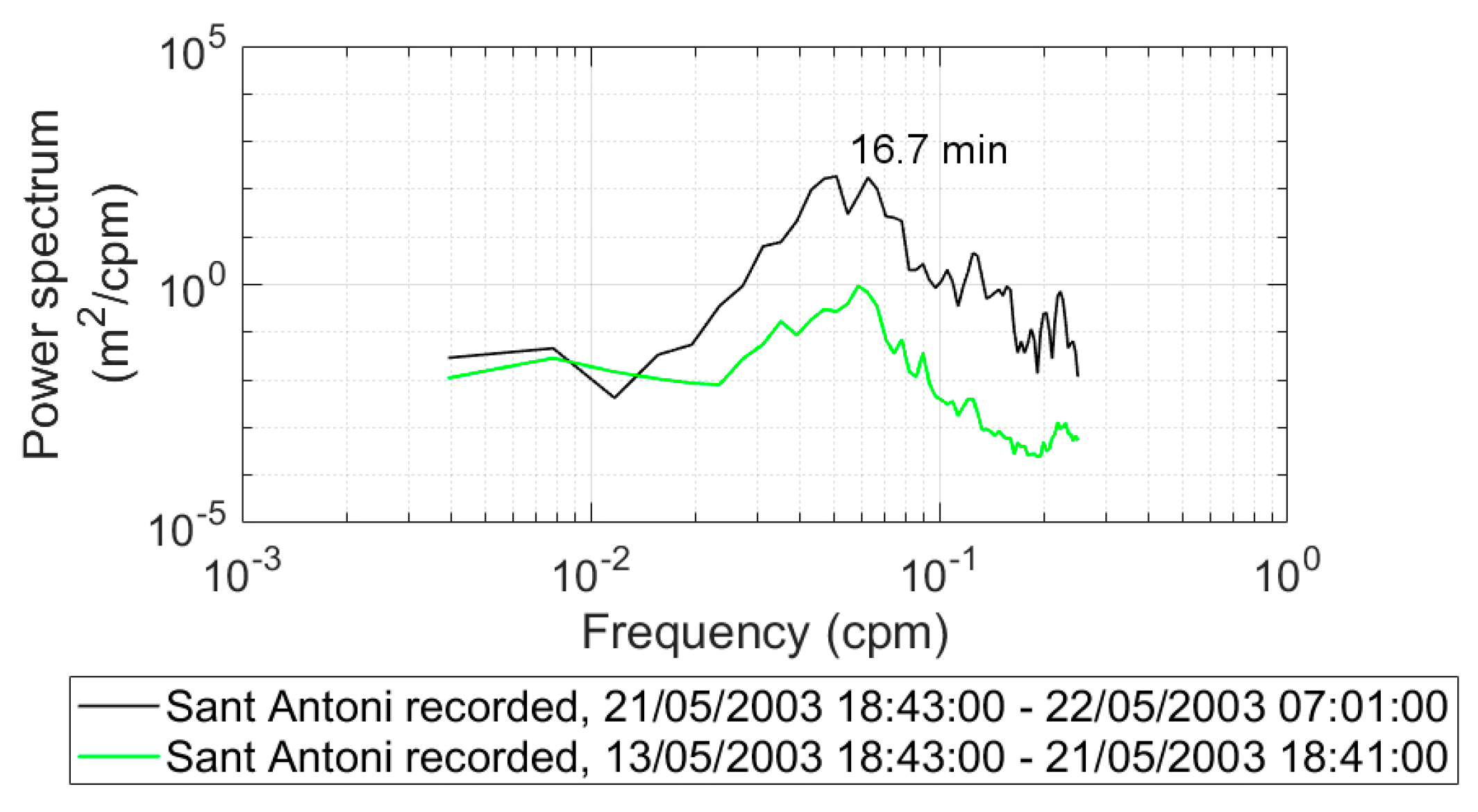
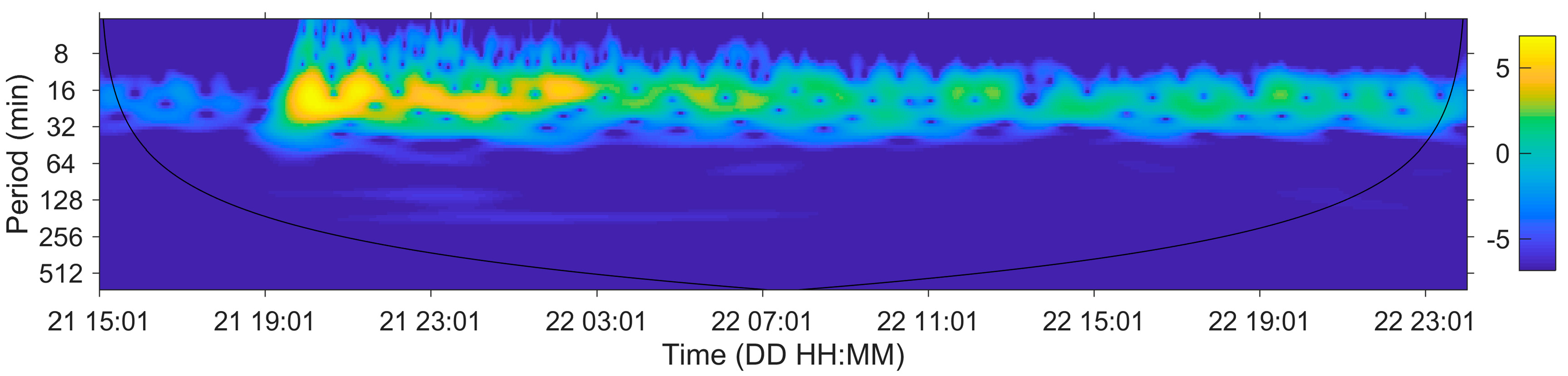
5.3. Port of Sant Antoni de Portmany
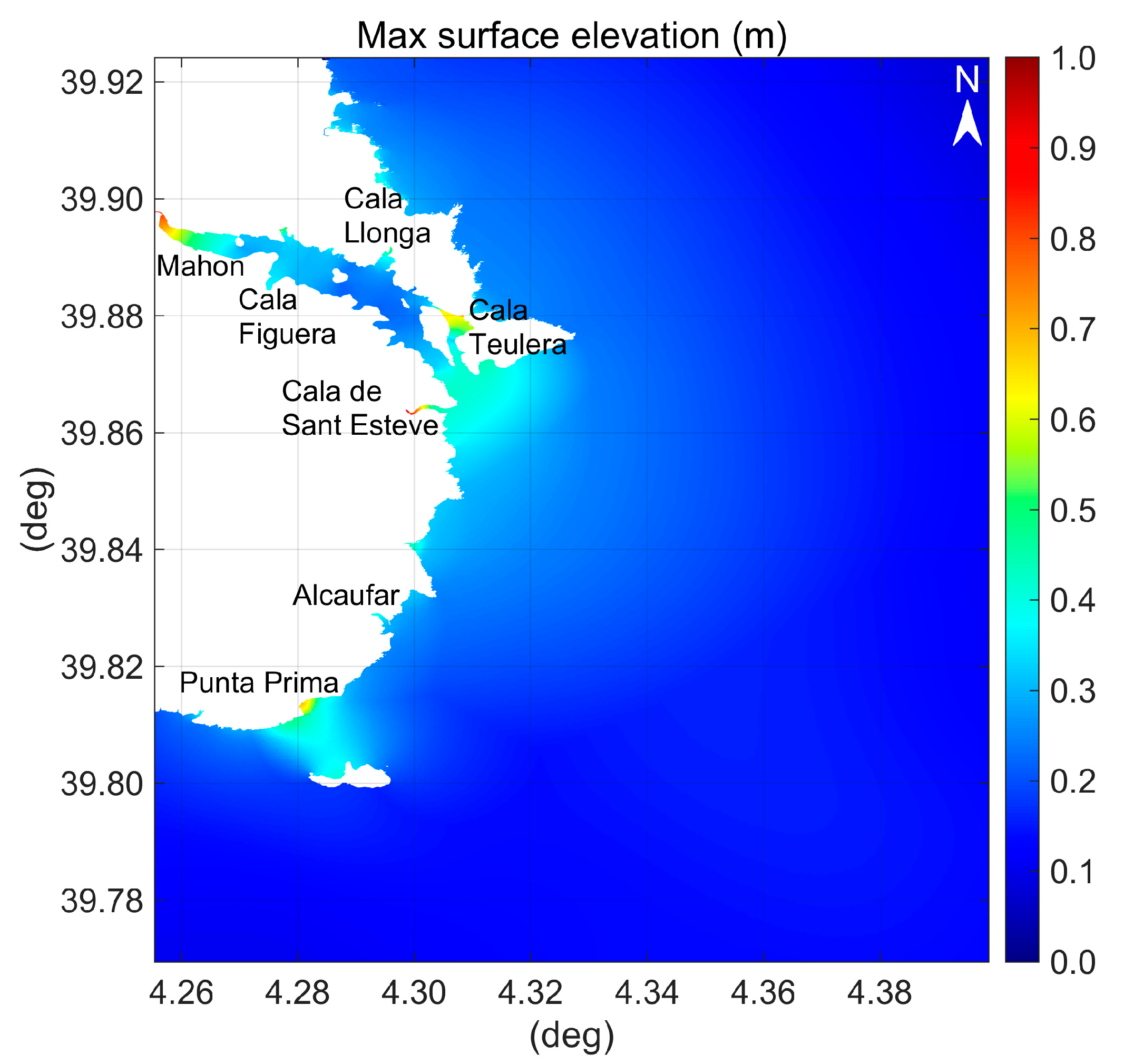
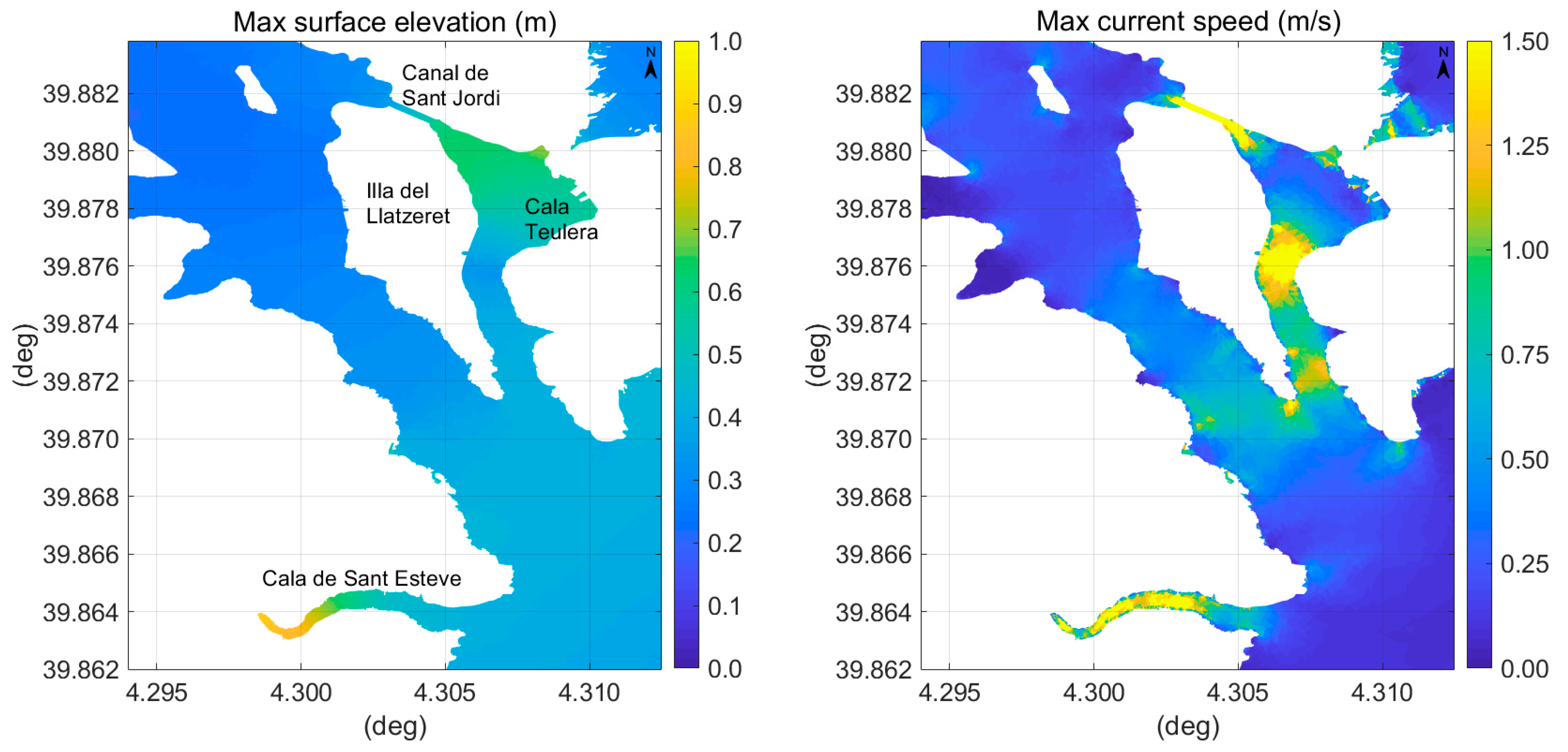
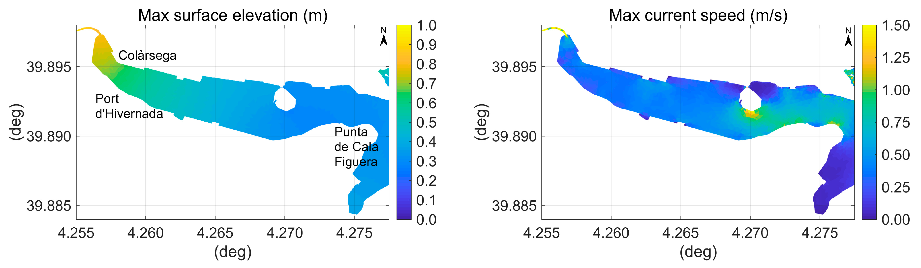
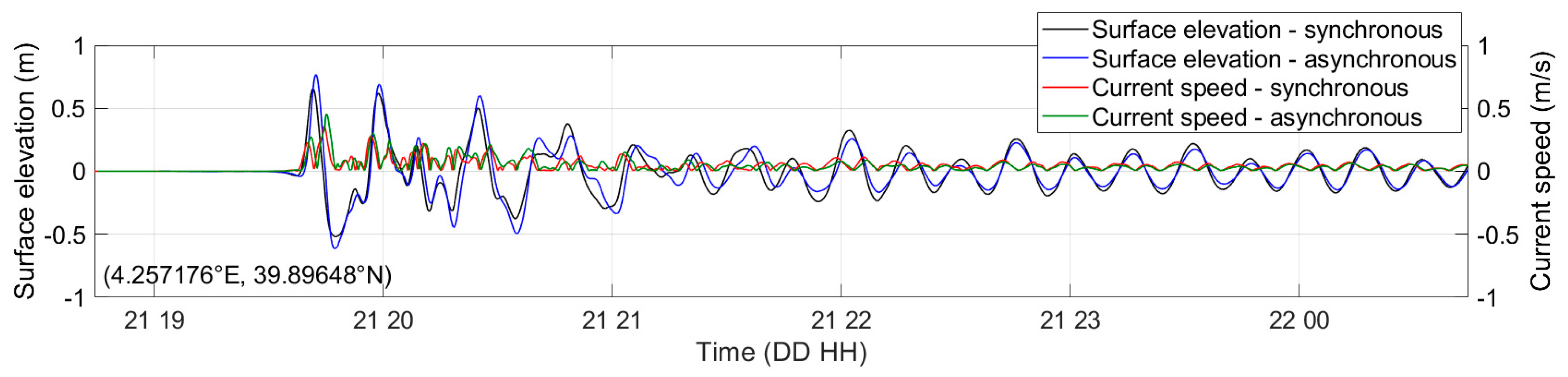
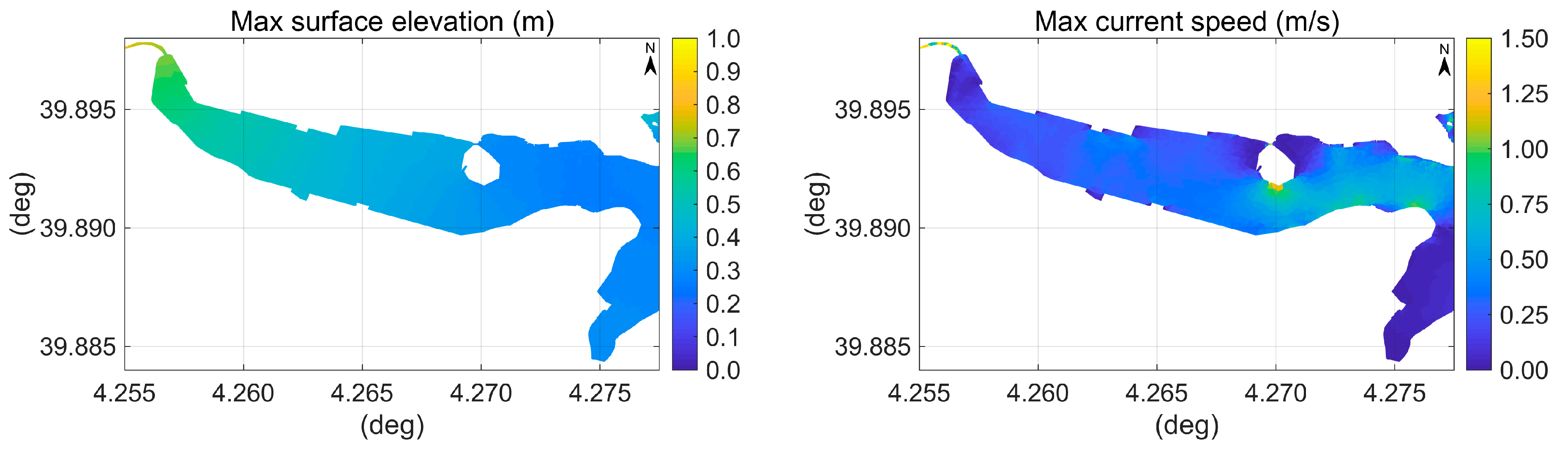
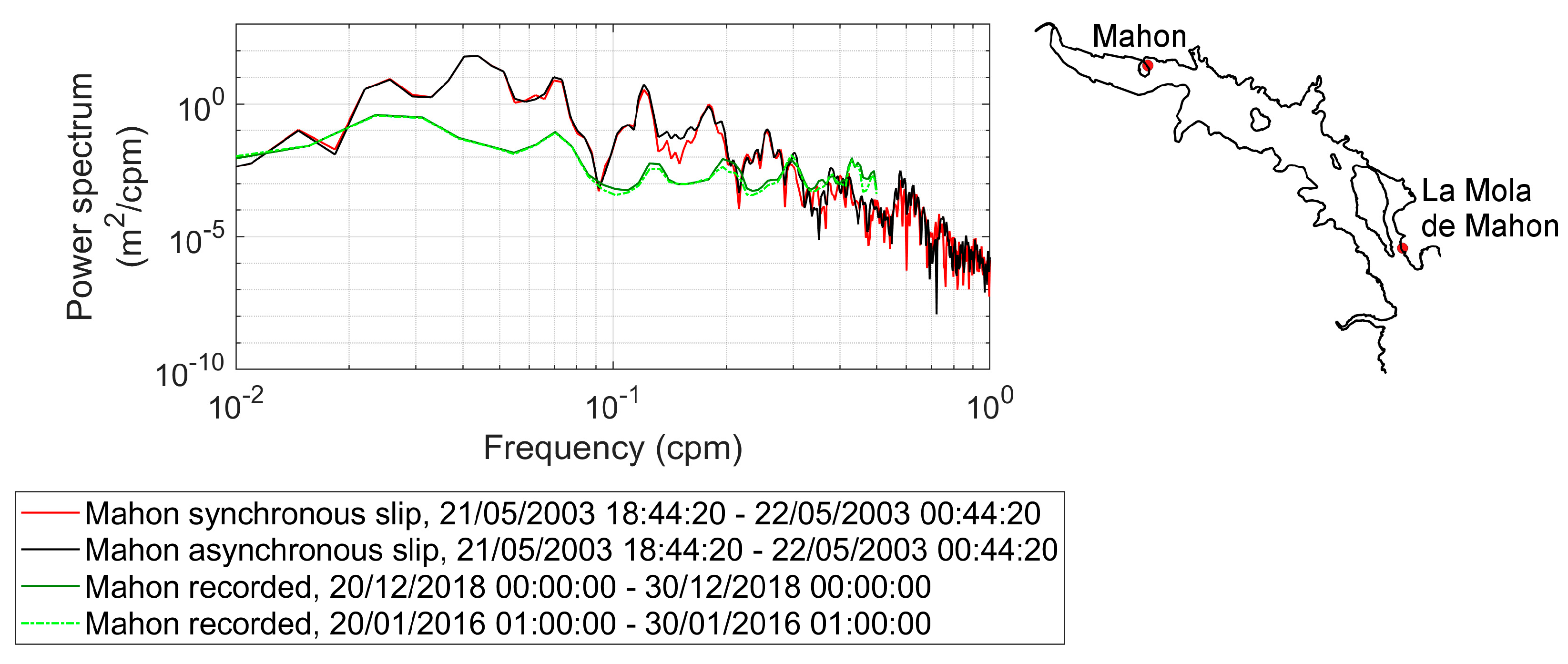
Figure 19 shows the spatial distribution of the maximum water surface elevations reached at the coasts of Eivissa and Formentera Islands during the 6 h tsunami simulation.
The highest water surface elevation on the entire computational domain, 1.26 m, is obtained at the end of the Sant Antoni de Portmany bay along the stretch of sandy beach in front of Avenida Doctor Fleming, as shown in detail in the upper plot of Figure 20. This elevated tsunami surge may be held responsible both for the flooding at the Sant Antoni coasts indicated by press reports and for damage to pier decks. Water levels higher than 1 m are found throughout the innermost part of the Sant Antoni bay from the port breakwater to the corresponding location on the southern side. The maximum water drawdown observed on the entire domain is −1.43 m, which is reached in the extreme northeast corner of the Sant Antoni port.
The maximum tsunami-induced current speeds estimated inside the Sant Antoni bay over the 6 h tsunami simulation are presented in the bottom plot of Figure 20. The highest current speeds, around 3.5 m/s, occur at the head of the port breakwater. Current speeds of ~1.7 m/s are found at Punta de Pinet, while slightly lower intensities are observed at Punta des Molí (~1.4 m/s) and in front of the shipyard in the central harbor area (~1.2 m/s).
The comparison between the power spectra of the background and tsunami oscillations recorded at the Sant Antoni tide gauge is shown in Figure 21. It highlights an energetic spectral peak at 21 min, which is absent in the background spectrum, therefore related to the properties of the tsunami forcing and common to all the investigated stations, and a resonant period of 16.7 min corresponding to the fundamental (Helmholtz) mode of the innermost part of the bay, from the shoreline down to 20 m water depth, corresponding to the nodal line (high velocity and low level oscillation) between Punta Xinxó and Punta de ses Variades. From Figure 22 it may be seen that the 21 min period is present from the tsunami arrival until 3:00 of the following day, during which waves reach the port following different paths. The existence of these two close spectral peaks generates beats which are clear in Figure 3 and Figure 22. In Figure 12 it is also evident the positive interference near the port of waves passing west and east of Eivissa Island. The rapid growth of oscillation mode amplitude demonstrates the strong interaction between the oscillation mode and the tsunami wave associated to the similar direction of induced currents. The combination of positive interference and strong resonance explains the highest level observed in Sant Antoni among other Balearic ports.
Regarding the port of Ibiza, maximum water surface elevations of about 0.6 m over the 6 h simulation are reached in all the innermost areas, while the maximum drawdown varies from −0.52 m in the most sheltered northern marina down to −0.60 m at the end of Marina Botafoch. The maximum current speed, ~2.2 m/s, is reached at the head of the breakwater protecting the port on the western side. Furthermore, current speeds of ~1.6 m/s are found at the head of the Marina Botafoch breakwater and ~1 m/s in the sheltered entrance. Flow intensities of ~1.5 m/s are also reached in the shallow waters at the end of the adjacent Cala Talamanca edged by a sandy beach.
However, in all these locations characterized by current speeds ≥1 m/s there are no moored boats and therefore the modeling results are substantially in agreement with irrelevant damages reported by press. The low oscillation amplitude reached in the port is the result of refraction on the continental platform, that concentrates energy in adjacent zones, see Figure 12 and Figure 19, and lack of resonance; in fact the analysis of recent tidal records (1 min time resolution) in good weather conditions has pointed out resonant periods around 40, 14, and 7 min. Lastly, from Figure 19 it is possible to observe that also the harbor of Santa Eulària des Riu is particularly exposed to the incoming tsunami waves. High water surface elevations and large drawdown affect the innermost zone of the harbor, while strong currents are generated at the entrance, capable of causing damage to boats and docks according to observations in press reports. Due to the shallow water depth of the Ensenada de Santa Eulària, the entire bay is prone to tsunami impact.

5.4. Port of Mahon

The spatial distribution of the maximum water surface elevations obtained in Port Mahon over the 6 h tsunami simulation from the asynchronous slip distribution pattern is presented in Figure 23 with enlargements in the left plots of Figure 24 and Figure 25.
Within the calculation domain, the highest water levels occur in four different zones: at Punta Prima (0.71 m), at the western end of Cala de Sant Esteve (0.86 m), at Cala Teulera (0.69 m), and at the inner end of the Mahon port (0.79 m). At Punta Prima local tsunami amplification occurs because of the shoaling effect at the open sea sandy beach.
The computed maximum water surface drawdown reaches −1.37 m at the end of Cala de Sant Esteve, just south of Port Mahon, while in the shallow north edge of Cala Teulera with water depth less than 5 m, it varies approximately from −0.90 down to −1.0 m at the entrance of the artificial channel Canal de Sant Jordi. A maximum drawdown value of −0.64 m is found in the innermost harbor zone of Mahon.
As shown in the right plot of Figure 24, tsunami-induced currents reach a significant intensity past the entrance of the port as a result of the shallower water depths in this area. Current speeds exceeding 1.5 m/s are found a little further ahead the entrance of Port Mahon, in correspondence of the abrupt water depth reduction from −12 m to −6 m entering the cove Cala Teulera, between Illa del Llatzeret and the peninsula of La Mola, and along the shallow water Canal de Sant Jordi. However, no damage was reported in this part of the port, also because anchoring in Cala Teulera is officially forbidden (only permitted when all other marinas are full or in case of bad weather conditions [127]). Strong currents exceeding 1.5 m/s are also obtained from numerical simulation in the narrow Cala de Sant Esteve with rocky seafloor (Figure 24). In addition to the effects caused by the sudden sea level variation, damage also due to tsunami-induced currents must be taken into consideration in this area, confirming the observed noticeable impact.
Current speed intensifies between Punta de Cala Figuera (~1 m/s), where berthing facilities are concentrated, and the opposite shore, as shown in the right plot of Figure 25. It is also noted that vessels moored in the area beginning from Punta de Cala Figuera and extending westward along the Levante Quay, where the Mediterranean style of berthing is used, were certainly exposed to the impact of significant transverse currents.
Computed time histories of water surface elevation and current speed at a virtual station at depth ~2.4 m located at the Colàrsega, in the inner end of Port Mahon, where severe damages were reported, are shown in Figure 26. The numerical results highlight a maximum surface elevation of 0.66 and 0.77 m using the synchronous and asynchronous slip distribution respectively and modest tsunami-induced current speeds. The spatial pattern for the synchronous slip distribution in the inner part of Port Mahon is shown in Figure 27; the patterns are similar with the greater intensity in the case of the asynchronous slip.
An area characterized by very small water level variations is evident in Figure 23, roughly extending between Illa del Rei and Illa del Llatzeret.
Unfortunately, no gauge station was in operation at tsunami time inside Port Mahon. However, two tide gauges have recently been installed: the first became operational by Puertos del Estado in October 2009 at Illa d’en Pinto (Figure 28), while the other, which has been activated in October 2017 on the north side of the entrance to the port at La Mola de Mahon, is part of the Sea Level Network of Inexpensive Device for Sea Level Measurement deployed by the Joint Research Centre of the European Commission with the specific objective to improve the monitoring of tsunami events in the Mediterranean Sea. The 1 min data collected by these two stations are freely accessible from the Sea Level Station Monitoring Facility website (http://www.ioc-sealevelmonitoring.org/) and have been used to estimate the effect of the local topobathymetric characteristics of the monitoring sites during calm weather periods. Figure 28 shows the power spectra for the selected background periods at Illa d’en Pinto (solid and dash-dotted lines in dark and light green). The main peak in the background power spectra is related to the fundamental Helmholtz mode of the harbor with period of about 42.7 min. Two other peaks at 14.2 and 8 min are evident which are associated with the following longitudinal modes of the port, being periods equal respectively to 1/3 and 1/5 of 42.7 min, in accordance with the formulation for the natural oscillation periods of a semi-enclosed rectangular basin with constant depth, e.g., [128]. Two additional high frequency peaks at 3.4 and 5.1 min may be identified in the Mahon spectra linked to the articulated harbor shape. No resonant period is evident from the background spectrum of La Mola. Further comparison between the background spectra and the tsunami spectra obtained from the simulated time series at the Mahon tide gauge location considering both synchronous and asynchronous slip reveals that the energy content of the external forcing is concentrated at about 23 min. Moreover, since the tsunami period lies between the fundamental and the second natural periods of the harbor, it seems that there was no particular resonance amplification of the event.
From the analysis of the tsunami simulation results, Cala Llonga does not seem to be affected neither by strong sea level oscillation nor by currents of particular intensity, as instead the damage reported for this location would suggest. Photographs of the bay end available at the website http://www.disfrutalaplaya.com/en/Menorca/Mao/Playa-Cala-Llonga.html (pictures 1 and 6) show the really shallow water depth of the area, a fixed pier with deck of limited height and the Mediterranean berthing style, all characters exposing boats to a higher tsunami hazard. Based only on the information given by press reports, the modeling results might seem to underestimate the tsunami impact, in addition to Cala Llonga, also in the innermost harbor zone, near the Colàrsega and Port d’Hivernada, but it is necessary to highlight that no additional detail is given on the type and size of the sunken and damaged boats, their draft and mooring conditions, their position before the tsunami, and no description of the type or cause of suffered damage is provided from which to infer the solicitation level applied by the tsunami. On the other hand, the port is naturally very well protected and might induce limited attention to mooring. The asynchronous sliding, according to our simulations, cannot explain a relevant increase of local agitation, being evaluated around +17% its effect at Mahon inner end (see Figure 26) and approximately +25% at Cala Llonga.

5.5. Damage Mechanisms and Thresholds

In these ports small to medium boats are normally present and often sailing boats with a deep keel, all of them having different scale and shape when compared to large ships. Therefore different damaging scenarios have to be considered. They fall into three categories:
  • mooring breakage and ship moved around hitting other ships or structures by (1) strong currents, (2) large water level oscillation with short and tight mooring;
  • ship lowered or raised by water level (1) hitting the bottom with keel or rudder, (2) raised and transported over the wharf, (3) raised against a fixed pier or a bridge and then sunk by still rising sea level;
  • ship caught in a breaker capsizes and sinks.
Some of the described damage mechanisms to vessels in ports can be found visualized in videos or photographs publicly available on the web (Table 5).
Lynett et al. [9] and the research team operating in California, based mainly on the experience coming from 2010 Maule (Chile) and 2011 Tohoku (Japan) tsunamis that arrived both in California at low tide conditions, have fixed the very simple threshold system: damages are not relevant if current intensity does not exceed 3 knots, damage is moderate if current does not exceed 6 knots, major if it does not exceed 9 knots, and extreme beyond this intensity. The threshold results not evidently dependent on vessel size.
However, besides current intensity, an extreme level is also a hazard factor for boats or small ships. Several observed damages to boats require also the introduction of a wave amplitude threshold as introduced by Suppasri et al. [123]. In fact, current speed drops to zero at bay end, whereas in these areas level oscillation reaches its maximum and most damages were observed. Let η c and η t be the maximum crest elevation a.m.s.l. and trough depth b.m.s.l. respectively, h the water depth at berth, D the ship draft, F’ the height where the ship can safely lean against the quay-wall, F the ship freeboard, W the wharf elevation, W’ the lower deck elevation and γb the breaker index, the following conditions need to be satisfied for a proper ship mooring at a fixed wharf
η t   <   m i n   ( h     D ,   F     W )   and   η c   <   m i n   ( W     F ,   γ b · h )
in order, respectively, not to hit the seabed, not to be caught under the deck, and not to be thrown on wharf, not to be caught in a breaker (and capsized). In the case of a floating berth only the first and last conditions are significant. A sketch illustrating the parameters considered for a boat and a fixed wharf is presented in Figure 29. However, for a boat, for which all the mentioned ship/wharf dimensions are small compared to the ship case, these conditions become more severe than the current speed condition. The above mentioned level amplitude conditions can explain damages occurred to boats in harbor sites where current was not exceeding any of the proposed thresholds.
The loss function developed by the Japanese research team, Muhari et al. [124], allows to evaluate the loss (percentage of the equipment value) based on tsunami parameters, i.e., height and speed, and non-exceedance probability, see Table 4 in [124]. The effect of displacement is not pointed out because the data set is dominated by small marine vessels weighting less than 5 tons. It shows for instance that complete loss (Loss > 90%) for half of the cases/boats (Probability = 0.50) is associated to tsunami height = 1.90 m or current speed = 2.10 m/s. The same tsunami parameters cause significant loss (Loss > 25%) to 3 out of 4 cases/boats.
As already observed in [124] the Japanese and Californian speed thresholds are consistent if “moderate” is considered equivalent to “1/2 of the involved vessels suffered a severe damage” and “major” to “3/4 of the involved vessels suffered a severe damage”. The tsunami height threshold is new; tsunami height threshold, whose values are reliable only for small vessels, and current speed threshold are highly correlated (Figure 30), whereas tsunami loading parameters in specific harbor conditions are independent, so that usually only one of them results critical for damaging.
In order to compare the damage probability of the criterion with actual damage frequency, the number of boats present in harbor at tsunami arrival time has been tentatively estimated by considering the present berth capacity and its evolution since 2003, as well as the annual cycle of presence different in permanent or seasonal ports. The estimated number is presented in Table 6 with the assessed tsunami parameters and a synthesis of damages. Damaging can be classified between minor and moderate depending on the harbor (Figure 30); the severity perception of the event is highlighted by its mention in port information: only for Port Mahon the event is quoted as a shelter failure causing substantial damages to yachts.
Globally these damage frequency data are fairly consistent with Muhari et al. [124] criterion, in particular if one realizes that important solicitation parameters, as the boat-current angle for instance, as well as the mooring resistance, are not explicitly considered. Mooring resistance is probably proportioned to sea waves, so that the best sheltered harbor, Port Mahon, results the most exposed to tsunami damage.
Considering all the boats damaged by the tsunami of 21 May 2003 in relation to the current number of berths in Balearic Islands, it is reasonable to hypothesize a percentage of damage around a few percentage points. It is therefore necessary to consider the stress induced inside the Balearic Islands ports by the described tsunami loading factors having a recurrence time of about 40 years, not considering tsunamis of meteorological origin. This information can also help to develop and implement appropriate tsunami hazard mitigation strategies for the individual harbors.

6. Conclusions

The Boumerdès earthquake of 21 May 2003 generated a tsunami that was recorded by tide gauges throughout the Western Mediterranean and caused severe damage to vessels and nautical facilities in the Balearic Islands ports. The proper wave period was about 21 min, but oscillation in harbor may have slightly different periods due to resonance selective amplification.
Slip distribution patterns and earthquake fault geometries, derived by studies of literature focused on the determination of the source rupture process, result in significant variation of the simulated tsunami and therefore in the predicted impact on exposed coastal areas.
Numerical tsunami simulation based on the slip distribution pattern derived from the planar fault model proposed by Belabbès et al. [34] with a motivated higher moment magnitude, Mw ~ 7.2 instead of the official 6.8–6.9, presents in general better agreement with the tsunami observations at Palma de Mallorca and Sant Antoni tide gauges, as well as at distant coasts, due to the higher simulated sea surface elevations and larger drawdown.
An evident delay in the range 4.4–6.0 min is found in our reconstruction at Palma de Mallorca tide gauge between observed and hindcasted tsunami arrival times, but it is also present in all previous studies even if using different simulation models. Additional investigation is required on this time shift, as it is not constant among ports and observed oscillations are characterized by more irregular behavior than those deriving from the simulations with the adopted modeling, especially in the initial stage.
A space-time dynamic displacement of the seabed might be more suitable than an instantaneous rupture for modeling the tsunami generation, as the trend of the radiated seismic energy shown in Figure 1 and Figure 12 seems to suggest. The space-time structure of the source displacement may change the radiation direction and tsunami intensity in the different ports.
The spectral analysis performed on the detided records of the tsunami event at Palma and Sant Antoni shows a dominant peak at periods of 21–23 min which is associated with the tsunami source characteristics and is well reproduced by the numerical models at all harbor sites. Some of the harbor natural oscillation modes, identified in the corresponding background spectra, were excited at the tsunami arrival. In particular, local tsunami wave amplification was favored at Palma de Mallorca and Sant Antoni, due to resonance effects of the bay-port system. Resonance, through a selective amplification of components, causes a shift of tsunami periods toward the bay resonance periods.
Excellent agreement is found inside the ports of Palma de Mallorca and Sant Antoni between critical areas derived from simulation and the tsunami affected zones indicated by newspapers, online news, or previous research studies.
A detailed tsunami simulation has been performed also for Port Mahon, where major damages to vessels and docks are documented, and the modeled hydrodynamic features have been correlated with the available, albeit qualitative, damage information from press reports.
By comparison with press information, the modeled tsunami impact associated to a synchronous sliding appears to be underestimated at the inner end of Port Mahon and particularly in Cala Llonga. Underestimation of tsunami effects inside the port of Mahon might be caused by a slightly inaccurate strike orientation of the fault plane and/or by asynchronous sliding, both causing several degrees deviation of the radiation lobe and consequent alteration of wave amplitude in the different ports.
The numerical dispersion of MIKE 21 Flexible Mesh, through lateral spreading and/or longitudinal dissipation, might be a cause of underestimation of hindcasted extremes, even if this underestimation is common to simulations of most tsunami events.
Numerical modeling provided tsunami solicitation parameters that can locally cause damage to vessels. The current speed thresholds proposed by Lynett et al. [9] are confirmed in a broad sense also by the present analysis. The threshold limits for tsunami height proposed by Suppasri et al. [123] and Muhari et al. [124] are broadly consistent with observations. Unfortunately, this threshold depends substantially on ship size and shape. Since both criteria do not represent explicitly the effects of the boat-current angle on loading and of mooring resistance, the probability associated in [124] refers to the usual statistics of these variables and not to the specific conditions.
The modeling procedure based on shallow water equations and results presented here may be used to assess tsunami hazard conditions, at least within Mediterranean harbors and ports, identifying areas where mooring is less safe under tsunami attack. The use of Boussinesq approximation, representing wave dispersion, might produce better results at the expense of greater computing load; it is suggested for a second approximation.

Author Contributions

M.M. proposed the study, manually digitized coastline and bathymetric data, ran the numerical simulations, analyzed tide gauge data and simulation results, wrote the original draft and the revised version of the manuscript. R.A. commented on the manuscript and provided funding for publication. A.L. supervised the study and the manuscript. All authors have read and agreed to the published version of the manuscript.

Funding

This research was partially funded by the University of Bologna that supported Marinella Masina in her research activity.

Acknowledgments

The authors wish to thank Carlo Zumaglini (Siap+Micros s.r.l.) and ISPRA for having provided the measurements collected by the Italian tide gauge network; Marta Marcos (IMEDEA) for making available the Sant Antoni tidal records and Pilar Gil Blázquez (Puertos del Estado) for the provision of the Malaga and Valencia tide gauge data. The authors would like to extend warm thanks to Joaquin Tintoré and Lluis Gómez-Pujol for the provision of the Balearic Islands bathymetric data owned by SOCIB and Miguel Tuduri of the Autoritat Portuaria de Balears for having provided the bathymetric map of the Palma de Mallorca harbor. We gratefully acknowledge all the organizations mentioned in the paper that made their data freely accessible online. We are grateful to Guillem Xavier Pons Buades and Vicent Marí for providing the permission to include the photographs in Figure 13 documenting damages to boats. Thanks are extended to Andrea Pedroncini (DHI-Italia) for his technical support.

Conflicts of Interest

The authors declare no conflict of interest.

References

  1. Dilley, M.; Chen, R.S.; Deichmann, U.; Lerner-Lam, A.L.; Arnold, M.; Agwe, J.; Buys, P.; Kjekstad, O.; Lyon, B.; Yetman, G. Natural Disaster Hotspots: A Global Risk Analysis. Disaster Risk Management Series No. 5-34423; The World Bank: Washington, DC, USA, 2005. [Google Scholar]
  2. International Tsunami Information Center. Available online: http://itic.ioc-unesco.org/index.php (accessed on 22 July 2020).
  3. NOAA National Centers for Environmental Information. National Geophysical Data Center/World Data Service: NCEI/WDS Global Historical Tsunami Database. Available online: https://www.ngdc.noaa.gov/hazard/tsu_db.shtml (accessed on 24 July 2020).
  4. Maramai, A.; Brizuela, B.; Graziani, L. The Euro-Mediterranean Tsunami Catalogue. Ann. Geophys. 2014, 57, S0435. [Google Scholar] [CrossRef]
  5. Goeldner-Gianella, L.; Grancher, D.; Robertsen, Ø.; Anselme, B.; Brunstein, D.; Lavigne, F. Perception of the risk of tsunami in a context of high-level risk assessment and management: The case of the fjord Lyngen in Norway. Geoenviron. Disasters 2017, 4, 227. [Google Scholar] [CrossRef] [Green Version]
  6. Cerase, A.; Crescimbene, M.; La Longa, F.; Amato, A. Tsunami risk perception in southern Italy: First evidence from a sample survey. Nat. Hazards Earth Syst. Sci. 2019, 19, 2887–2904. [Google Scholar] [CrossRef] [Green Version]
  7. Giles, J.; Marris, E. Indonesian tsunami-monitoring system lacked basic equipment. Nature 2004. [Google Scholar] [CrossRef]
  8. Melgar, D.; Bock, Y. Near-field tsunami models with rapid earthquake source inversions from land- and ocean-based observations: The potential for forecast and warning. J. Geophys. Res. Solid Earth 2013, 118, 5939–5955. [Google Scholar] [CrossRef]
  9. Lynett, P.J.; Borrero, J.; Son, S.; Wilson, R.; Miller, K. Assessment of the tsunami-induced current hazard. Geophys. Res. Lett. 2014, 41, 2048–2055. [Google Scholar] [CrossRef]
  10. Yelles-Chaouche, A.K.; Djellit, H.; Hamdache, M. The Boumerdes -Algiers (Algeria) Earthquake of May 21st, 2003 (Mw = 6.8). In CSEM/EMSC Newsletter N; 20 September 2003; pp. 3–5. Available online: https://www.emsc-csem.org/Files/docs/data/newsletters/newsletter_20.pdf (accessed on 26 July 2020).
  11. Laouami, N.; Slimani, A.; Bouhadad, Y.; Nour, A.; Larbes, S. Analysis of Strong Ground Motions Recorded during the 21st May, 2003 Boumerdes, Algeria, Earthquake. In CSEM/EMSC Newsletter N; 20 September 2003; pp. 5–7. Available online: https://www.emsc-csem.org/Files/docs/data/newsletters/newsletter_20.pdf (accessed on 26 July 2020).
  12. Laouami, N.; Slimani, A.; Bouhadad, Y.; Chatelain, J.-L.; Nour, A. Evidence for fault-related directionality and localized site effects from strong motion recordings of the 2003 Boumerdes (Algeria) earthquake: Consequences on damage distribution and the Algerian seismic code. Soil Dyn. Earthq. Eng. 2006, 26, 991–1003. [Google Scholar] [CrossRef]
  13. EERI, Earthquake Engineering Research Institute. The Boumerdes, Algeria, Earthquake of May 21, 2003. EERI Learning from Earthquakes, Reconnaissance Report; EERI Publication Number 2003-04; EERI: Oakland, CA, USA, 2003; Available online: https://www.eeri.org/site/images/lfe/pdf/algeria_20030521.pdf (accessed on 27 July 2020).
  14. Meghraoui, M.; Maouche, S.; Chemaa, B.; Cakir, Z.; Aoudia, A.; Harbi, A.; Alasset, P.-J.; Ayadi, A.; Bouhadad, Y.; Benhamouda, F. Coastal uplift and thrust faulting associated with the Mw = 6.8 Zemmouri (Algeria) earthquake of 21 May, 2003. Geophys. Res. Lett. 2004, 31, L19605. [Google Scholar] [CrossRef] [Green Version]
  15. Papadopoulos, G.A.; Gràcia, E.; Urgeles, R.; Sallares, V.; De Martini, P.M.; Pantosti, D.; González, M.; Yalciner, A.C.; Mascle, J.; Sakellariou, D.; et al. Historical and pre-historical tsunamis in the Mediterranean and its connected seas: Geological signatures, generation mechanisms and coastal impacts. Mar. Geol. 2014, 354, 81–109. [Google Scholar] [CrossRef]
  16. Peláez, J.A.; Chourak, M.; Tadili, B.A.; Aït Brahim, L.; Hamdache, M.; López Casado, C.; Martínez Solares, J.M. A catalog of main Moroccan earthquakes from 1045 to 2005. Seism. Res. Lett. 2007, 78, 614–621. [Google Scholar] [CrossRef]
  17. Hamdache, M.; Peláez, J.A.; Talbi, A.; López Casado, C. A unified catalog of main earthquakes for Northern Algeria from A.D. 856 to 2008. Seism. Res. Lett. 2010, 81, 732–739. [Google Scholar] [CrossRef] [Green Version]
  18. Soloviev, S.L.; Solovieva, O.N.; Go, C.N.; Kim, K.S.; Shchetnikov, N.A. Tsunamis in the Mediterranean Sea 2000 B.C.-2000 A.D. In Advances in Natural and Technological Hazards Research, Volume 13; Kluwer Academic Publishers: Dordrecht, The Netherlands, 2000. [Google Scholar]
  19. Roger, J.; Hébert, H. The 1856 Djijelli (Algeria) earthquake and tsunami: Source parameters and implications for tsunami hazard in the Balearic Islands. Nat. Hazards Earth Syst. Sci. 2008, 8, 721–731. [Google Scholar] [CrossRef] [Green Version]
  20. Harbi, A.; Meghraoui, M.; Maouche, S. The Djidjelli (Algeria) earthquakes of 21 and 22 August 1856 (I0 VIII, IX) and related tsunami effects Revisited. J. Seism. 2011, 15, 105–129. [Google Scholar] [CrossRef]
  21. Maouche, S.; Harbi, A.; Meghraoui, M. Attenuation of intensity for the Zemmouri earthquake of 21 May 2003 (Mw 6.8): Insights for the seismic hazard and historical earthquake sources in Northern Algeria. In Historical Seismology. Interdisciplinary Studies of Past and Recent Earthquakes. Modern Approaches in Solid Earth Sciences; Fréchet, J., Meghraoui, M., Stucchi, M., Eds.; Springer: Dordrecht, The Netherlands, 2008; Volume 2, pp. 327–350. [Google Scholar] [CrossRef]
  22. Bezzeghoud, M.; Dimitro, D.; Ruegg, J.C.; Lammali, K. Faulting mechanism of the El Asnam (Algeria) 1954 and 1980 earthquakes from modelling of vertical movements. Tectonophysics 1995, 249, 249–266. [Google Scholar] [CrossRef]
  23. Hébert, H.; Alasset, P.-J. The tsunami triggered by the 21 May 2003 Algiers earthquake. In CSEM/EMSC Newsletter N.; 20 September 2003; pp. 10–12. Available online: https://www.emsc-csem.org/Files/docs/data/newsletters/newsletter_20.pdf (accessed on 26 July 2020).
  24. Wang, X.; Liu, P.L.-F. A numerical investigation of Boumerdes-Zemmouri (Algeria) earthquake and tsunami. Comput. Model. Eng. Sci. 2005, 10, 171–184. [Google Scholar] [CrossRef]
  25. Borrero, J.C. Preliminary Simulations of the Algerian Tsunami of 21 May, 2003 in the Balearic Islands; University of Southern California: Los Angeles, CA, USA, 2003. [Google Scholar]
  26. Alasset, P.-J.; Hébert, H.; Maouche, S.; Calbini, V.; Meghraoui, M. The tsunami induced by the 2003 Zemmouri earthquake (MW = 6.9, Algeria): Modelling and results. Geophys. J. Int. 2006, 166, 213–226. [Google Scholar] [CrossRef] [Green Version]
  27. Delouis, B.; Vallée, M.; Meghraoui, M.; Calais, E.; Maouche, S.; Lammali, K.; Mahsas, A.; Briole, P.; Benhamouda, F.; Yelles, K. Slip distribution of the 2003 Boumerdes-Zemmouri earthquake, Algeria, from teleseismic, GPS, and coastal uplift data. Geophys. Res. Lett. 2004, 31, L18607. [Google Scholar] [CrossRef] [Green Version]
  28. Yelles, K.; Lammali, K.; Mahsas, A.; Calais, E.; Briole, P. Coseismic deformation of the May 21st, 2003, Mw = 6.8 Boumerdes earthquake, Algeria, from GPS measurements. Geophys. Res. Lett. 2004, 31, L13610. [Google Scholar] [CrossRef]
  29. Semmane, F.; Campillo, M.; Cotton, F. Fault location and source process of the Boumerdes, Algeria, earthquake inferred from geodetic and strong motion data. Geophys. Res. Lett. 2005, 32, L01305. [Google Scholar] [CrossRef] [Green Version]
  30. Sahal, A.; Roger, J.; Allgeyer, S.; Lemaire, B.; Hébert, H.; Schindelé, F.; Lavigne, F. The tsunami triggered by the 21 May 2003 Boumerdès-Zemmouri (Algeria) earthquake: Field investigations on the French Mediterranean coast and tsunami modelling. Nat. Hazards Earth Syst. Sci. 2009, 9, 1823–1834. [Google Scholar] [CrossRef]
  31. Vela, J.; Pérez, B.; González, M.; Otero, L.; Olabarrieta, M.; Canals, M.; Casamor, J.L. Tsunami resonance in the Palma de Majorca bay and harbour induced by the 2003 Boumerdes-Zemmouri Algerian earthquake (Western Mediterranean). In Proceedings of the 32nd International Conference on Coastal Engineering 2010, Shanghai, China, 30 June–5 July 2010; McKee Smith, J., Lynett, P., Eds.; ASCE/COPRI Coastal Engineering Research Council: Reston, VA, USA, 2011. currents.7. [Google Scholar] [CrossRef] [Green Version]
  32. Vela, J.; Pérez, B.; González, M.; Otero, L.; Olabarrieta, M.; Canals, M.; Casamor, J.L. Tsunami resonance in Palma bay and harbor, Majorca Island, as induced by the 2003 Western Mediterranean earthquake. J. Geol. 2014, 122, 165–182. [Google Scholar] [CrossRef] [Green Version]
  33. Samaras, A.G.; Karambas, T.V.; Archetti, R. Simulation of tsunami generation, propagation and coastal inundation in the Eastern Mediterranean. Ocean Sci. 2015, 11, 643–655. [Google Scholar] [CrossRef] [Green Version]
  34. Belabbès, S.; Wicks, C.; Çakir, Z.; Meghraoui, M. Rupture parameters of the 2003 Zemmouri (Mw 6.8), Algeria, earthquake from joint inversion of interferometric synthetic aperture radar, coastal uplift, and GPS. J. Geophys. Res. Solid Earth 2009, 114, B03406. [Google Scholar] [CrossRef]
  35. Nocquet, J.-M.; Calais, E. Geodetic measurements of crustal deformation in the Western Mediterranean and Europe. Pure Appl. Geophys. 2004, 161, 661–681. [Google Scholar] [CrossRef]
  36. Serpelloni, E.; Vannucci, G.; Pondrelli, S.; Argnani, A.; Casula, G.; Anzidei, M.; Baldi, P.; Gasperini, P. Kinematics of the Western Africa-Eurasia plate boundary from focal mechanisms and GPS data. Geophys. J. Int. 2007, 169, 1180–1200. [Google Scholar] [CrossRef]
  37. Bounif, A.; Dorbath, C.; Ayadi, A.; Meghraoui, M.; Beldjoudi, H.; Laouami, N.; Frogneux, M.; Slimani, A.; Alasset, P.J.; Kharroubi, A.; et al. The 21 May 2003 Zemmouri (Algeria) earthquake Mw 6.8: Relocation and aftershock sequence analysis. Geophys. Res. Lett. 2004, 31, L19606. [Google Scholar] [CrossRef]
  38. Bourenane, H.; Bouhadad, Y.; Tas, M. Liquefaction hazard mapping in the city of Boumerdès, Northern Algeria. Bull. Eng. Geol. Environ. 2018, 77, 1473–1489. [Google Scholar] [CrossRef] [Green Version]
  39. Yagi, Y. Preliminary Results of Rupture Process. Available online: http://iisee.kenken.go.jp/staff/yagi/eq/algeria20030521/algeria2003521.html (accessed on 3 December 2016).
  40. Yagi, Y. Source process of large and significant earthquakes in 2003. Bull. Int. Inst. Seismol. Earthq. Eng. 2003, 37, 145–153. [Google Scholar]
  41. Delouis, B.; Vallée, M. The 2003 Boumerdes (Algeria) earthquake: Source process from teleseismic data. In CSEM/EMSC Newsletter N; 20 September 2003; pp. 8–9. Available online: https://www.emsc-csem.org/Files/docs/data/newsletters/newsletter_20.pdf (accessed on 26 July 2020).
  42. Bezzeghoud, M.; Caldeira, B.; Borges, J.F.; Beldjoudi, H.; Buforn, E.; Maouche, S.; Ousadou, F.; Kherroubi, A.; Harbi, A.; Ayadi, A. The Zemmouri-Boumerdes (Algeria) Earthquake of May 21st, 2003, Mw=6.8: Source Parameters and Rupture Propagation Study from Teleseismic Data; European Seismological Commission—XXIX General Assembly, University & GFZ: Potsdam, Germany, 2004. [Google Scholar]
  43. Braunmiller, J.; Bernardi, F. The 2003 Boumerdes, Algeria earthquake: Regional moment tensor analysis. Geophys. Res. Lett. 2005, 32, L06305. [Google Scholar] [CrossRef] [Green Version]
  44. Santos, R.; Caldeira, B.; Bezzeghoud, M.; Borges, J.F. The rupture process and location of the 2003 Zemmouri-Boumerdes earthquake (Mw 6.8) inferred from seismic and geodetic data. Pure Appl. Geophys. 2015, 172, 2421–2434. [Google Scholar] [CrossRef] [Green Version]
  45. Bossu, R.; Godey, S.; Mazet-Roux, G. EMSC actions concerning the Boumerdes-Zemmouri event. In CSEM/EMSC Newsletter N; 20 September 2003; p. 2. Available online: https://www.emsc-csem.org/Files/docs/data/newsletters/newsletter_20.pdf (accessed on 26 July 2020).
  46. Bernardi, F. Earthquake Source Parameters in the Alpine-Mediterranean Region from Surface Wave Analysis. Ph.D. Thesis, ETH Nr. 15652. Swiss Federal Institute of Technology, Zürich, Switzerland, 2004. [Google Scholar] [CrossRef]
  47. Déverchère, J.; Yelles, K.; Domzig, A.; Mercier de Lépinay, B.; Bouillin, J.-P.; Gaullier, V.; Bracène, R.; Calais, E.; Savoye, B.; Kherroubi, A.; et al. Active thrust faulting offshore Boumerdes, Algeria, and its relations to the 2003 Mw 6.9 earthquake. Geophys. Res. Lett. 2005, 32, L04311. [Google Scholar] [CrossRef] [Green Version]
  48. Déverchère, J.; Mercier de Lépinay, B.; Cattaneo, A.; Strzerzynski, P.; Calais, E.; Domzig, A.; Bracene, R. Comment on “Zemmouri earthquake rupture zone (Mw 6.8, Algeria): Aftershocks sequence relocation and 3D velocity model” by A. Ayadi et al. J. Geophys. Res. Solid Earth 2010, 115, B04320. [Google Scholar] [CrossRef] [Green Version]
  49. Kherroubi, A.; Yelles-Chaouche, A.; Koulakov, I.; Déverchère, J.; Beldjoudi, H.; Haned, A.; Semmane, F.; Aidi, C. Full aftershock sequence of the Mw 6.9 2003 Boumerdes earthquake, Algeria: Space-time distribution, local tomography and seismotectonic implications. Pure Appl. Geophys. 2017, 174, 2495–2521. [Google Scholar] [CrossRef]
  50. IRIS DMC. Data Services Products: EQEnergy Earthquake Energy & Rupture Duration; IRIS: Washington, DC, USA, 2013. [Google Scholar] [CrossRef]
  51. Convers, J.A.; Newman, A.V. Global evaluation of large earthquake energy from 1997 through mid-2010. J. Geophys. Res. Solid Earth 2011, 116, B08304. [Google Scholar] [CrossRef] [Green Version]
  52. Heezen, B.C.; Ewing, M. Orléansville earthquake and turbidity currents. AAPG Bull. 1955, 39, 2505–2514. [Google Scholar] [CrossRef]
  53. El-Robrini, M.; Gennesseaux, M.; Mauffret, A. Consequences of the El-Asnam earthquakes: Turbidity currents and slumps on the Algerian margin (Western Mediterranean). Geo-Mar. Lett. 1985, 5, 171–176. [Google Scholar] [CrossRef]
  54. Cattaneo, A.; Babonneau, N.; Ratzov, G.; Dan-Unterseh, G.; Yelles, K.; Bracène, R.; Mercier de Lépinay, B.; Boudiaf, A.; Déverchère, J. Searching for the seafloor signature of the 21 May 2003 Boumerdès earthquake offshore central Algeria. Nat. Hazards Earth Syst. Sci. 2012, 12, 2159–2172. [Google Scholar] [CrossRef] [Green Version]
  55. Bryant, E. Tsunami: The Underrated Hazard, 2nd ed.; Springer, Praxis Publishing Ltd.: Chichester, UK, 2008. [Google Scholar]
  56. Harbi, A.; Maouche, S.; Ousadou, F.; Rouchiche, Y.; Yelles-Chaouche, A.; Merahi, M.; Heddar, A.; Nouar, O.; Kherroubi, A.; Beldjoudi, H.; et al. Macroseismic Study of the Zemmouri Earthquake of 21 May 2003 (Mw 6.8, Algeria). Earthq. Spectra 2007, 23, 315–332. [Google Scholar] [CrossRef]
  57. Edwards, C.L. Zemmouri, Algeria, Mw 6.8 Earthquake of May 21, 2003. In Technical Council on Lifeline Earthquake Engineering, Monograph No. 27; Edwards, C.L., Ed.; The American Society of Civil Engineers: Reston, VA, USA, 2004. [Google Scholar]
  58. Vich, M.-d.-M.; Monserrat, S. Source spectrum for the Algerian tsunami of 21 May 2003 estimated from coastal tide gauge data. Geophys. Res. Lett. 2009, 36, L20610. [Google Scholar] [CrossRef] [Green Version]
  59. Heidarzadeh, M.; Satake, K. The 21 May 2003 tsunami in the Western Mediterranean Sea: Statistical and wavelet analyses. Pure Appl. Geophys. 2013, 170, 1449–1462. [Google Scholar] [CrossRef]
  60. Toda, S.; Stein, R.S.; Sevilgen, V.; Lin, J. Coulomb 3.3 Graphic-Rich Deformation and Stress-Change Software for Earthquake, Tectonic, and Volcano Research and Teaching-User Guide; US Geological Survey Open-File Report 2011-1060; 2011. Available online: https://pubs.usgs.gov/of/2011/1060/ (accessed on 29 July 2020).
  61. Okada, Y. Internal deformation due to shear and tensile faults in a half-space. Bull. Seismol. Soc. Am. 1992, 82, 1018–1040. [Google Scholar]
  62. Nosov, M.A.; Bolshakova, A.V.; Kolesov, S.V. Displaced water volume, potential energy of initial elevation, and tsunami intensity: Analysis of recent tsunami events. Pure Appl. Geophys. 2014, 171, 3515–3525. [Google Scholar] [CrossRef]
  63. Levin, B.W.; Nosov, M.A. Physics of Tsunamis, 2nd ed; Springer International Publishing: Cham, Switzerland, 2016. [Google Scholar] [CrossRef]
  64. Kajiura, K. The leading wave of a tsunami. Bull. Earthq. Res. Ins. Univ. Tokyo 1963, 41, 535–571. [Google Scholar]
  65. Saito, T.; Furumura, T. Three-dimensional tsunami generation simulation due to sea-bottom deformation and its interpretation based on the linear theory. Geophys. J. Int. 2009, 178, 877–888. [Google Scholar] [CrossRef]
  66. Lynett, P.J.; Borrero, J.C.; Weiss, R.; Son, S.; Greer, D.; Renteria, W. Observations and modeling of tsunami-induced currents in ports and harbors. Earth Planet. Sci. Lett. 2012, 327–328, 68–74. [Google Scholar] [CrossRef]
  67. Lynett, P.J.; Gately, K.; Wilson, R.; Montoya, L.; Arcas, D.; Aytore, B.; Bai, Y.; Bricker, J.D.; Castro, M.J.; Cheung, K.F.; et al. Inter-model analysis of tsunami-induced coastal currents. Ocean Model. 2017, 114, 14–32. [Google Scholar] [CrossRef]
  68. Arcos, M.E.M.; LeVeque, R.J. Validating velocities in the GeoClaw tsunami model using observations near Hawaii from the 2011 Tohoku tsunami. Pure Appl. Geophys. 2015, 172, 849–867. [Google Scholar] [CrossRef] [Green Version]
  69. Barberopoulou, A.; Legg, M.R.; Uslu, B.; Synolakis, C.E. Reassessing the tsunami risk in major ports and harbors of California I: San Diego. Nat. Hazards 2011, 58, 479–496. [Google Scholar] [CrossRef]
  70. Bolaños, R.; Sørensen, J.V.T.; Benetazzo, A.; Carniel, S.; Sclavo, M. Modelling ocean currents in the northern Adriatic Sea. Cont. Shelf Res. 2014, 87, 54–72. [Google Scholar] [CrossRef]
  71. Haigh, I.D.; Wijeratne, E.M.S.; MacPherson, L.R.; Pattiaratchi, C.B.; Mason, M.S.; Crompton, R.P.; George, S. Estimating present day extreme water level exceedance probabilities around the coastline of Australia: Tides, extra-tropical storm surges and mean sea level. Clim. Dyn. 2014, 42, 121–138. [Google Scholar] [CrossRef]
  72. Masina, M.; Archetti, R.; Besio, G.; Lamberti, A. Tsunami taxonomy and detection from recent Mediterranean tide gauge data. Coast. Eng. 2017, 127, 145–169. [Google Scholar] [CrossRef]
  73. Sarker, M.A. Numerical modelling of tsunami in the Makran Subduction Zone-A case study on the 1945 event. J. Oper. Oceanogr. 2019, 12, S212–S229. [Google Scholar] [CrossRef]
  74. Leschka, S.; Kongko, W.; Larsen, O. On the influence of nearshore bathymetry data quality on tsunami runup modelling, part II: Modelling. In Proceedings of the 5th International Conference on Asian and Pacific Coasts 2009; Tan, S.K., Huang, Z., Eds.; World Scientific Pub Co Pte Ltd.: Singapore, 2009; pp. 157–163. [Google Scholar] [CrossRef]
  75. Gayer, G.; Leschka, S.; Nöhren, I.; Larsen, O.; Günther, H. Tsunami inundation modelling based on detailed roughness maps of densely populated areas. Nat. Hazards Earth Syst. Sci. 2010, 10, 1679–1687. [Google Scholar] [CrossRef] [Green Version]
  76. Kaiser, G.; Scheele, L.; Kortenhaus, A.; Løvholt, F.; Römer, H.; Leschka, S. The influence of land cover roughness on the results of high resolution tsunami inundation modeling. Nat. Hazards Earth Syst. Sci. 2011, 11, 2521–2540. [Google Scholar] [CrossRef] [Green Version]
  77. Payande, A.R.; Niksokhan, M.H.; Naserian, H. Tsunami hazard assessment of Chabahar bay related to megathrust seismogenic potential of the Makran subduction zone. Nat. Hazards 2015, 76, 161–176. [Google Scholar] [CrossRef]
  78. Boswood, P.K. Tsunami Modelling along the East Queensland Coast, Report 1: Regional Modelling; Department of Science, Information Technology, Innovation and the Arts, Queensland Government: Brisbane, Queensland, Australia, 2013. Available online: https://publications.qld.gov.au/dataset/tsunami-modelling-east-queensland-coast (accessed on 26 July 2020).
  79. Barua, D.K.; Allyn, N.F.; Quick, M.C. Modeling tsunami and resonance response of Alberni Inlet, British Columbia. In Proceedings of the 30th International Conference on Coastal Engineering 2006, San Diego, CA, USA, 3–8 September 2006; McKee Smith, J., Ed.; World Scientific Pub Co Pte Ltd.: Singapore, 2007; pp. 1590–1602. [Google Scholar] [CrossRef] [Green Version]
  80. Zhang, Y.; Onodera, M.; Carr, C. Modelling of resonance response of Dawei Seaport to tsunami waves. In Proceedings of the 34th International Conference on Coastal Engineering 2014, Seoul, Korea, 15–20 June 2014; Lynett, P., Ed.; ASCE/COPRI Coastal Engineering Research Council: Reston, VA, USA, 2014. currents.29. [Google Scholar] [CrossRef] [Green Version]
  81. Winckler, P.; Sepúlveda, I.; Aron, F.; Contreras-López, M. How do tides and tsunamis interact in a highly energetic channel? The case of Canal Chacao, Chile. J. Geophys. Res. Oceans 2017, 122, 9605–9624. [Google Scholar] [CrossRef] [Green Version]
  82. DHI. MIKE 21 Flow Model FM, Hydrodynamic Module, User Guide; Danish Hydraulic Institute: Hørsholm, Denmark, 2011. [Google Scholar]
  83. Tintoré, J.; Vizoso, G.; Casas, B.; Heslop, E.; Pascual, A.; Orfila, A.; Ruiz, S.; Martínez-Ledesma, M.; Torner, M.; Cusí, S.; et al. SOCIB: The Balearic Islands Coastal Ocean Observing and Forecasting System responding to science, technology and society needs. Mar. Technol. Soc. J. 2013, 47, 101–117. [Google Scholar] [CrossRef]
  84. Pagine Azzurre. Il Portolano dei Mari d’Italia, 2014 ed.; Pagine Azzurre s.r.l.: Rome, Italy, 2014. [Google Scholar]
  85. Smagorinsky, J. General circulation experiments with the primitive equations: I. The basic experiment. Mon. Weather Rev. 1963, 91, 99–164. [Google Scholar] [CrossRef]
  86. Kowalik, Z. Introduction to Numerical Modeling of Tsunami Waves; Institute of Marine Science, University of Alaska: Fairbanks, AK, USA, 2012; Available online: https://uaf.edu/cfos/files/research-projects/people/kowalik/book_sum.pdf (accessed on 28 July 2020).
  87. Flather, R.A. A tidal model of the northwest European continental shelf. Mem. Soc. R. Sci. Liège 1976, 6, 141–164. [Google Scholar]
  88. Palma, E.D.; Matano, R.P. On the implementation of passive open boundary conditions for a general circulation model: The barotropic mode. J. Geophys. Res. Oceans 1998, 103, 1319–1341. [Google Scholar] [CrossRef]
  89. Marchesiello, P.; McWilliams, J.C.; Shchepetkin, A. Open boundary conditions for long-term integration of regional oceanic models. Ocean Model. 2001, 3, 1–20. [Google Scholar] [CrossRef]
  90. Roe, P.L. Approximate Riemann solvers, parameter vectors, and difference schemes. J. Comput. Phys. 1981, 43, 357–372. [Google Scholar] [CrossRef]
  91. DHI. MIKE 21 & MIKE 3 Flow Model FM—Hydrodynamic and Transport Module. Scientific Documentation; Danish Hydraulic Institute: Hørsholm, Denmark, 2017. [Google Scholar]
  92. Jawahar, P.; Kamath, H. A high-resolution procedure for Euler and Navier-Stokes computations on unstructured grids. J. Comput. Phys. 2000, 164, 165–203. [Google Scholar] [CrossRef]
  93. Hirsch, C. Numerical Computation of Internal and External Flows, Volume 2: Computational Methods for Inviscid and Viscous Flows; Wiley: Chichester, UK, 1990. [Google Scholar]
  94. Darwish, M.S.; Moukalled, F. TVD schemes for unstructured grids. Int. J. Heat Mass Transf. 2003, 46, 599–611. [Google Scholar] [CrossRef]
  95. Díaz del Río, V. El ‘tsunami’ que llegó de Argelia. El País. 25 June 2003. Available online: https://elpais.com/diario/2003/06/25/futuro/1056492007_850215.html (accessed on 16 February 2020).
  96. Tel, E.; González, M.-J.; Ruiz, C.; García, M.-J. Sea level data archaeology: Tsunamis and Seiches and other phenomena. In Proceedings of the 4a Assembleia Luso Espanhola de Geodesia e Geofísica, Figueira da Foz, Portugal, 3–7 February 2004. [Google Scholar]
  97. Basterretxea, G.; Orfila, A.; Jordi, A.; Casas, B.; Lynett, P.; Liu, P.L.F.; Duarte, C.M.; Tintoré, J. Seasonal dynamics of a microtidal pocket beach with posidonia oceanica seabeds (Mallorca, Spain). J. Coast. Res. 2004, 20, 1155–1164. [Google Scholar] [CrossRef] [Green Version]
  98. Gailler, A.; Hébert, H.; Schindelé, F.; Reymond, D. Coastal amplification laws for the French Tsunami Warning Center: Numerical modeling and fast estimate of tsunami wave heights along the French Riviera. Pure Appl. Geophys. 2018, 175, 1429–1444. [Google Scholar] [CrossRef]
  99. Luger, S.A.; Harris, R.L. Modelling tsunamis generated by earthquakes and submarine slumps using Mike 21. In Proceedings of the International MIKE by DHI Conference ‘Modelling in a World of Change’, Copenhagen, Denmark, 6–8 September 2010; p. 17. [Google Scholar]
  100. ABC (Madrid). 23 May 2003, p. 27. Available online: https://www.abc.es/archivo/periodicos/abc-madrid-20030523-27.html (accessed on 3 September 2020).
  101. Bureau de Recherches Géologiques et Minières (BRGM). Base de données des tsunamis observés en France. Available online: http://tsunamis.brgm.fr/fiche_biblio.asp?NUMEVT=60004 (accessed on 31 December 2016).
  102. www.belt.es. 26 May 2003. Available online: http://www.belt.es/noticias/2003/mayo/26/baleares.htm (accessed on 31 December 2016).
  103. La Vanguardia. 23 May 2003, p. 37. Available online: http://hemeroteca-paginas.lavanguardia.com/LVE01/PUB/2003/05/23/LVG200305230371LB.pdf (accessed on 3 September 2020).
  104. Roig-Munar, F.X.; Martín-Prieto, J.Á.; Rodríguez-Perea, A.; Gelabert Ferrer, B.; Vilaplana Fernández, J.M. Bloques en plataformas rocosas y acantilados del SE de Menorca: Tipología y procesos. In Geomorfología Litoral de Menorca: Dinámica, evolución y prácticas de gestión, Monografies de la Societat d’Història Natural de les Balears; Gómez-Pujol, L., Pons, G.X., Eds.; Societat d’Història Natural de les Balears: Palma, Illes Balears, 2017; Volume 25, pp. 251–262. [Google Scholar]
  105. Libertad Digital. 22 May 2003. Available online: http://www.libertaddigital.com/sociedad/numerosas-embarcaciones-y-puertos-de-baleares-han-sufrido-danos-a-causa-del-terremoto-1275760565/ (accessed on 3 September 2020).
  106. Papadopoulos, G.A. Tsunamis in the European-Mediterranean Region: From Historical Record to Risk Mitigation; Elsevier: Amsterdam, The Netherlands, 2016. [Google Scholar]
  107. Consell d’Eivissa. Plan territorial insular de protección civil de la isla de Eivissa -Platerei- Documento de Consulta. Available online: http://www.conselldeivissa.es/portal/RecursosWeb/DOCUMENTOS/1/0_5186_1.pdf (accessed on 3 September 2020).
  108. Periódico de Ibiza y Formentera. 24 May 2003. Available online: https://www.periodicodeibiza.es/sucesos/ultimas/2003/05/24/722787/las-pitiuses-fueron-las-%20islas-que-menos-sufrieron-el-maremoto.html (accessed on 3 September 2020).
  109. Diario de Ibiza. 26 August 2011. Available online: http://www.diariodeibiza.es/pitiuses-balears/2011/08/26/sistema-alerta-maremotos-mediterraneoafronta-primer-gran-ensayo/503113.html (accessed on 3 September 2020).
  110. Azurseisme. Site sur la sismicité historique régionale. Available online: https://www.azurseisme.com/Tsunami-english-version.html (accessed on 3 September 2020).
  111. Periódico de Ibiza y Formentera, 28 October 2010. Available online: https://www.periodicodeibiza.es/pitiusas/ibiza/2010/10/28/24008/el-peligro-que-llega-del-mar.html (accessed on 3 September 2020).
  112. El Mundo, 22 May 2003. Available online: https://www.elmundo.es/elmundo/2003/05/22/sociedad/1053590416.html (accessed on 3 September 2020).
  113. Fritz, H.M.; Phillips, D.A.; Okayasu, A.; Shimozono, T.; Liu, H.; Mohammed, F.; Skanavis, V.; Synolakis, C.E.; Takahashi, T. The 2011 Japan tsunami current velocity measurements from survivor videos at Kesennuma Bay using LiDAR. Geophys. Res. Lett. 2012, 39, L00G23. [Google Scholar] [CrossRef]
  114. Okal, E.A.; Fritz, H.M.; Raad, P.E.; Synolakis, C.; Al-Shijbi, Y.; Al-Saifi, M. Oman field survey after the December 2004 Indian Ocean tsunami. Earthq. Spectra 2006, 22, 203–218. [Google Scholar] [CrossRef]
  115. Okal, E.A.; Fritz, H.M.; Raveloson, R.; Joelson, G.; Pančošková, P.; Rambolamanana, G. Madagascar field survey after the December 2004 Indian Ocean tsunami. Earthq. Spectra 2006, 22, 263–283. [Google Scholar] [CrossRef]
  116. Okal, E.A.; Sladen, A.; Okal, E.A.-S. Rodrigues, Mauritius, and Réunion Islands field survey after the December 2004 Indian Ocean tsunami. Earthq. Spectra 2006, 22, 241–261. [Google Scholar] [CrossRef]
  117. Wilson, R.I.; Admire, A.R.; Borrero, J.C.; Dengler, L.A.; Legg, M.R.; Lynett, P.; McCrink, T.P.; Miller, K.M.; Ritchie, A.; Sterling, K.; et al. Observations and impacts from the 2010 Chilean and 2011 Japanese tsunamis in California (USA). Pure Appl. Geophys. 2013, 170, 1127–1147. [Google Scholar] [CrossRef]
  118. Admire, A.R.; Dengler, L.A.; Crawford, G.B.; Uslu, B.U.; Borrero, J.C.; Greer, S.D.; Wilson, R.I. Observed and modeled currents from the Tohoku-oki, Japan and other recent tsunamis in Northern California. Pure Appl. Geophys. 2014, 171, 3385–3403. [Google Scholar] [CrossRef]
  119. Borrero, J.C.; Lynett, P.J.; Kalligeris, N. Tsunami currents in ports. Phil. Trans. R. Soc. A 2015, 373, 20140372. [Google Scholar] [CrossRef] [PubMed] [Green Version]
  120. Lynett, P.; Weiss, R.; Renteria, W.; De La Torre Morales, G.; Son, S.; Arcos, M.E.M.; MacInnes, B.T. Coastal impacts of the March 11th Tohoku, Japan tsunami in the Galapagos Islands. Pure Appl. Geophys. 2013, 170, 1189–1206. [Google Scholar] [CrossRef] [Green Version]
  121. Borrero, J.C.; Bell, R.; Csato, C.; DeLange, W.; Goring, D.; Greer, S.D.; Pickett, V.; Power, W. Observations, effects and real time assessment of the March 11, 2011 Tohoku-oki tsunami in New Zealand. Pure Appl. Geophys. 2013, 170, 1229–1248. [Google Scholar] [CrossRef]
  122. Wilson, R.I.; Miller, K.M. Tsunami Emergency Response Playbooks and FASTER Tsunami Height Calculation: Background Information and Guidance for Use. California Geological Survey Special Report 236; California Department of Conservation, California Geological Survey: Sacramento, CA, USA, 2014. [Google Scholar]
  123. Suppasri, A.; Muhari, A.; Futami, T.; Imamura, F.; Shuto, N. Loss functions for small marine vessels based on survey data and numerical simulation of the 2011 Great East Japan tsunami. J. Waterw. Port Coast. Ocean Eng. 2014, 140, 04014018. [Google Scholar] [CrossRef]
  124. Muhari, A.; Charvet, I.; Tsuyoshi, F.; Suppasri, A.; Imamura, F. Assessment of tsunami hazards in ports and their impact on marine vessels derived from tsunami models and the observed damage data. Nat. Hazards 2015, 78, 1309–1328. [Google Scholar] [CrossRef] [Green Version]
  125. Rabinovich, A.B.; Thomson, R.E. The 26 December 2004 Sumatra tsunami: Analysis of tide gauge data from the World Ocean Part 1. Indian Ocean and South Africa. Pure Appl. Geophys. 2007, 164, 261–308. [Google Scholar] [CrossRef]
  126. Torrence, C.; Compo, G.P. A practical guide to wavelet analysis. Bull. Am. Meteor. Soc. 1998, 79, 61–78. [Google Scholar] [CrossRef] [Green Version]
  127. RCC Pilotage Foundation; Baggaley, D.; Baggaley, S. Islas Baleares: Ibiza, Formentera, Mallorca, Cabrera and Menorca, 11th ed.; Imray Laurie Norie & Wilson Ltd.: Cambridgeshire, UK, 2018. [Google Scholar]
  128. Rabinovich, A.B. Seiches and harbor oscillations. In Handbook of Coastal and Ocean Engineering; Kim, Y.C., Ed.; World Scientific Pub Co Pte Ltd.: Singapore, 2009; pp. 193–236. [Google Scholar]
Figure 1. Cumulative energy growth as a function of time for the 2003 Boumerdès earthquake; EQEnergy data from http://ds.iris.edu/ds/products/eqenergy, doi:10.17611/DP/1718531. Based on the procedure of Convers and Newman [51], the high frequency energy growth is used to identify the approximate event duration TR, while the total event energy is determined using broadband energy at TR.
Jmse 08 00933 g001
Figure 2. Bathymetry of the Western Mediterranean Sea from the EMODnet Bathymetry portal. The red dots mark the location of the tide gauges available in the area during the 21 May 2003 tsunami event. The locations of the Boumerdès village and Mahon port are also indicated on the map as yellow dots.
Jmse 08 00933 g002
Figure 3. Tsunami records at Balearic Islands ports. 1 min sea level data from the Palma de Mallorca tide gauge are available from the SeaDataNet website; 2 min sea level measurements in Sant Antoni were provided by Dr. M. Marcos (IMEDEA); 5 min data from Ibiza tide gauge are delivered by Puertos del Estado; the vertical red line denotes the time of the earthquake (https://cdi.seadatanet.org/search; http://www.puertos.es/en-us/oceanografia/Pages/portus.aspx).
Jmse 08 00933 g003
Figure 4. Tsunami records at Spanish ports. 5 min sea level data from Barcelona, Valencia and Malaga tide gauges are delivered by Puertos del Estado. 10 min measurements at Alicante 1, Alicante 2 and Almeria are provided by Instituto Geográfico Nacional (https://www.ign.es/web/ign/portal/gds-red-mareografos). The vertical red line denotes the time of the earthquake.
Jmse 08 00933 g004
Figure 5. Tsunami records at French ports. 10 min sea level measurements from Monaco-Fontvieille, Nice, Toulon, Marseille and Ajaccio-Aspretto tide gauges are delivered by SHOM (http://data.shom.fr/). 5 min sea level data from Senetosa M3 and M4 are available from AVISO+ website (https://www.aviso.altimetry.fr/data/calval/in-situ/absolute-calibration/download-tide-gauge-data.html). The vertical red line denotes the time of the earthquake.
Jmse 08 00933 g005
Figure 6. Tsunami records at Italian ports. Sea level measurements with 10 min sampling interval are delivered by Higher Institute for Environmental Protection and Research (ISPRA). The vertical red line denotes the time of the earthquake.
Jmse 08 00933 g006
Figure 7. Initial water surface elevation estimated for each considered source model of the 21 May 2003 Boumerdès earthquake: (a) Yelles et al. [28], (b) Delouis et al. [27], (c) Meghraoui et al. [14], (d) Semmane et al. [29], (e) Braunmiller and Bernardi [43], (f) modified from that estimated by Belabbès et al. [34], and (g) Santos et al. [44].
Jmse 08 00933 g007
Figure 8. Progressively refined computational mesh generated for the Sant Antoni bay.
Jmse 08 00933 g008
Figure 9. Comparison of tsunami waveforms simulated from different slip distributions and detided records at Palma de Mallorca and Cagliari.
Jmse 08 00933 g009
Figure 10. Comparison of tsunami waveforms computed using the slip distribution derived from that proposed by Belabbès et al. [34] with detided sea level records at Sant Antoni, Ibiza, and Valencia.
Jmse 08 00933 g010
Figure 11. Coseismic slip distribution of the 21 May 2003 Boumerdès earthquake modified from the source model proposed by Belabbès et al. [34].
Jmse 08 00933 g011
Figure 12. Crest elevation during tsunami propagation from Algeria to Balearic Islands: (a) synchronous movement along the fault plane, (b) 60 s delayed eastern sliding. Several effects are made evident: the main radiation direction, wave amplification due to shoaling at Balearic continental margin and, due also to refraction, at Menorca SE cape. The simulated delay of the eastern sliding causes a reorientation of the radiation lobe with a significant intensification at Menorca Island. The maximum surface elevation is increased east of the ray reaching Palma with accentuation on the edge of the Balearic continental shelf, while to the west of this ray it is reduced. The window in the upper left corner of figure (b) describes the difference (b-a) between the two solutions around Menorca Island where the maximum effect along the mentioned edge is observed. The figure was generated using the DHI MATLAB Toolbox.
Jmse 08 00933 g012
Figure 13. Photographs documenting damages to boats caused by the 21 May 2003 tsunami at the Balearic Islands. (a) A sunken boat in Sant Antoni, derived from [109]; reproduced with permission from Vicent Marí. (b) Boats accumulated at the end of the Cala de Sant Esteve, derived from [104]; reproduced with permission from Guillem Xavier Pons Buades. Other photographs are publicly accessible online at [103,111,112].
Jmse 08 00933 g013
Figure 14. Distribution of the maximum water surface elevations in the bay of Palma over the 6 h tsunami simulation. The undisturbed sea level used in the calculations is the LAT, the real one was 0.48 m above LAT.
Jmse 08 00933 g014
Figure 15. Distribution of the maximum water surface elevations (left plot) and maximum depth-averaged current speeds (right plot) in the port of Palma de Mallorca over the 6 h tsunami simulation. The black filled dot drawn in the left plot indicates the tide gauge location. Since the current pattern is less regular than that of the sea surface elevations, in order to provide an adequate visual representation the full scale of the colorbar is lower than the maximum value: in some points in the domain speed does actually exceed 2.5 m/s.
Jmse 08 00933 g015
Figure 16. Time histories of water surface elevation and current speed computed by the nested model at a virtual station (2.6340°E, 39.5680°N, 1.7 m depth below LAT) located inside the Palma de Mallorca port between the Sant Magí dock and the Royal Yatch Club, during the 21 May 2003 tsunami.
Jmse 08 00933 g016
Figure 17. Power spectra of the background (green line) and tsunami (black line) oscillations recorded at the Palma de Mallorca tide gauge. The power spectrum of the 6 h modeled time series, from 21 May 18:44:20 (earthquake time) to 22 May 00:44:20, at the tide gauge location inside the port is also shown (red line).
Jmse 08 00933 g017
Figure 18. Wavelet spectrum of the filtered Palma sea level data during the period from 21 May 15:00 to 23 May 00:00. The color scale shows the base 2 logarithm of wave energy.
Jmse 08 00933 g018
Figure 19. Spatial distribution of the maximum water surface elevations at Eivissa and Formentera Islands over the 6 h tsunami simulation from the asynchronous slip distribution pattern.
Jmse 08 00933 g019
Figure 20. Spatial distribution of the maximum water surface elevations and current speeds in the harbor of Sant Antoni de Portmany over the 6 h tsunami simulation from the asynchronous slip distribution pattern. The black filled dot drawn in the upper plot indicates the tide gauge location.
Jmse 08 00933 g020
Figure 21. Power spectra of the background (green line) and tsunami (black line) oscillations recorded at the Sant Antoni tide gauge.
Jmse 08 00933 g021
Figure 22. Wavelet spectrum of the filtered Sant Antoni sea level data during the period from 21 May 15:01 to 23 May 01:00. The color scale shows the logarithm of wave energy to the base 2.
Jmse 08 00933 g022
Figure 23. Spatial distribution of the maximum water surface elevations in SE Menorca over the 6 h tsunami simulation from the asynchronous slip distribution pattern.
Jmse 08 00933 g023
Figure 24. Spatial distribution of the maximum water surface elevations and current speeds in the eastern part of Port Mahon over the 6 h tsunami simulation from the asynchronous slip distribution pattern.
Jmse 08 00933 g024
Figure 25. Spatial distribution of the maximum water surface elevations and current speeds in the inner part of Port Mahon over the 6 h tsunami simulation from the asynchronous slip distribution pattern.
Jmse 08 00933 g025
Figure 26. Time histories of water surface elevation and current speed computed at a virtual station (2.4 m depth) in the inner end of Port Mahon, Colàrsega, considering the effect of both synchronous and asynchronous sliding on the tsunami generation.
Jmse 08 00933 g026
Figure 27. Spatial distribution of the maximum water surface elevations and current speeds in the inner part of Port Mahon over the 6 h tsunami simulation from the synchronous slip distribution pattern.
Jmse 08 00933 g027
Figure 28. Location of the Mahon and La Mola tide gauges (red dots) and comparison at Mahon between the power spectra of background sea level oscillations during calm weather periods and the power spectra of the modeled tsunami time series considering both the synchronous and asynchronous slip distribution.
Jmse 08 00933 g028
Figure 29. A sketch illustrating the parameters considered for a boat and a fixed wharf.
Jmse 08 00933 g029
Figure 30. Tsunami load parameters for small vessels and damage thresholds. Diamonds: Muhari et al. [124] threshold values. : less-than-full-damage domain and the corresponding probability. X-nn%: solicitation and frequency of vessel full damage in the analyzed harbor X (id in Table 6), estimated as the ratio of the number of totally damaged boats to the number of boats in the harbor.
Jmse 08 00933 g030
Table 1. Characteristics of the first arriving tsunami wave estimated from the Sant Antoni and Palma sea level records and results obtained from previous studies by numerical modeling.
SourceSea Level StationSimulated Fault MechanismMwArrival
Time
First Peak
Elevation
(m)
First Peak to
Trough
Height (m)
Sea level recordSant Antoni 19:450.370.99
Wang & Liu [24]Sant AntoniMeghraoui et al. [14]6.8–6.919:470.190.54
Wang & Liu [24]Sant AntoniWang & Liu [24]7.219:450.371.08
Alasset et al. [26]Sant AntoniMeghraoui et al. [14]6.8–6.919:470.070.19
Alasset et al. [26]Sant AntoniSemmane et al. [29]7.119:450.220.57
Sea level recordPalma 19:350.240.59
Alasset et al. [26]PalmaMeghraoui et al. [14]6.8–6.919:450.040.08
Alasset et al. [26]PalmaSemmane et al. [29]7.119:410.160.36
Vela et al. [31]PalmaMeghraoui et al. [14]6.8–6.919:410.090.24
Vela et al. [31]PalmaWang & Liu [24]7.219:410.120.30
Table 2. Estimated parameters of the 21 May 2003 Boumerdès earthquake.
SourceTime
(UTC)
Lon
(°E)
Lat
(°N)
Depth
(km)
M0
(N·m)
MwS/D/R
(°)
Fault Length
(km)
Fault Width
(km)
Data Type
CRAAG18:44:193.5836.9110 6.8
CGS18:44:403.5336.81 7.0
EMSC18:44:223.7637.0221 6.8
USGS NEIC18:44:193.7836.8910 6.7
USGS (2014)18:44:203.63436.964122.15 × 10196.855/30/90
Harvard CMT18:44:303.5836.93152.01 × 10196.857/44/71
CEA-DASE18:44:223.7836.7118 6.9
ETH 3.7437.0410 6.7463/35/48
INGV18:44:293.6136.90151.8 × 10196.865/27/86
Yagi [39,40] 3.7836.89102.4 × 10196.954/47/866010T
Delouis & Vallée [41] 102.38 × 10196.957/39/8350 T
Yelles et al. [28] 2.4 × 10196.955/42/843214G
Delouis et al. [27] 3.65 (B)36.83 (B)6.52.9 × 10196.970/45/956024T, G, U
Meghraoui et al. [14] 3.65 (B)36.83 (B) 2.75 × 10196.954/50/(90)54 U
Bezzeghoud et al. [42] 3.65 (B)36.83 (B)71.3 × 10196.864/50/90 T
Braunmiller & Bernardi [43]18:443.65 (B)36.83 (B) 7.062/25/8250 T
Semmane et al. [29] 3.65 (B)36.83 (B) 5.9 × 10197.154/47/886432G, U, M
Belabbès et al. [34], planar 3.65 (B)36.83 (B)81.78 × 10196.865/40/906030S, U, G
Belabbès et al. [34], curved 3.65 (B)36.83 (B)102.15 × 10196.865/40/90 S, U, G
Santos et al. [44], sol 1 3.66036.84681.40 × 10196.764/50/976020T, U, S
CRAAG—Center of Research in Astronomy, Astrophysics and Geophysics, Algeria, [10]; CGS—National Center of Applied Research in Earthquake Engineering, Algeria, [11,12]; EMSC—Euro-Mediterranean Seismological Center, https://www.emsc-csem.org/Doc/BOUMERDES_21052003/ALGER_long.txt, [45]; USGS NEIC—USGS National Earthquake Information Center, USA, http://www.indiana.edu/~pepp/earthquakes/images/algeria5_21_03/usgsmap.jpg. (accessed on 7 Jan 2017); USGS (2014)—United States Geological Survey, USA. Earthquake Catalog, last update of moment tensor in 2015, https://earthquake.usgs.gov/earthquakes/search/; Harvard CMT—Harvard Global Centroid Moment Tensor Catalog, http://www.globalcmt.org/CMTsearch.html; CEA-DASE—Commissariat à l’énergie atomique et aux énergies alternatives, Direction des applications militaires, Sciences de la Terre et de l’Environnement, France, http://www-dase.cea.fr/actu/dossiers_scientifiques/2003-05-21/index_en.html; ETH—Swiss Federal Institute of Technology, Switzerland, Table 4.1 in [46]; INGV—National Institute of Geophysics and Vulcanology, Italy, http://mednet.rm.ingv.it/procedure/events/QRCMT/030521_184422/qrcmt.gif. Longitude, latitude and depth of hypocenter. S/D/R are strike, dip and rake angles. M0 is the seismic moment and Mw the moment magnitude. Epicenter relocation from Bounif et al. [37] is indicated with (B). The last column indicates the type of data used to estimate the slip distribution: T = teleseismic data; U = coastal uplift measurements; G = GPS network data; M = strong motion data from accelerometric network stations; S = synthetic aperture radar data.
Table 3. Comparison between detided observations and simulated time series at the tide gauges by using different source models in terms of tsunami arrival time, maximum elevation and drawdown, rms sea level and mean zero-crossing period.
Tide
Gauge
Yelles
et al.
Delouis
et al.
Meghraoui
et al.
Semmane
et al.
Braunmiller
& Bernardi
Santos
et al.
Belabbès
et al.
Modified
Belabbès
et al.
Modified
Palma19:30–24:00Model globalglobalglobalglobalglobalglobalglobalnested
Arrival time19:3519:43:0419:42:5219:43:3419:41:3019:38:3619:42:5619:41:3619:41:38
Max elevation (m)0.640.170.140.100.270.080.100.410.43
Max drawdown (m)−0.52−0.17−0.14−0.09−0.27−0.09−0.11−0.43−0.45
RMS elevation (m)0.2510.0720.0570.0410.1140.0350.0440.1890.196
Mean period (min)22.722.422.422.322.522.722.422.522.5
Cagliari19:50–24:00Model nestednestednestednestednestednested nested
Arrival time20:0020:12:4220:10:5620:11:1220:08:3220:08:5020:14:06 20:11:24
Max elevation (m)0.160.050.060.030.120.060.03 0.20
Max drawdown (m)−0.16−0.05−0.04−0.02−0.10−0.05−0.03 −0.17
RMS elevation (m)0.0820.0220.0200.0130.0430.0220.013 0.070
Mean period (min)(33.3)28.128.428.128.628.528.0 28.4
Sant Antoni19:35–24:00Model nested
Arrival time19:45 19:44:14
Max elevation (m)1.11 1.10
Max drawdown (m)−0.85 −1.18
RMS elevation (m)0.314 0.306
Mean period (min)19.5 19.1
Ibiza19:25–24:00Model nested
Arrival time19:30 19:32:24
Max elevation (m)0.34 0.41
Max drawdown (m)−0.31 −0.36
RMS elevation (m)0.149 0.154
Mean period (min)22.1 16.4
Valencia19:55–24:00Model nested
Arrival time20:10 20:05:52
Max elevation (m)0.35 0.14
Max drawdown (m)−0.31 −0.13
RMS elevation (m)0.123 0.053
Mean period (min)20.0 20.5
Table 4. Simulation results using synchronous and asynchronous slip distribution along the fault plane in terms of zero-crossing time and extreme elevation at the tide gauge location in Palma de Mallorca and Sant Antoni and at a virtual station (4.257176°E, 39.89648°N) in Mahon port, compared with available observations.
Synchronous SlipAsynchronous SlipObservation
Zero-Crossing
Time (UTC)
Extreme
Elevation (m)
Zero-Crossing
Time (UTC)
Extreme
Elevation (m)
Zero-Crossing
Time (UTC)
Extreme
Elevation (m)
Palma de Mallorca19:41:36 19:42:06 19:35
0.145 0.147 0.24
19:54:28 19:54:54 19:49
−0.308 −0.301 −0.35
20:07:26 20:08:00 20:04
0.209 0.201 0.12
20:18:08 20:18:42 20:14
−0.184 −0.173 −0.13
20:26:38 20:27:12 20:22
Sant Antoni19:44:14 19:44:44 19:45
0.292 0.287 0.37
19:52:18 19:52:54 19:54
−0.589 −0.574 −0.62
20:02:34 20:03:04 20:04
1.101 1.089 1.11
20:11:24 20:11:52 20:12
−1.176 −1.160 −0.85
20:20:42 20:21:02 20:23
Mahon19:38:24 19:39:20
0.655 0.767
19:44:12 19:44:50
−0.521 −0.614
19:56:16 19:56:36
0.618 0.690
20:04:54 20:03:50
−0.114 −0.110
20:07:20 20:07:44
Table 5. Link to images representing tsunami damage mechanisms to vessels in ports from web sources.
Damage MechanismSourceImage
Boats touching the dry bottom of the harborhttps://www.youtube.com/watch?v=AxFNXRTXgHw
Santa Cruz Harbor, California, USA, 11 March 2011 tsunami
around 1:40/16:48
Boats captured in a tsunami borehttps://www.youtube.com/watch?v=jltIeWB1XH8
Santa Cruz Harbor, California, USA, 11 March 2011 tsunami
around 1:17/5:50
Boat wedged under a floating dockhttps://www.youtube.com/watch?v=AxFNXRTXgHw
Santa Cruz Harbor, California, USA, 11 March 2011 tsunami
around 8:52/16:48
Stranded shipshttp://www.cargolaw.com/2011nightmare_sendai_ships.html
Sendai, Japan, 11 March 2011 tsunami
several examples
Table 6. Extreme water surface elevation, drawdown, current speed and a summary of damage for the 21 May 2003 tsunami. Tsunami load parameters are evaluated as the greater between those referring to synchronous and asynchronous slip patterns. For current speed a typical value in the berth area is presented with the nodal maximum value in parentheses.
IdPort, BayPeak Surface Elevation
(m)
Peak Drawdown (m)Current Speed (m/s)Estimated n. of Boats in HarborReported Damage
APalma de Mallorca-Between Sant Magí dock and Royal Yacht Club up to La Riera+1.15−1.071.95 (2.1)1500Flooding, several boats damaged by grounding and collision
BSant Antoni-Near the fishermen pier+1.16−1.331.2 (1.4)150Flooding, 15 boats, port facilities
CPort Mahon-Colàrsega+0.79−0.640.7 (1.6)120Flooding, 37 boats, port facilities
DPort Mahon-Cala Llonga+0.51−0.470.6 (1.0)4520 boats, port facilities
ECala de Sant Esteve+0.86−1.372.2 (3.0)20Flooding, at least 5 boats stranded
Publisher’s Note: MDPI stays neutral with regard to jurisdictional claims in published maps and institutional affiliations.

