Continuous Coastal Monitoring with an Automated Terrestrial Lidar Scanner


Abstract
:1. Introduction
2. Methods: Data Collection and Processing
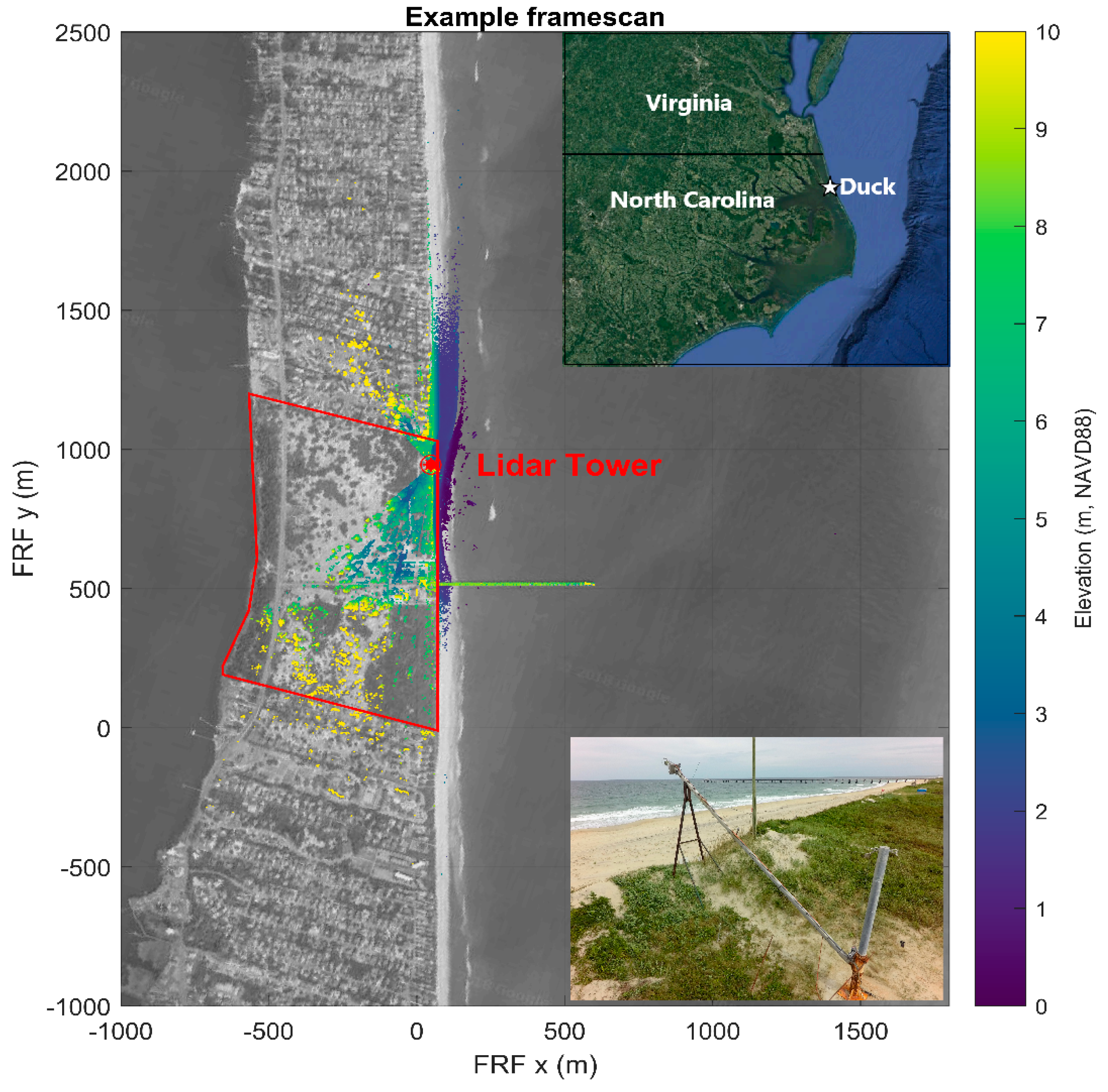
2.1. Field Site
2.2. Scanner Setup and Scan Collection
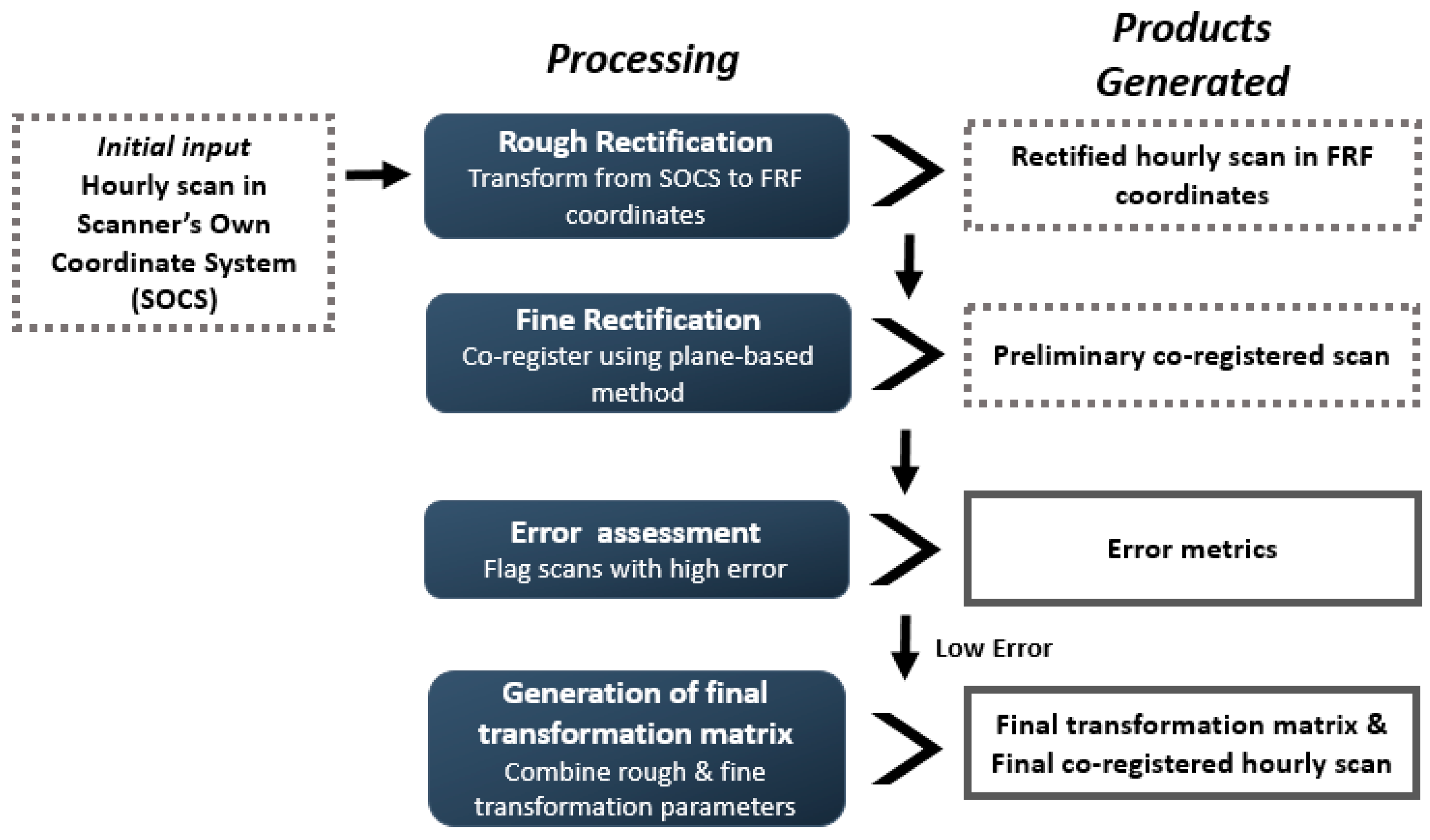
2.3. Processing Methods
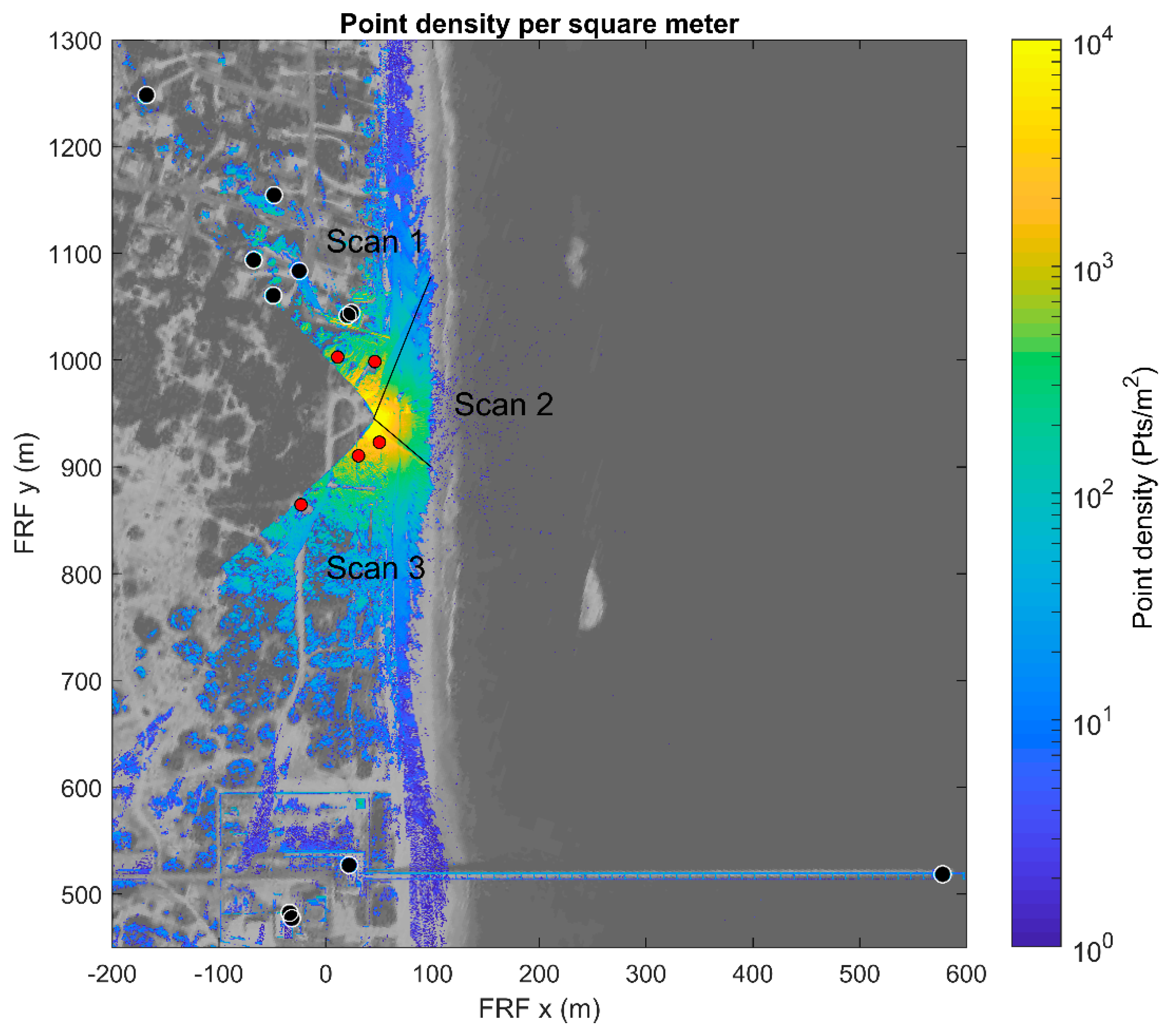
2.3.1. Geo-Referencing and Scan Alignment
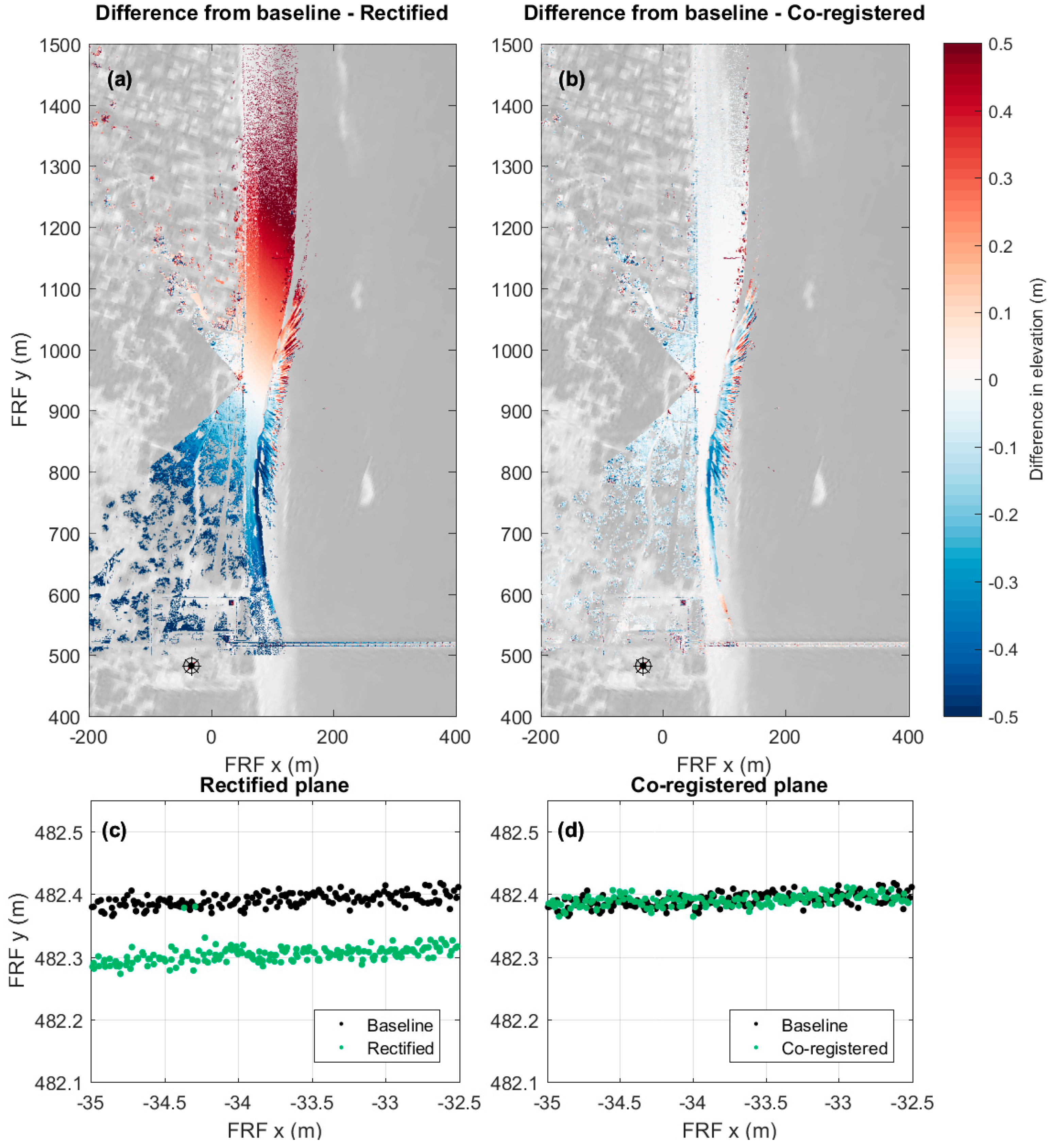
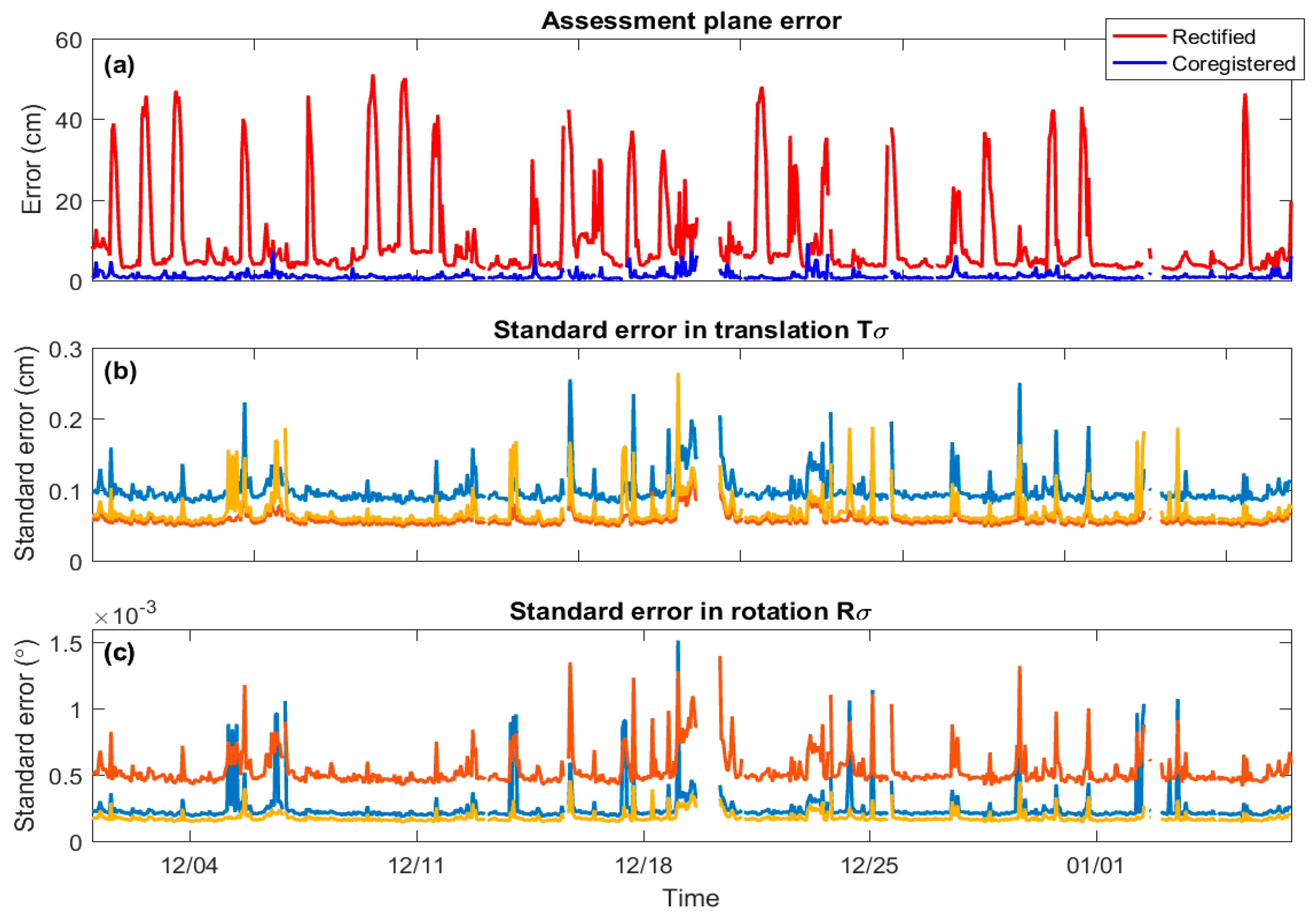
2.3.2. Co-registration Error Assessment
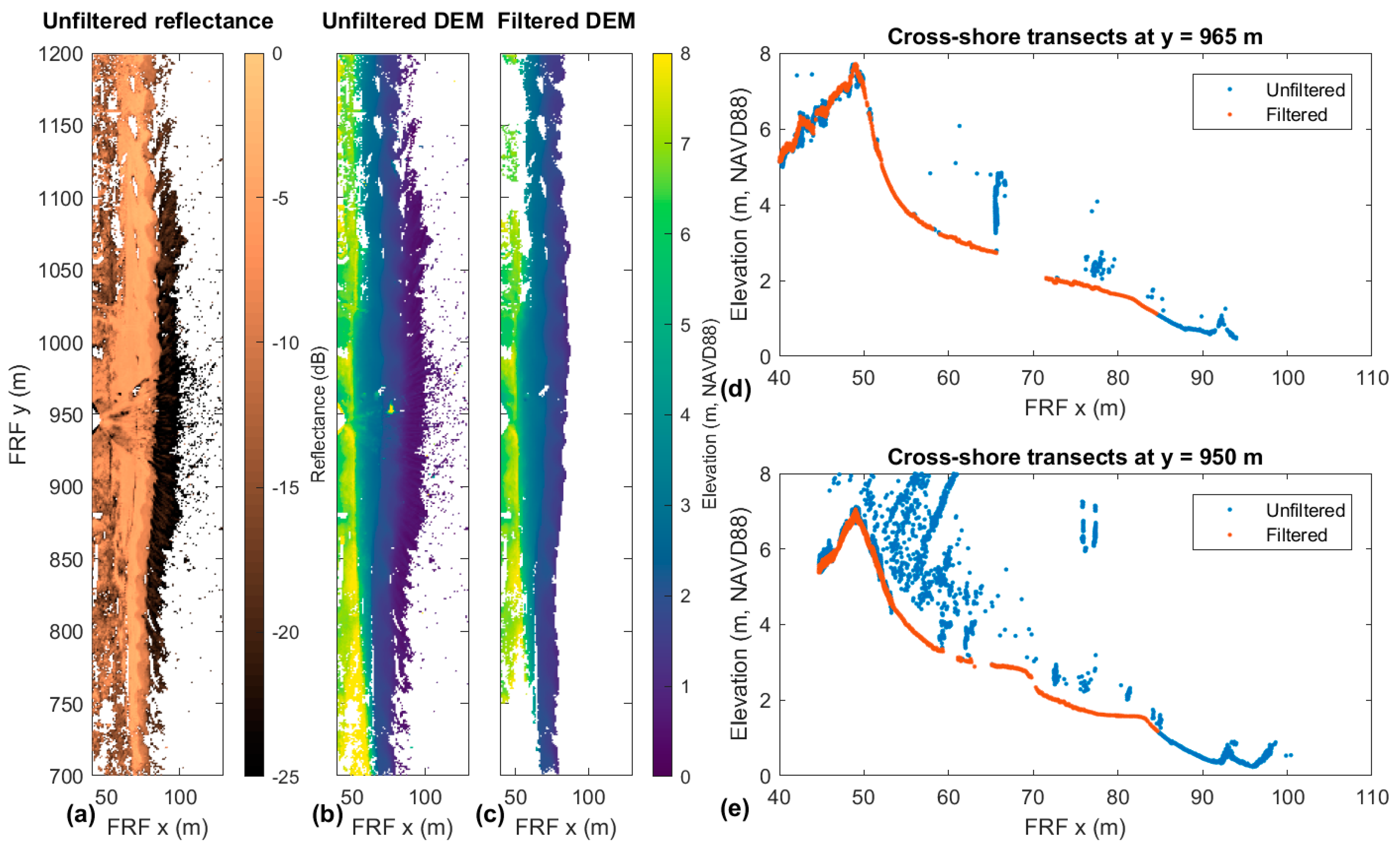
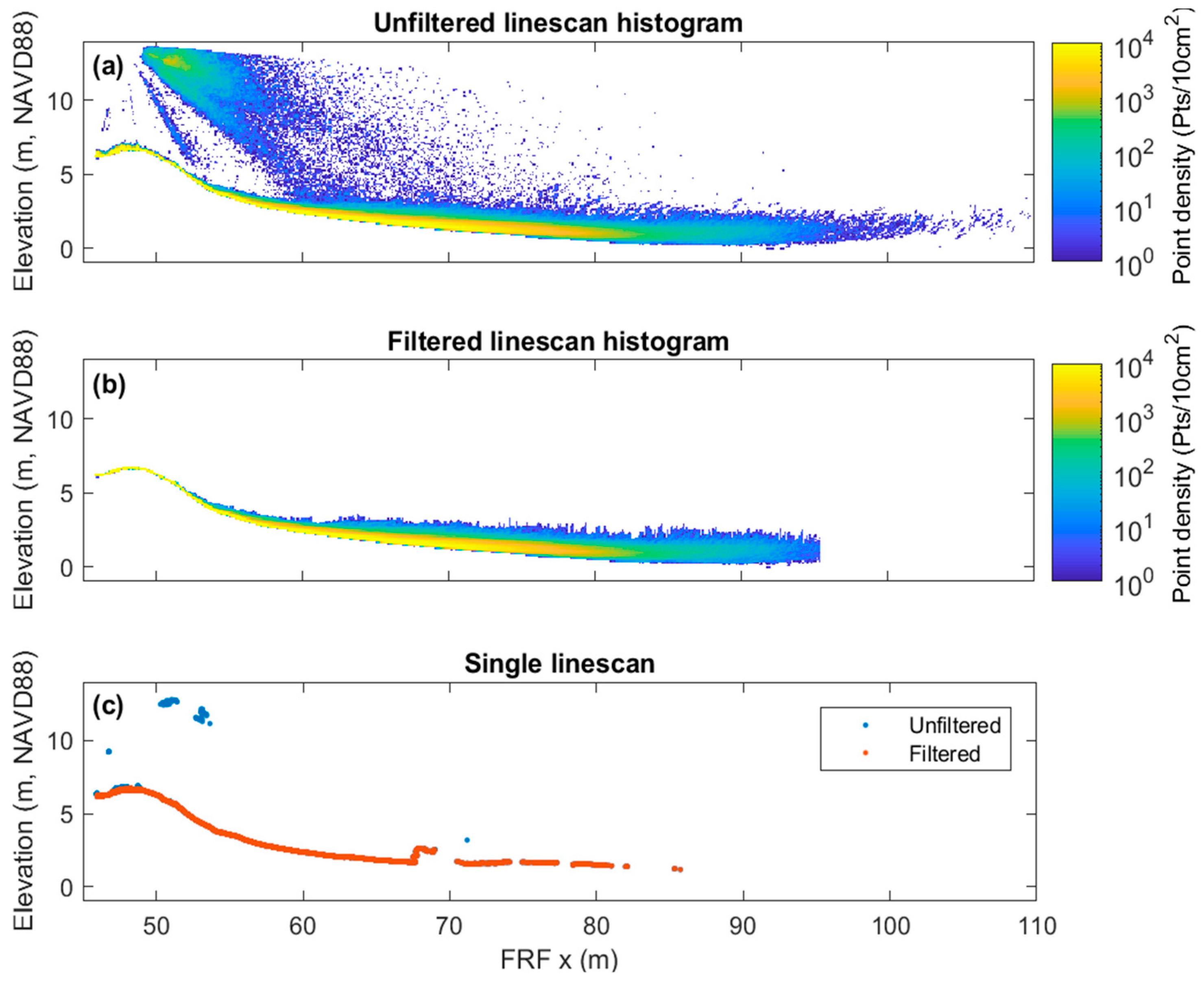
2.3.3. Scan Filtering
2.3.4. Point Cloud Gridding
3. Results: Data Products
3.1. Runup
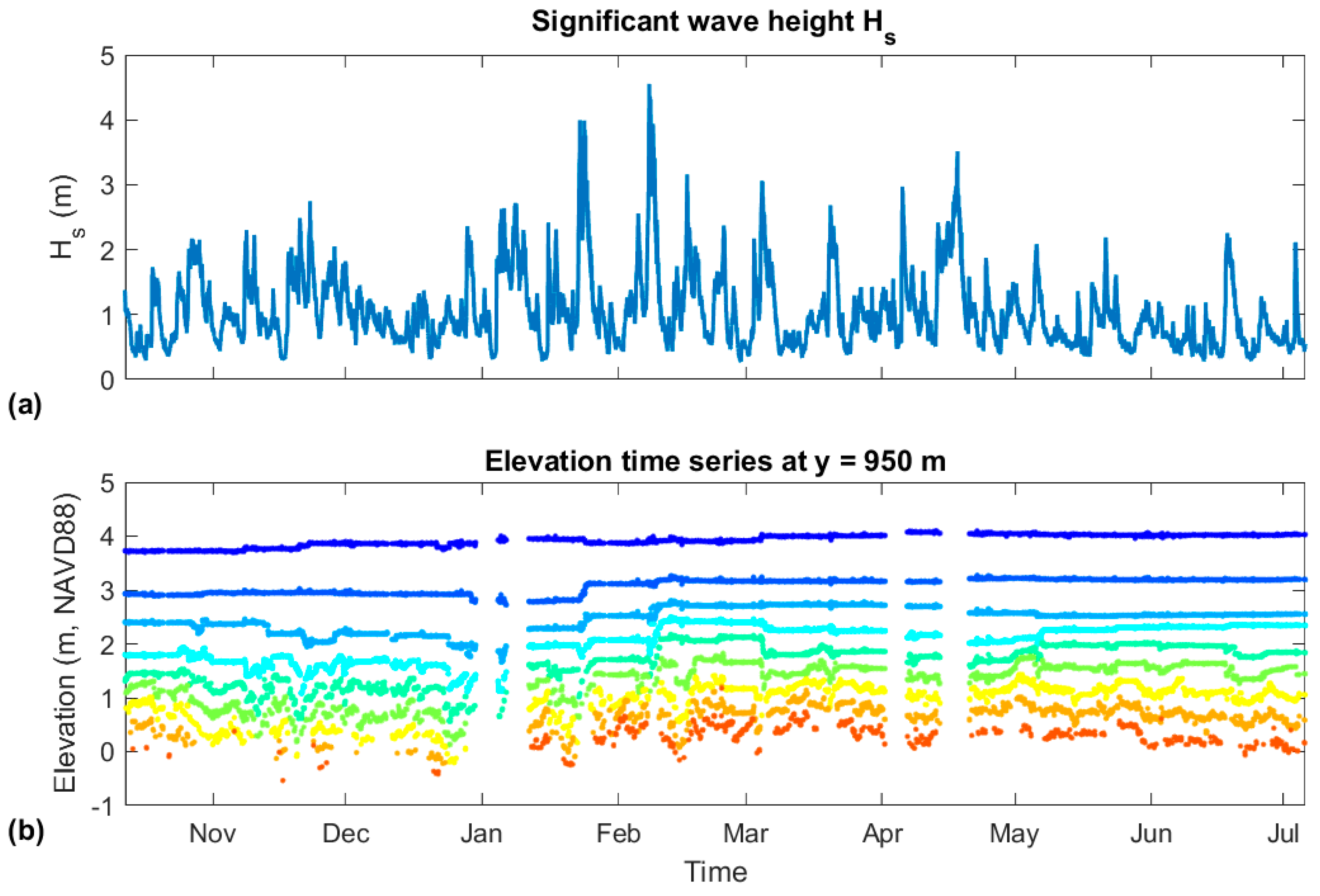
3.2. Hydrodynamics
3.3. Morphology
4. Discussion
4.1. Applications
4.1.1. Long (Seasonal to Annual) Time Scales
4.1.2. Event Scales
4.1.3. Short (Wave-by-Wave) Time Scales
4.2. Error Propagation
5. Conclusions
Author Contributions
Funding
Acknowledgments
Conflicts of Interest
References
- Holman, R.A.; Stanley, J. The history and technical capabilities of Argus. Coast. Eng. 2007, 54, 477–491. [Google Scholar] [CrossRef]
- Birkemeier, W.E.; Thorton, E.B. The DUCK94 Nearshore Field Experiment. In Proceedings of the Coastal Dynamics 1994 Conference, Barcelona, Spain, 21–25 February 1994; Arcilla, A.C., Marcel, S.J.F., Kraus, N.C., Eds.; American Society of Civil Engineers: New York, NY, USA, 1994; pp. 815–821. [Google Scholar]
- Turner, I.L.; Harley, M.D.; Short, A.D.; Simmons, J.A.; Bracs, M.A.; Phillips, M.S.; Splinter, K.D. A multi-decade dataset of monthly beach profile surveys and inshore wave forcing at Narabeen, Australia. Sci. Data 2016, 3, 160024. [Google Scholar] [CrossRef] [PubMed]
- Holman, R.A.; Haller, M.C. Remote Sensing of the Nearshore. Annu. Rev. Mar. Sci. 2013, 5, 95–113. [Google Scholar] [CrossRef] [PubMed]
- Holman, R.; Stanley, J.; Özkan-Haller, T. Applying video sensor networks to nearshore environment monitoring. IEEE Pervasive Comput. 2003, 2, 14–21. [Google Scholar] [CrossRef]
- Lippmann, T.C.; Holman, R.A. The spatial and temporal variability of sand bar morphology. J. Geophys. Res. 1990, 95, 11575–11590. [Google Scholar] [CrossRef]
- Holman, R.A.; Symonds, G.; Thornton, E.B.; Ranasinghe, R. Rip spacing and persistence on an embayed beach. J. Geophys. Res. Ocean. 2006, 111, C01006. [Google Scholar] [CrossRef]
- Ranasinghe, R.; Holman, R.; de Schipper, M.; Lippmann, T.; Wehof, J.; Duong, T.M.; Roelvink, D.; Stive, M. Quantifying nearshore morphological recovery time scales using argus video imaging: Palm Beach, Sydney and Duck, North Carolina. In Proceedings of the 33rd Conference on Coastal Engineering, Santander, Spain, 1–6 July 2012. [Google Scholar]
- Holman, R.; Plant, N.; Holland, T. CBathy: A robust algorithm for estimating nearshore bathymetry. J. Geophys. Res. Ocean. 2013, 118, 2595–2609. [Google Scholar] [CrossRef]
- Plant, N.G.; Holman, R.A. Intertidal beach profile estimation using video images. Mar. Geol. 1997, 140, 1–24. [Google Scholar] [CrossRef]
- Chickadel, C.C.; Holman, R.A.; Freilich, M.H. An optical technique for the measurement of longshore currents. J. Geophys. Res. 2003, 108, 3364. [Google Scholar] [CrossRef]
- Stockdon, H.F.; Holman, R.A.; Howd, P.A.; Sallenger, A.H. Empirical parameterization of setup, swash, and runup. Coast. Eng. 2006, 53, 573–588. [Google Scholar] [CrossRef]
- Pianca, C.; Holman, R.; Siegle, E. Shoreline variability from days to decades: Results of long-term video imaging. J. Geophys. Res. Ocean. 2015, 120, 2159–2178. [Google Scholar] [CrossRef]
- Brock, J.C.; Purkis, S.J. The Emerging Role of Lidar Remote Sensing in Coastal Research and Resource Management. J. Coast. Res. Spec. Issue 2009, 10053, 1–5. [Google Scholar] [CrossRef]
- Wang, Y. (Ed.) Remote Sensing of Coastal Environments; CRC Press: Boca Raton, FL, USA, 2010. [Google Scholar]
- Klemas, V. Beach Profiling and LIDAR Bathymetry: An Overview with Case Studies. J. Coast. Res. 2011, 27, 1019–1028. [Google Scholar] [CrossRef]
- Brodie, K.L.; Spore, N.J. Foredune classification and storm response: Automated analysis of terrestrial lidar DEMs. In Proceedings of the Coastal Sediments 2015, San Diego, CA, USA, 11–15 May 2015; Wang, P., Rosati, J., Cheng, J., Eds.; World Scientific Publishing Company: Singapore, 2015. [Google Scholar]
- Sallenger, A.H., Jr.; Krabill, W.B.; Swift, R.N.; Brock, J.; List, J.; Hansen, M.; Holman, R.A.; Manizade, S.; Sontag, J.; Meredith, A.; et al. Evaluation of airborne topographic lidar for quantifying beach changes. J. Coast. Res. 2003, 19, 125–133. [Google Scholar]
- National Oceanic and Atmospheric Administration (NOAA) Coastal Services Center. Lidar 101: An Introduction to Lidar Technology, Data, and Applications; Revised; NOAA Coastal Services Center: Charleston, SC, USA, 2012.
- Pietro, L.S.; O’Neal, M.A.; Puleo, J.A. Developing Terrestrial-LIDAR-Based Digital Elevation Models for Monitoring Beach Nourishment Performance. J. Coast. Res. 2008, 24, 1555–1564. [Google Scholar] [CrossRef]
- Young, A.P.; Olsen, M.J.; Driscoll, N.; Flick, R.E.; Gutierrez, R.; Guza, R.T.; Johnstone, E.; Kuester, F. Comparison of Airborne and Terrestrial Lidar Estimates of Seacliff Erosion in Southern California. Photogramm. Eng. Remote Sens. 2010, 76, 421–427. [Google Scholar] [CrossRef]
- Corbí, H.; Riquelme, A.; Megías-Baños, C.; Abellan, A. 3-D morphological change analysis of a beach with seagrass berm using a terrestrial laser scanner. ISPRS Int. J. Geo-Inf. 2018, 7, 234. [Google Scholar]
- Saye, S.E.; van der Wal, D.; Pye, K.; Blott, S.J. Beach-dune morphological relationships and erosion/accretion: An investigation at five sites in England and Wales using LIDAR data. Geomorphology 2005, 72, 128–155. [Google Scholar] [CrossRef]
- Revell, D.L.; Komar, P.D.; Sallenger, A.H. An application of LIDAR to analyses of El Nino erosion in the Netarts littoral cell, Oregon. J. Coast. Res. 2002, 18, 792–801. [Google Scholar]
- Donker, J.; van Maarseveen, M.; Ruessink, G. Spatio-Temporal Variations in Foredune Dynamics Determined with Mobile Laser Scanning. J. Mar. Sci. Eng. 2018, 6, 126. [Google Scholar] [CrossRef]
- Blenkinsopp, C.E.; Mole, M.A.; Turner, I.L.; Peirson, W.L. Measurements of the time varying free-surface profile across the swash zone obtained using an industrial LiDAR. Coast. Eng. 2010, 57, 1059–1065. [Google Scholar] [CrossRef]
- Almeida, L.P.; Masselink, G.; Russell, P.; Davidson, M.; Poate, T.; McCall, R.; Blenkinsopp, C.; Turner, I. Observations of the swash zone on a gravel beach during a storm using a laser-scanner (Lidar). J. Coast. Res. Spec. Issue 2013, 65, 636–641. [Google Scholar] [CrossRef]
- Brodie, K.L.; Raubenheimer, B.; Elgar, S.; Slocum, R.K.; McNinch, J.E. Lidar and pressure measurements of inner-surfzone waves and setup. J. Atmos. Ocean. Technol. 2015, 32, 1945–1959. [Google Scholar] [CrossRef]
- Martins, K.; Blenkinsopp, C.E.; Power, H.E.; Bruder, B.; Puleo, J.A.; Bergsma, E.W. High resolution monitoring of wave transformation in the surf zone using a LiDAR scanner array. Coast. Eng. 2017, 128, 37–43. [Google Scholar] [CrossRef]
- Martins, K.; Blenkinsopp, C.E.; Deigaard, R.; Power, H.E. Energy dissipation in the inner surf zone: New insights from LiDAR-based roller geometry measurements. J. Geophys. Res. Ocean. 2018, 123, 3386–3407. [Google Scholar] [CrossRef]
- Almeida, L.P.; Masselink, G.; Russell, P.; Davidson, M. Observations of gravel beach dynamics during high energy wave conditions using a laser scanner. Geomorphology 2015, 228, 15–27. [Google Scholar] [CrossRef]
- Schubert, J.E.; Gallien, T.W.; Majd, M.S.; Sanders, B.F. Terrestrial laser scanning of anthropogenic beach berm erosion and overtopping. J. Coast. Res. 2015, 31, 47–60. [Google Scholar] [CrossRef]
- LeWinter, A.L.; Finnegan, D.C.; Hamilton, G.S.; Stearns, L.A.; Gadomski, P.J. Continuous monitoring of Greenland outlet glaciers using an autonomous terrestrial LiDAR scanning system: Design, development and testing at Helheim Glacier. In Proceedings of the American Geophysical Union Fall Meeting 2014, San Francisco, CA, USA, 12–16 December 2014. Abstract C31B-0292. [Google Scholar]
- Splinter, K.D.; Harley, M.D.; Turner, I.L. Remote sensing is changing our view of the coast: Insights from 40 years of monitoring at Narabeen-Collaroy, Australia. Remote Sens. 2018, 10, 1744. [Google Scholar] [CrossRef]
- Mason, C.; Birkemeier, W.A.; Howd, P.A. An Overview of DUCK85, a Nearshore Processes Experiment. In Proceedings of the Coastal Sediments ’87 Conference, ASCE, New Orleans, LA, USA, 12–13 May 1987. [Google Scholar]
- Crowson, R.A.; Birkemeier, W.A.; Klein, H.M.; Miller, H.C. SUPERDUCK Nearshore Processes Experiment: Summary of Studies, CERC Field Research Facility; Technical Report CERC-88-12; US Army Engineer Waterways Experiment Station: Vicksburg, MS, USA, 1988. [Google Scholar]
- Birkemeier, W.A.; Donoghue, C.; Long, C.E.; Hathaway, K.K.; Baron, C.F. The DELILAH Nearshore Experiment: Summary Data Report; US Army Corps of Engineers, Waterways Experiment Station: Vicksburg, MS, USA, 1997. [Google Scholar]
- Hartzell, P.J.; Gadomski, P.J.; Glennie, C.L.; Finnegan, D.C.; Deems, J.S. Rigorous error propagation for terrestrial laser scanning with application to snow volume uncertainty. J. Glaciol. 2015, 61, 1147–1158. [Google Scholar] [CrossRef]
- Zhang, W.; Qi, J.; Wan, P.; Wang, H.; Xie, D.; Wang, X.; Yan, G. An Easy-to-Use Airborne LiDAR Data Filtering Method Based on Cloth Simulation. Remote Sens. 2016, 8, 501. [Google Scholar] [CrossRef]
- Holman, R.A.; Sallenger, A.H. Setup and Swash on a Natural Beach. J. Geophys. Res. 1985, 90, 945–953. [Google Scholar] [CrossRef]
- Komar, P.D. Beach Processes and Sedimentation; Prentice-Hall: Upper Saddle River, NJ, USA, 1998; 544p. [Google Scholar]
- Elgar, S.; Guza, R.T. Observations of bispectra of shoaling surface gravity waves. J. Fluid Mech. 1985, 161, 425–448. [Google Scholar] [CrossRef]
- Roelvink, D.; Reniers, A.; van Dongeren, A.; van Thiel de Vries, J.; McCall, R.; Lescinski, J. Modelling storm impacts on beaches, dunes and barrier islands. Coast. Eng. 2009, 56, 1133–1152. [Google Scholar] [CrossRef]
- Palmsten, M.L.; Holman, R.A. Laboratory investigation of dune erosion using stereo video. Coast. Eng. 2012, 60, 123–135. [Google Scholar] [CrossRef]
- Stockdon, H.F.; Thompson, D.M.; Plant, N.G.; Long, J.W. Evaluation of wave runup predictions from numerical and parametric models. Coast. Eng. 2014, 92, 1–11. [Google Scholar] [CrossRef]
- Overbeck, J.R.; Long, J.W.; Stockdon, H.F. Testing model parameters for wave-induced dune erosion using observations from Hurricane Sandy. Geophys. Res. Lett. 2017, 44, 937–945. [Google Scholar] [CrossRef]
- Fiedler, J.W.; Brodie, K.L.; McNinch, J.E.; Guza, R.T. Observations of runup and energy flux on a low-slope beach with high-energy, long-period ocean swell. Geophys. Res. Lett. 2015, 42, 9933–9941. [Google Scholar] [CrossRef]
- Elgar, S.; Gallagher, E.L.; Guza, R.T. Nearshore sandbar migration. J. Geophys. Res. Ocean. 2001, 106, 11623–11627. [Google Scholar] [CrossRef]
- García-Medina, G.; Özkan-Haller, H.T.; Holman, R.A.; Ruggiero, P. Large runup controls on a gently sloping dissipative beach. J. Geophys. Res. Ocean. 2017, 122, 5998–6010. [Google Scholar] [CrossRef]
- Ruggiero, P.; Holman, R.A.; Beach, R.A. Wave run-up on a high-energy dissipative beach. J. Geophys. Res. C Ocean. 2004, 109, C06025. [Google Scholar] [CrossRef]
- Holland, K.T.; Holman, R.A. Video estimation of foreshore topography using trinocular stereo. J. Coast. Res. 1997, 13, 81–87. [Google Scholar]
- Butt, T.; Russell, P. Hydrodynamics and cross-shore sediment transport in the swash-zone of natural beaches: A review. J. Coast. Res. 2000, 16, 255–268. [Google Scholar]
- Puleo, J.A.; Beach, R.A.; Holman, R.A.; Allen, J.S. Swash zone sediment suspension and transport and the importance of bore-generated turbulence. J. Geophys. Res. Ocean. 2000, 105, 17021–17044. [Google Scholar] [CrossRef]
- Butt, T.; Russell, P.; Puleo, J.; Miles, J.; Masselink, G. The influence of bore turbulence on sediment transport in the swash and inner surf zones. Cont. Shelf Res. 2004, 24, 757–771. [Google Scholar] [CrossRef]
- Masselink, G.; Puleo, J.A. Swash-zone morphodynamics. Cont. Shelf Res. 2006, 26, 661–680. [Google Scholar] [CrossRef]
- Turner, I.L.; Russell, P.E.; Butt, T. Measurement of wave-by-wave bed-levels in the swash zone. Coast. Eng. 2008, 55, 1237–1242. [Google Scholar] [CrossRef]
- Masselink, G.; Russell, P.; Turner, I.; Blenkinsopp, C. Net sediment transport and morphological change in the swash zone of a high-energy sandy beach from swash event to tidal cycle time scales. Mar. Geol. 2009, 267, 18–35. [Google Scholar] [CrossRef]
- Blenkinsopp, C.E.; Turner, I.L.; Masselink, G.; Russell, P.E. Swash zone sediment fluxes: Field observations. Coast. Eng. 2011, 58, 28–44. [Google Scholar] [CrossRef]
- Puleo, J.A.; Lanckriet, T.; Blenkinsopp, C. Bed level fluctuations in the inner surf and swash zone of a dissipative beach. Mar. Geol. 2014, 349, 99–112. [Google Scholar] [CrossRef]
- Vousdoukas, M.I.; Kirupakaramoorthy, T.; Oumeraci, H.; de la Torre, M.; Wübbold, F.; Wagner, B.; Schimmels, S. The role of combined laser scanning and video techniques in monitoring wave by-wave swash zone processes. Coast. Eng. 2014, 83, 150–165. [Google Scholar] [CrossRef]


© 2019 by the authors. Licensee MDPI, Basel, Switzerland. This article is an open access article distributed under the terms and conditions of the Creative Commons Attribution (CC BY) license (http://creativecommons.org/licenses/by/4.0/).
Share and Cite
O’Dea, A.; Brodie, K.L.; Hartzell, P. Continuous Coastal Monitoring with an Automated Terrestrial Lidar Scanner. J. Mar. Sci. Eng. 2019, 7, 37. https://doi.org/10.3390/jmse7020037
O’Dea A, Brodie KL, Hartzell P. Continuous Coastal Monitoring with an Automated Terrestrial Lidar Scanner. Journal of Marine Science and Engineering. 2019; 7(2):37. https://doi.org/10.3390/jmse7020037
Chicago/Turabian StyleO’Dea, Annika, Katherine L. Brodie, and Preston Hartzell. 2019. "Continuous Coastal Monitoring with an Automated Terrestrial Lidar Scanner" Journal of Marine Science and Engineering 7, no. 2: 37. https://doi.org/10.3390/jmse7020037