Article

Reduced Order Data-Driven Analysis of Cavitating Flow over Hydrofoil with Machine Learning

1
College of Water Resources and Civil Engineering, China Agricultural University, Beijing 100083, China
2
State Grid Henan Electric Power Research Institute, Zhengzhou 450052, China
3
College of Information and Electrical Engineering, China Agricultural University, Beijing 100083, China
*
Author to whom correspondence should be addressed.
J. Mar. Sci. Eng. 2024, 12(1), 148; https://doi.org/10.3390/jmse12010148
Submission received: 30 November 2023 / Revised: 4 January 2024 / Accepted: 10 January 2024 / Published: 12 January 2024
(This article belongs to the Special Issue Advancement in the Multiphase Flow in Fluid Machinery)

Abstract

:
Predicting the flow situation of cavitation owing to its high-dimensional nonlinearity has posed great challenges. To address these challenges, this study presents a novel reduced order modeling (ROM) method to accurately analyze and predict cavitation flow fields under different conditions. The proposed ROM decomposes the flow field into linearized low-order modes while maintaining its accuracy and effectively reducing its dimensionality. Specifically, this study focuses on predicting cavitation on the Clark-Y hydrofoil using a combination of numerical simulation, proper orthogonal decomposition (POD), and neural networks. By analyzing different cavitation conditions, the results revealed that the POD method effectively reduces the order of the cavity flow field while achieving excellent flow field reconstruction. Notably, the zeroth- and first-order modes are associated with attachment cavitation, while the second-, third- and fourth-order modes correspond to cavitation shedding. Additionally, the fifth- and sixth-order modes along the hydrofoil surface are associated with the backward jet flow. To predict the conditions of high-energy modes, the neural network proved to be more effective, exhibiting excellent performance in stable attached cavitation. However, for cloud cavitation, the accuracy of the neural network model requires further improvement. This study not only introduces a novel approach for predicting cavitation flow fields but also highlights new challenges that will require continuous attention in future research endeavors.

1. Introduction

Cavitation is an inevitable problem when studying flow in liquid media [1]. This problem becomes more pronounced when using pumps, turbines, or hydro-turbines to transport liquid media or generate power, as drastic changes in pressure can trigger cavitation [2,3,4,5]. Cavitation leads to several adverse effects, such as noise [6], vibration [7], and material damage [8]. Its presence has far-reaching consequences across various fields, such as aerospace (liquid hydrogen and liquid oxygen transportation) [9], ocean energy utilization (tidal, ocean current, and wave energy conversion) [10], hydraulic engineering (water transportation) [11], hydropower (water energy utilization) [12], and ships (propeller problem) [13]. As cavitation can cause performance degradation and material damage in fluid machinery, it poses a great risk to operational safety and stability [14,15].
Hydrofoils serve as simplified models of fluid machinery blades and are commonly used to simplify the complex internal flow of impellers; therefore, they are widely used in basic research in fluid machinery and engineering [16,17]. To investigate hydrodynamic cavitation, researchers often use a cavitation water tunnel, where various foil profiles are installed and tested [18]. By adjusting the flow rate of the circulating pump and valves, the speed of upstream flow can be altered, and different cavitation states can be investigated by controlling the environmental pressure through adjustments to the vacuum pump and cavitation tank. Researchers have extensively studied different states of hydrofoil cavitation. On smaller cavitation scales, it exhibits an attached and relatively stable state [19,20]. As the cavitation scales increase, the cavities become unstable and shed along the flow direction [21,22,23]. When cavitation encompasses the entire flowing object, it is termed supercavitation, characterized by unique fluid dynamics [24]. Additionally, in cases with a gap at the end, tip leakage cavitation may occur, which has attracted the attention of numerous researchers [25,26]. Overall, the cavitation flow field is characterized by high-dimensional nonlinearity [27,28]. Its varied forms and complexities under different situations pose great challenges for research endeavors.
In reality, the complex changes in cavitation are closely related to turbulent flow [29]. Turbulence was first observed by Reynolds, who noticed the transition of flow in a circular tube from regular to turbulent as the incoming flow velocity increased. However, the Navier–Stokes equation, when averaged, faces closure problems, and the existence and smoothness of the equation remain unresolved [30,31]. Fortunately, with advancements in science and technology, numerical solutions for turbulence have played a significant role, leading to notable progress in turbulence research [32,33,34]. This progress can be attributed to the efforts of researchers such as Prandtl, who addressed practical problems in fluid mechanics. The large amount of data generated, including experimental, simulation, and image data, can potentially supplement and improve the missing and unresolved turbulence control equations if adequately processed and summarized [35]. Although this remains challenging, summarizing the statistical laws in massive data through data-driven approaches aligns with the efforts of researchers such as Taylor and von Carmen.
Currently, machine learning plays a crucial role in handling massive amounts of data, significantly advancing the field of fluid dynamics. Some scholars have also conducted research on how machine learning can be applied in the field of fluid machinery [36]. However, handling large amounts of data presents a great challenge, particularly when considering the application of machine learning techniques. To effectively use machine learning, it becomes essential to implement functions such as dimensionality reduction [37] and sparse identification [38] and then achieve temporal or spatial prediction [39]. The most commonly used method for reducing the dimensionality of complex dynamic flow systems is linear mode decomposition. It separates the spatiotemporal coherent structural features of the flow field in low-dimensional space [40,41]. This approach decomposes the high-dimensional flow field into a linear superposition of lower-order modes containing principal components with specific physical significance. By analyzing these lower-order modes individually, richer and more specific information can be extracted from the overall flow. Another frequently used method is proper orthogonal decomposition (POD), which decomposes a random quantity into a set of basis functions determined by its own characteristics to represent it [42]. In POD, the principle for determining the basis function is to maximize the energy on the lowest order pattern during each decomposition process. Dynamic mode decomposition (DMD) is another method of flow field feature extraction [43]. It focuses on frequency analysis and offers a unique advantage in spatiotemporal coupling modeling. Compared to DMD, the POD method analyzes the flow field from an energy perspective and has better adaptability in flow field analysis.
Several researchers have applied the POD method in flow field analysis. Liberge et al. [44] investigated the flow around an oscillating cylinder using POD and constructed a low-order dynamic system to characterize flow features. Xie et al. [45] conducted POD of the flow field inside a bending duct, extensively reconstructing and analyzing the Karman vortex street and other vortex characteristics. Liu et al. [46] extracted the dominant modes of the flow field around ALE 15 hydrofoil. They extensively explored the characteristics of the hydrofoil-surrounded flow field and compared the POD with other mode decomposition methods. Wu et al. [47] studied the flow inside the jet pipe using POD and demonstrated the coherent structure of the flow with the snapshot POD technique. Resseguier et al. [48] introduced a random model based on the POD, which improved the accuracy and stability of small-scale turbulent flow analysis. Although POD has gained wide applications, challenges persist in the mode decomposition of two-phase flow fields, mainly arising from the complexity of flow field information (discussed in the next chapter) [49]. This complexity presents obstacles to machine learning and requires further exploration.
This study focuses on the computational fluid dynamics analysis of the cavitation flow field around the classic Clark-Y hydrofoil [50]. The validity of the data is verified through comparison with experimental data. The POD is then used to attempt dimensionality reduction in the convection field at a certain cavitation number (within the range of cavitation scale and morphology). It aims to summarize the data information rules from different orders, effectively combining neural networks to explore machine learning possibilities and discuss the potential of breaking away from tedious computational fluid dynamics processes. Additionally, the results of this study provide scientific support for a deeper understanding of the mechanism of hydrofoil shedding cavitation.

2. Hydrofoil Cavitation Problem

Cavitation is a liquid–gas phase transition that occurs at the edge of the gas–liquid phase saturation state. Figure 1 shows the phase diagram of the cavitation process. If the temperature remains constant and the pressure p drops below the saturation pressure pv, the liquid–gas phase transition is generally referred to as ‘cavitation’:
p < p v ,
Conversely, if the pressure remains constant and the temperature rises, it is referred to as ‘boiling’. Despite their different names, the two processes have the same mechanism.
For cavitation over a hydrofoil, the position of the lowest pressure point or low-pressure zone determines the location of cavitation. Figure 2 shows that when the hydrofoil is at a certain incidence angle, the incoming flow collides with the high-pressure side of the foil while the opposite side experiences low pressure. Slightly downstream from the flow separation point lies the lowest pressure point, corresponding to a certain range of the lowest pressure region. If the flow regime in the low-pressure region remains stable, cavitation occurs in an attached state. However, as the environmental pressure decreases or the incidence angle changes, the low-pressure region expands to areas of unstable flow. At this point, the cavitation enters a shedding state, and the shedding vortex core is characterized by very low pressure with cavitation inside. If the low pressure continues to increase, super cavitation occurs, and the entire foil is surrounded by cavities.
If a monitoring point is placed on the surface of the hydrofoil, such as the MP0 point in Figure 2, the pressure variation at this point typically exhibits periodic fluctuations when cavitation does not occur (i.e., pressure is high). Figure 3 shows that the fluctuation pattern is relatively smooth and continuous. However, during shedding cavitation, the vapor volume fraction fv at the MP0 point exhibits pulsations. The fv pulsation is bounded between 0 and 1, resulting in a ‘ceiling’ limitation that poses great challenges in investigating the cavitating flow [51]. Therefore, there is a pressing need to acquire more mathematical and physical information through data-driven approaches.

3. Simulation Data Preparation

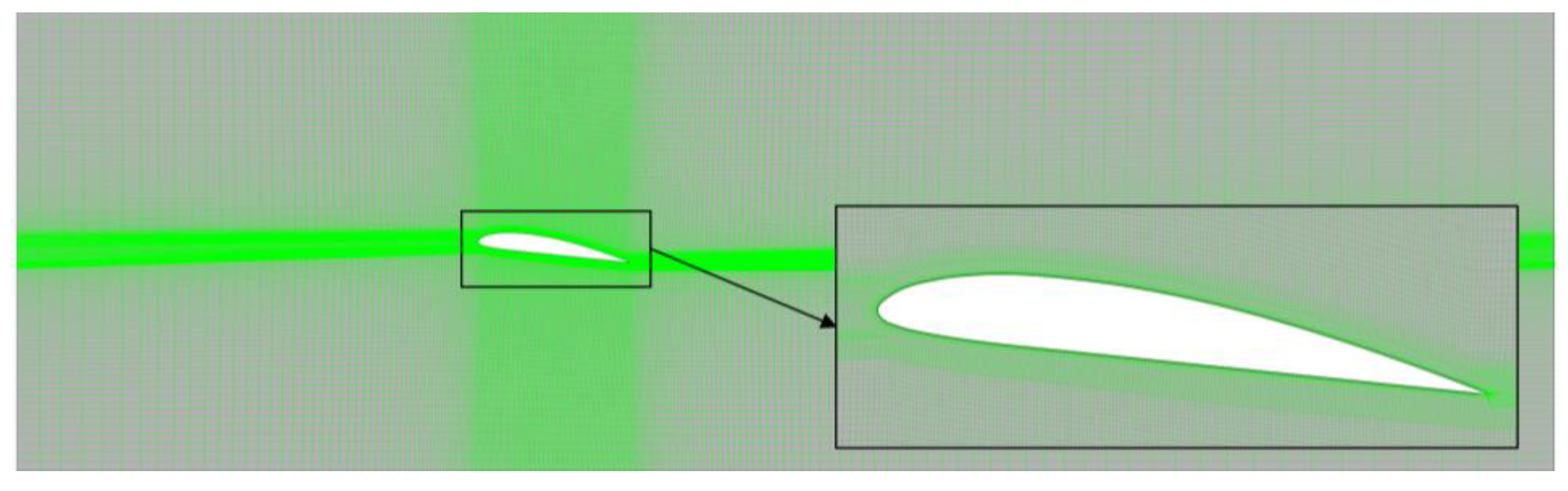
3.1. Clark-Y Hydrofoil Model and Flow Field Discretization

In this study, the case of the Clark-Y hydrofoil model is used to examine the characteristics of surface low-pressure region cavitation and its shedding behavior [49]. Figure 4 shows the computational domain, and the specific values of each linear dimension are presented in Table 1. Additionally, the chord length c, maximum thickness tbmax, and incidence angle α of hydrofoil are shown in Figure 4 and presented in Table 1.

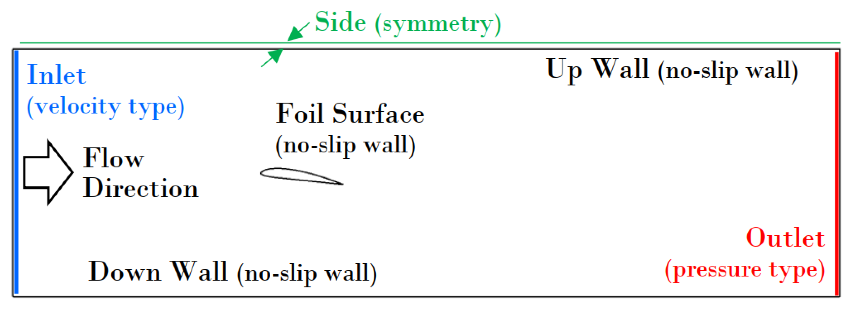
3.2. Setup of Computational Fluid Dynamics

Computational fluid dynamics (CFD) is used to simulate the cavitation phenomenon. Two phases of water and steam are considered for the medium at 20 °C within the computational domain. The boundary conditions are designed to meet the simulation requirements, as shown in Figure 5. The inlet is a velocity inlet with a value of 10 m/s., while the outlet is a static pressure outlet that can be adjusted to simulate different cavitation scenarios. The surface of the hydrofoil is treated as a boundary of the no-slip wall type, and the upper and lower boundaries of the domain follow the same no-slip wall type. Symmetry-type boundaries are used to simplify 3D calculations to 2D and reduce computational costs. The turbulent flow is modeled using the shear stress transport model [35,52], while the cavitation mass transfer uses the Zwart model [53]. Figure 6 shows the mesh used in the CFD simulation. After boundary refinement, the 2D mesh has a total of 112,896 nodes with a y+ value of approximately 1.0.
In this study, two dimensionless parameters are important: the Reynolds and cavitation numbers. They can be expressed as follows:
R e = ρ v i n c μ
σ = 2 ( p i n p v ) ρ v i n 2
where ρ is the density, vin is the inlet velocity, c is the foil chord length, μ is the dynamic viscosity, pin is the inlet pressure, and pv is the saturation pressure. In this study, the Reynolds number used is 6.9 × 10⁵, and the cavitation number ranges from 0.59 to 0.96, with an increment of 0.01 for each operating condition.

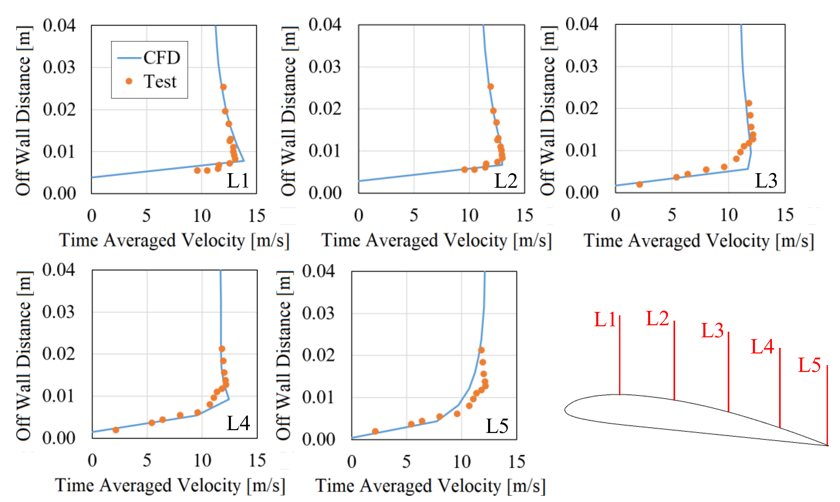
3.3. Verification and Validation of Simulation Data

To verify the accuracy of the CFD convection field prediction, a comparative analysis was conducted between CFD data and test data [49] at a cavitation number σ = 0.8, as shown in Figure 7. The main focus was on comparing the distribution of time-averaged velocity off the wall at five different positions on the hydrofoil surface. The results reveal that the predicted CFD velocity values and test values are in strong agreement at these five different positions, reflecting the high predictive performance of the CFD simulation for the flow field. This validation confirms the suitability of the data for smooth modal decomposition and machine learning. Figure 8 shows the vapor volume distribution at different cavitation numbers during the same time step. As the cavitation number decreases from σ = 0.96 to σ = 0.59, the volume of cavitation gradually increases, and the covered area expands downstream, showing a trend of downstream shedding of the cavity. Additionally, within the range shown in Figure 8, the cavity length increases from 70% to 100% of the hydrofoil length.

4. Order Reduction in Cavitating Flow Data

4.1. Proper Orthogonal Decomposition

As previously mentioned, POD is a reduced order method based on singular value decomposition. When applied to flow field analysis, especially spatial high-resolution flow field analysis obtained through simulation, POD samples data from different time points. Based on this, the flow field information f is decomposed into spatially correlated orthogonal bases and can be expressed as follows:
f = [ | f ( t 1 ) | | f ( t 2 ) | L | f ( t n ) | ] ,
where the column of f(ti) is the ith flow field snapshot. Before solving the POD mode, it is customary to subtract the average value of the flow field and split the snapshot into two parts: the mean and pulsation. The mean part is referred to as the zeroth-order mode, while the pulsation part is decomposed to obtain the first-, second-, …, nth-order modes as follows:
f = U Σ V T = j = 1 r σ j u j v j T ,
where r is the rank of matrix f. U is the orthogonal matrix column of uj, with a size of n × r. V is the orthogonal matrix column of vj, with a size of m × r. Σ, the singular value representing the scaling relationship between U and V, is the diagonal matrix of size r × r and it is referred to as the ‘energy’ of modes. After decomposing the flow field, if the first nth-order modes with high energy can effectively reconstruct the information of the original flow field (with an error less than a specific proportion), then these modes are referred to as the dominant modes. This enables the flow field to be effectively split and analyzed, laying the foundation for subsequent machine learning analysis.

4.2. Flow Pattern by Order

Figure 9 and Figure 10 show the analysis of the time step of cavitation shedding under σ = 0.8 conditions. In Figure 9, the POD decomposition results indicate the energy proportion of the first 10 orders, excluding the mean field of the 0th order. The first mode exhibits the highest energy and accounts for over 40% of the total energy, while the second and third modes also exceed 10% energy contribution. The energy of subsequent modes gradually decreases. From the perspective of accumulated energy, the sum of the first six orders exceeds an 80% criterion, making them the dominant modes with great influence on the flow behavior. Figure 10 shows the specific image situation for various modes. Comparing the modes with the general field, it becomes evident that the strongest point of the mean field corresponds to the stable cavitation position at the leading-edge and front part of the hydrofoil, with the first mode also dominating at this position. The second-, third-, and fourth-order modes are most prominent at the trailing edge, representing the shedding of cavitation. Additionally, the fifth and sixth modes exhibit changes on the surface of the hydrofoil, indicating the flow of fluid along the foil surface.

4.3. Energy Law of Modes

Examining the changes in the proportion of energy in different modes is important for data-driven research. Figure 11a shows an analysis of the energy proportion of the first to sixth-order modes as a function of the cavitation number σ. Overall, the energy intensity of the first- and second-order modes decreases as σ increases, while the other orders show an opposite trend. Using linear fitting analysis, the formula obtained is expressed as follows:
E M = C 0 + C 1 σ ,
where C0 is a constant term, C1 is a first-order term, and EM is the proportion of energy of modes. Figure 11b shows the law of the first-order term C1 in linear fitting. As the cavitation scale increases with the rising σ, the attached cavitation at the leading edge becomes stronger, while the shedding cavitation at the trailing edge weakens.

5. Learning and Prediction

5.1. Workflow

In an attempt to learn and predict cavitation flow fields, a workflow combining neural networks and POD is used, as shown in Figure 12. The process involves data collection, neural network training, and prediction. The data used are generated through CFD simulation of the flow field, especially the flow field data of the cavitation vapor volume fraction. Based on these data, a database is constructed for the different cavitation number conditions. In this study, the backpropagation (BP) neural network is used, and the data are divided into training, testing, and validation sets, with approximately 70% of samples used for training, 15% for testing, and 15% for validation. The Levenberg–Marquardt algorithm is chosen as the training algorithm. In this case, the input data correspond to the cavitation number, while the output data represent the cavitation vapor field at 6000 points. Both the input layer number ni and output layer number no are set to 1, and the hidden layer number nhd can be calculated using the following formula:
n h d = C e p + n i + n o + 1 ,
where Cep is the empirical factor typically recommended to be in the range of 1 to 10 [54]. In this study, Cep is set to 9, resulting in nhd being 9 for each order of POD mode.

5.2. Comparison by Order

To show the effectiveness of the neural network (NN) in predicting the cavitation volume fraction, the cavitation number σ = 0.8 is chosen as an example. Figure 13a shows the NN-predicted cavitation volume fraction distribution by POD modes at a specific time step of cavitation shedding. Additionally, Figure 13b compares the NN-predicted value against the CFD-POD data by order (see Figure 10), and the error values shown to take into account the actual proportion of energy.

5.3. Discussion

For the cavitation on the upper surface of the hydrofoil, its dominant mode represents the flow posture associated with the stable attachment of the cavity. However, as the cavitation number σ decreases, the volume of the cavity increases, disrupting the stability of the attached cavity due to the ‘backward jet’ phenomenon [55,56]. Under this influence, the cavitation changes to a shedding state. The second-, third- and fourth-order modes represent the shedding cavity flow posture discussed in the above analyses. The modes that vary along the surface of the hydrofoil in the 5th and 6th orders may be related to the backward jet; however, further evidence is required, which will be extensively compared and analyzed in our future hydrodynamics studies. Figure 14 shows a brief overview of the discussed phenomenon. Overall, POD is a valuable tool in studying cavitating flow and facilitates a deeper understanding of flow characteristics through mode decomposition. The splitting of different modes also holds potential benefits for flow control and other related technologies.

6. Conclusions

The following conclusions can be drawn from this study:
(a)
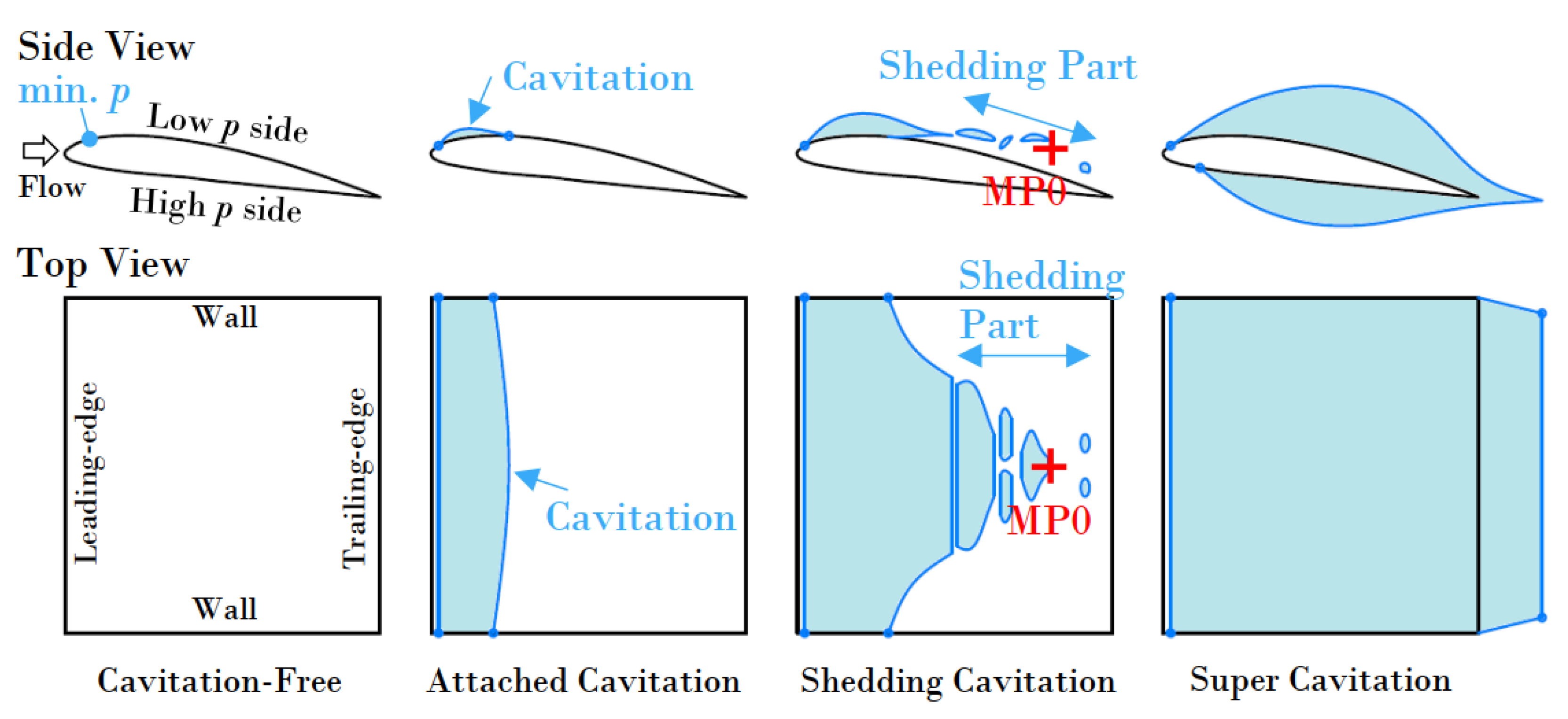
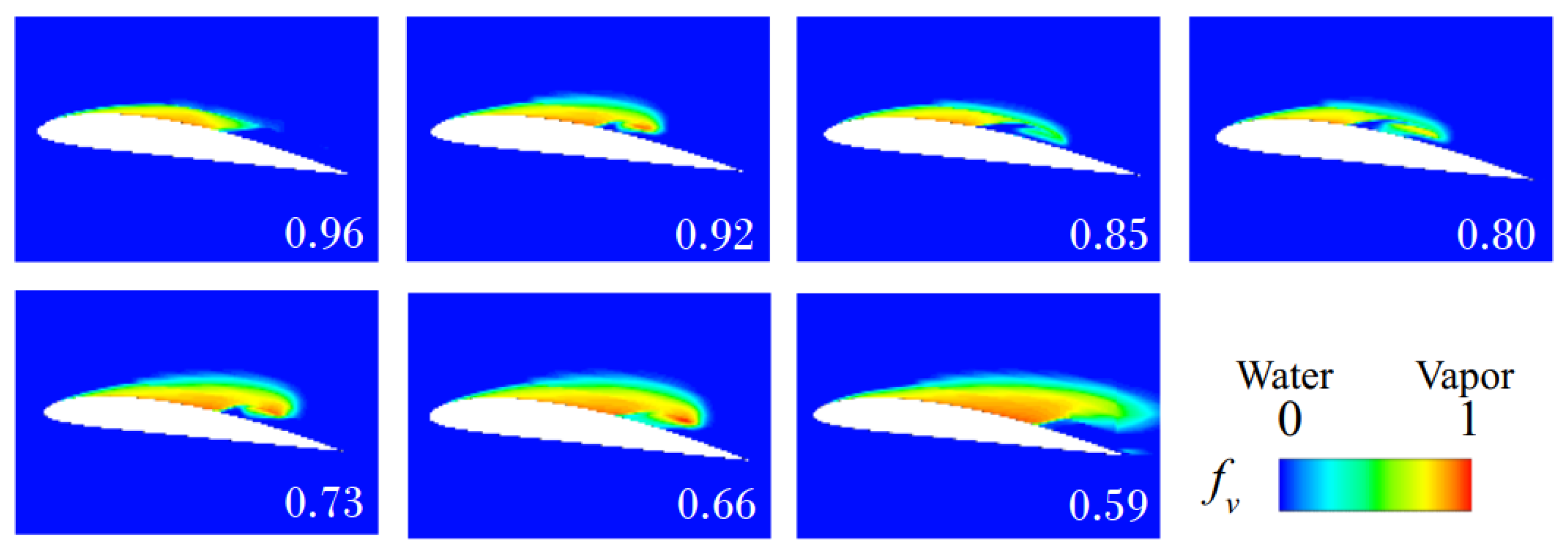
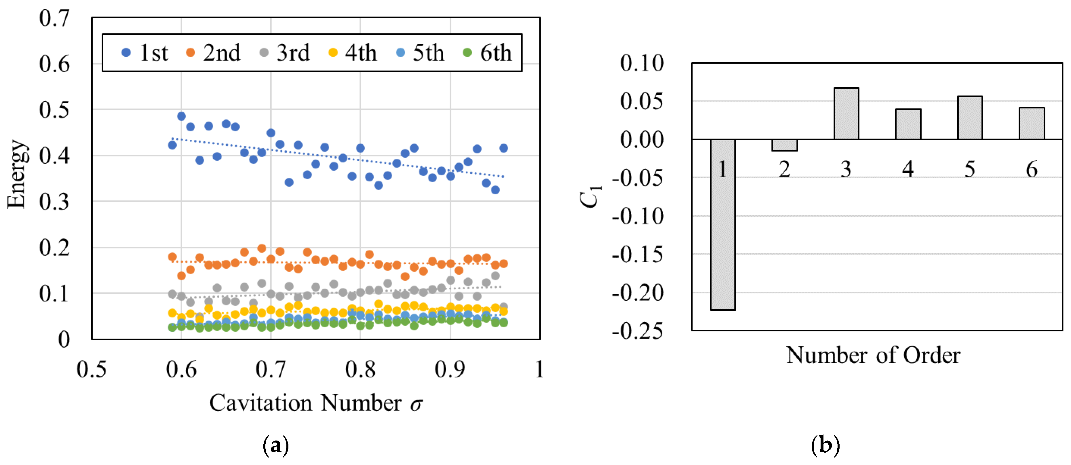
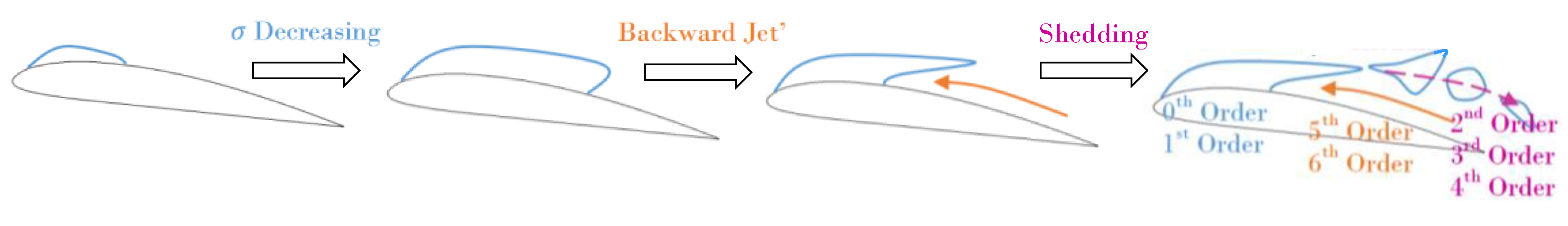
CFD simulation proved effective in predicting the flow field around the hydrofoil. After comparison with the tested data, the capture of velocity fields at different positions was found to be more accurate. The analysis of cavitation two-phase flow using CFD revealed that the size of the cavity varied with the cavitation number σ. As σ decreased from 0.96 to 0.59, the relative length of the cavity increased from 70% of the hydrofoil length to approximately 100%. Additionally, the attached cavity gradually exhibited a downstream shedding phenomenon, forming a shedding cavitation situation.
(b)
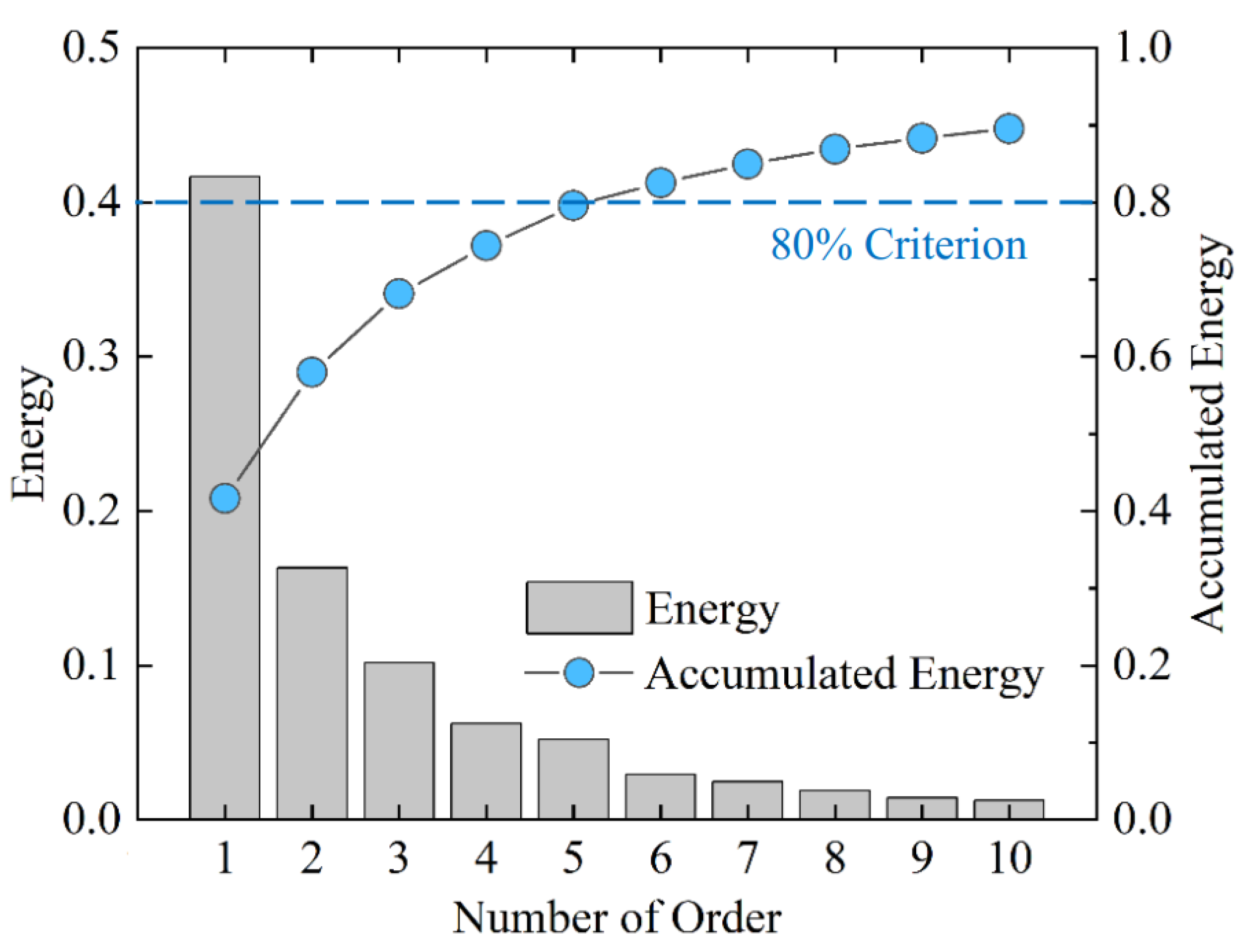
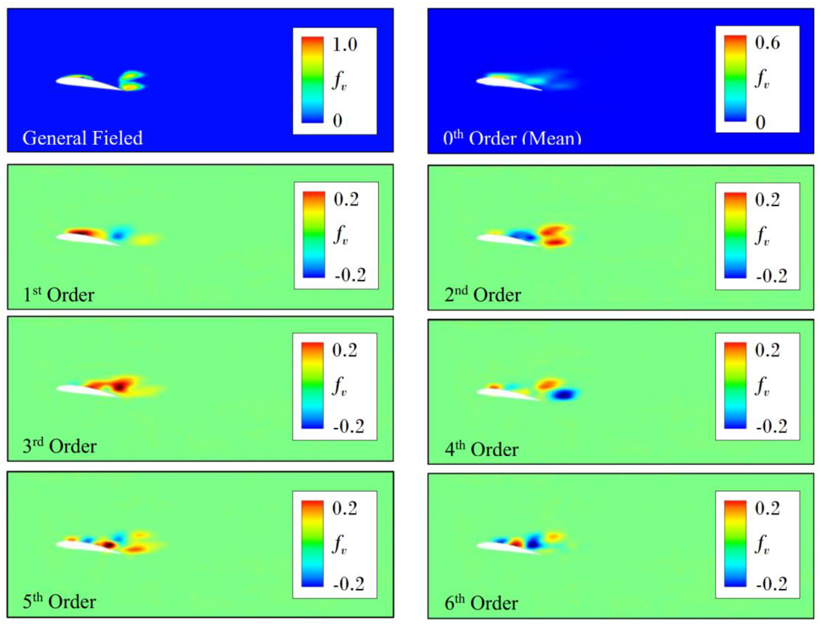
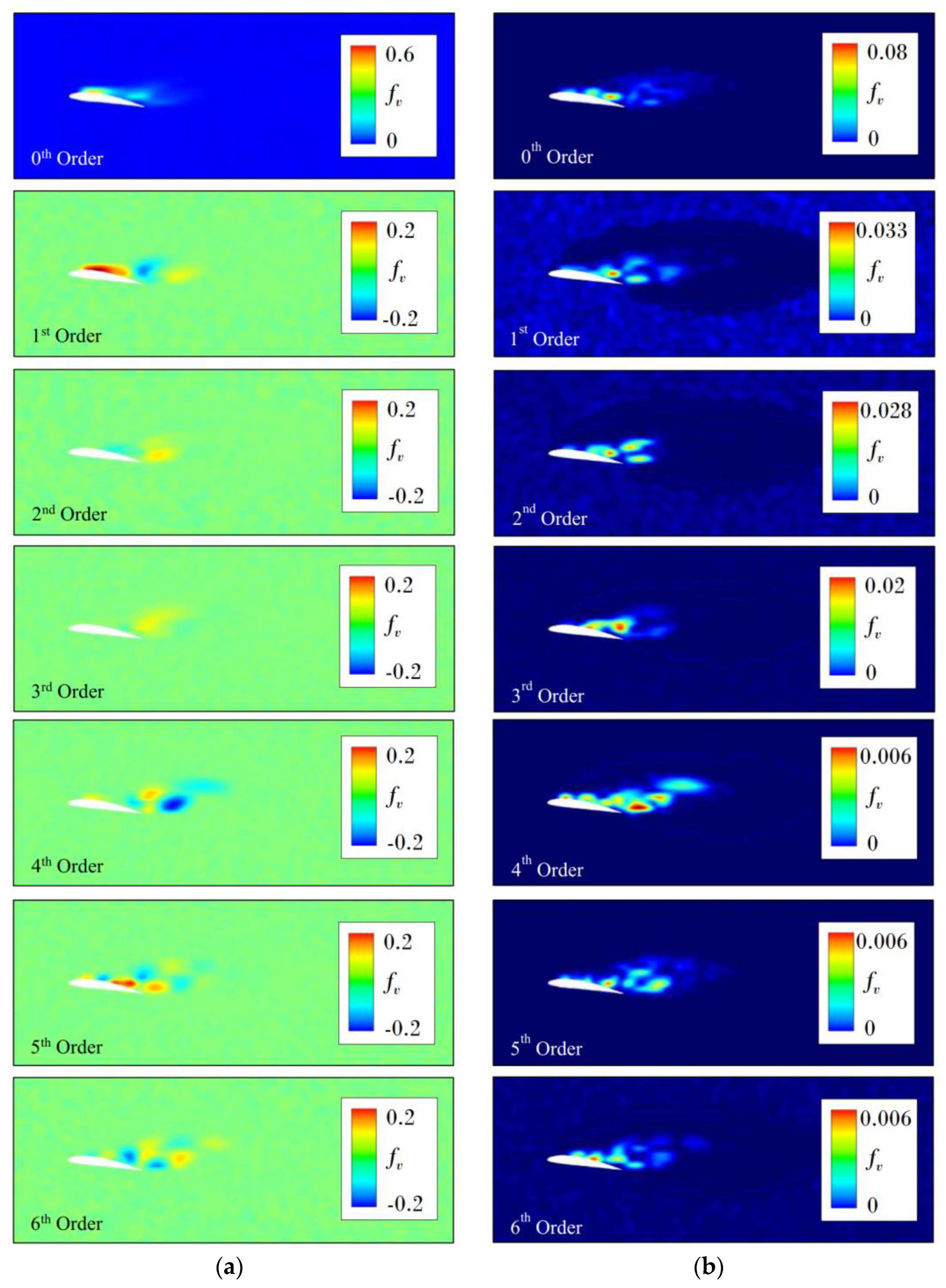
The use of POD enabled effective mode decomposition of the cavitation volume fraction field. Except for the zeroth-order (mean) field, the remaining modes were sorted based on their energy intensity. For instance, taking σ = 0.8 as an example, the 1st order mode energy accounted for over 40%, and the sum of the energies for the first six modes exceeded 80%. The analysis of the corresponding flow phenomenon indicated that the 0th and 1st modes are related to the attachment of a stable cavity, while the 2nd, 3rd, and 4th modes are related to the shedding of cavitation. The 5th and 6th modes along the hydrofoil surface may also be related to the backward jet flow.
(c)
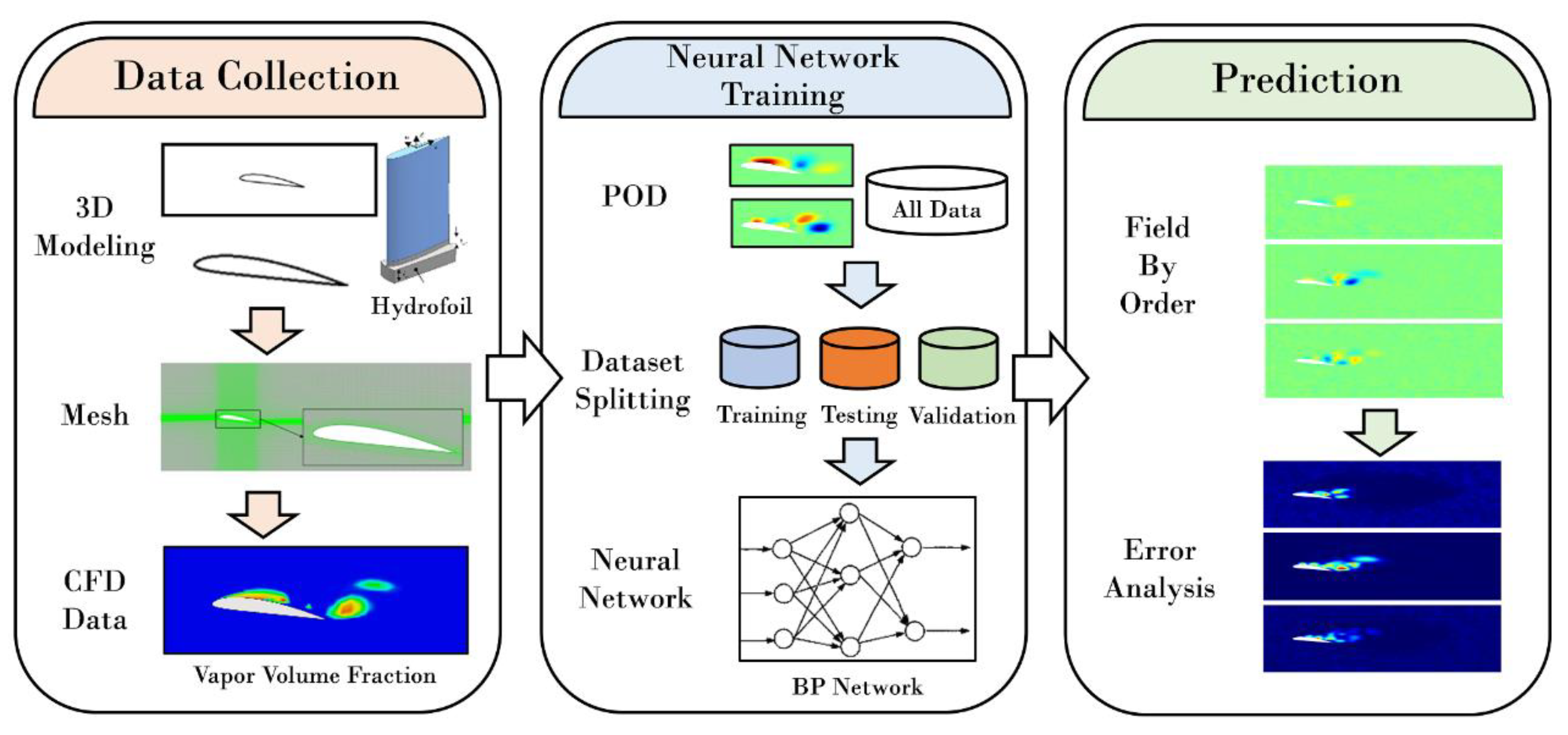
The BP neural network was trained using modal data of CFD-POD under different cavitation numbers. Using the cavitation number σ as input and a vapor volume of 6000 points as output, the cavitation distribution pattern at a certain cavitation number can be predicted. For instance, taking σ = 0.8 as an example, the prediction results of the zeroth- and first-order modes were accurate with minimal errors. However, the prediction of intensity for the third- and fourth-order modes was not as precise, as their contours appeared similar. The prediction effect of the 5th mode was accurate, while the 6th mode showed a slightly worse pattern. For stable cavitation, the neural network performed excellently, but for shedding cavitation, the accuracy of the neural network surrogate model needs further improvement.
In summary, with the increasing complexity of high-dimensional flow fields, the volume of flow field monitoring data will also significantly increase, posing substantial challenges for machine learning and cavitation flow prediction in the research process. Certain aspects of this study may provide reference for related issues in fluid research. Additionally, how to further improve the accuracy of extracting coherent structures in cavitation flow fields and enhance the prediction accuracy and quality of cavitation flow fields will need continuous attention in future research.

Author Contributions

Conceptualization, R.T.; methodology, R.T.; software, P.W.; validation, W.G. and J.Z.; formal analysis, W.G.; investigation, W.G. and Y.W.; resources, P.W., J.Z. and G.F.; data curation, W.G. and L.Y.; writing—original draft preparation, W.G., P.W. and R.T.; writing—review and editing, W.G.; supervision, R.T.; project administration, P.W.; funding acquisition, G.F. All authors have read and agreed to the published version of the manuscript.

Funding

This study was supported by the State Grid Corporation of China Headquarters Technology Project (No. 5400-202324196A-1-1-ZN).

Data Availability Statement

Data are contained within the article.

Conflicts of Interest

The authors declare that they have no conflicts of interest to report regarding the present study. Author Peng Wang, Jinshuai Zhang and Guang Feng was employed by the company State grid Henan Electric Power Research Institute. The remaining authors declare that the research was conducted in the absence of any commercial or financial relationships.

References

  1. Brennen, C.E. Fundamentals of Multiphase Flow; Cambridge University Press: Cambridge, UK, 2005; Available online: https://www.cambridge.org/core/books/fundamentals-of-multiphase-flow/FC7E6D7E54AC9D1C178EDF88D6A75FFF (accessed on 9 January 2024).
  2. Arndt, R.E.A. Cavitation in vortical flows. Annu. Rev. Fluid Mech. 2002, 34, 143–175. [Google Scholar] [CrossRef]
  3. Gogate, P.R.; Kabadi, A.M. A review of applications of cavitation in biochemical engineering/biotechnology. Biochem. Eng. J. 2009, 44, 60–72. [Google Scholar] [CrossRef]
  4. Prosperetti, A. Vapor Bubbles. Annu. Rev. Fluid Mech. 2017, 49, 221–248. [Google Scholar] [CrossRef]
  5. Luo, X.W.; Ji, B.; Tsujimoto, Y. A review of cavitation in hydraulic machinery. J. Hydrodyn. 2016, 28, 35–358. [Google Scholar] [CrossRef]
  6. Ashokkumar, M. The characterization of acoustic cavitation bubbles—An overview. Ultrason. Sonochem. 2011, 18, 864–872. [Google Scholar] [CrossRef] [PubMed]
  7. Petkovsek, R.; Gregorcic, P. A laser probe measurement of cavitation bubble dynamics improved by shock wave detection and compared to shadow photography. J. Appl. Phys. 2007, 102, 391. [Google Scholar] [CrossRef]
  8. Chen, H.S.; Jiang, L.; Chen, D.R.; Wang, J.D. Damages on steel surface at the incubation stage of the vibration cavitation erosion in water. Wear 2008, 265, 692–698. [Google Scholar]
  9. Zhang, X.B.; Qiu, L.M.; Qi, H.; Zhang, X.J.; Gan, Z.H. Modeling liquid hydrogen cavitating flow with the full cavitation model. Int. J. Hydrogen Energy 2008, 33, 7197–7206. [Google Scholar] [CrossRef]
  10. Zhao, W.G.; Zhang, L.X.; Xin, X.P.; Shao, X.M.; Li, W. Numerical simulation of cavitation flow on horizontal axis marine current turbine. J. Mech. Eng. 2011, 47, 171. [Google Scholar] [CrossRef]
  11. Arndt, R.E.A. Cavitation in fluid machinery and hydraulic structures. Annu. Rev. Fluid Mech. 2003, 13, 273–326. [Google Scholar] [CrossRef]
  12. Yonezawa, K.; Konishi, D.; Miyagawa, K. Cavitation surge in a small model test facility simulating a hydraulic power plant. Int. J. Fluid Mach. Syst. 2012, 5, 152–160. [Google Scholar] [CrossRef]
  13. Lee, J.H.; Park, H.G.; Kim, J.H.; Lee, K.J.; Seo, J.S. Reduction of propeller cavitation induced hull exciting pressure by a reflected wave from air-bubble layer. Ocean Eng. 2014, 77, 23–32. [Google Scholar] [CrossRef]
  14. Dular, M.; Bachert, B.; Stoffel, B.; Sirok, B. Relationship between cavitation structures and cavitation damage. Wear 2004, 257, 1176–1184. [Google Scholar] [CrossRef]
  15. Tao, R.; Zhou, X.Z.; Xu, B.C.; Wang, Z.W. Numerical investigation of the flow regime and cavitation in the vanes of reversible pump-turbine during pump mode’s starting up. Renew. Energy 2019, 141, 9–19. [Google Scholar] [CrossRef]
  16. Arabnejad, M.H.; Amini, A.; Farhat, M.; Bensow, R.E. Hydrodynamic mechanisms of aggressive collapse events in leading edge cavitation. J. Hydrodyn. 2020, 32, 6–19. [Google Scholar] [CrossRef]
  17. Escaler, X.; Farhat, M.; Avellan, F.; Egusquiza, E. Cavitation erosion tests on a 2D hydrofoil using surface-mounted obstacles. Wear 2003, 254, 441–449. [Google Scholar] [CrossRef]
  18. Paik, B.G.; Jin, K.; Park, Y.H.; Kim, K.S.; Yu, K.K. Analysis of wake behind a rotating propeller using PIV technique in a cavitation tunnel. Ocean Eng. 2007, 34, 594–604. [Google Scholar] [CrossRef]
  19. Gopalan, S.; Katz, J. Flow structure and modeling issues in the closure region of attached cavitation. Phys. Fluids 2000, 12, 895–911. [Google Scholar] [CrossRef]
  20. Barre, S.; Rolland, J.; Boitel, G.; Goncalves, E. Experiments and modeling of cavitating flows in Venturi: Attached sheet cavitation. Eur. J. Mech. B/Fluids 2009, 28, 444–464. [Google Scholar] [CrossRef]
  21. Shi, S.; Wang, G.; Wang, F.; Gao, D. Experimental study on unsteady cavitation flows around three-dimensional hydrofoil. Chin. J. Appl. Mech. 2011, 28, 105–110. [Google Scholar]
  22. Melissaris, T.; Bulten, N.; Terwisga, T.J.C. On the applicability of cavitation erosion risk models with a URANS solver. J. Fluids Eng. 2019, 141, 1011104. [Google Scholar] [CrossRef]
  23. Luo, H.; Tao, R. Prediction of the cavitation over a twisted hydrofoil considering the nuclei fraction sensitivity at 4000m altitude level. Water 2021, 13, 1938. [Google Scholar] [CrossRef]
  24. Ravelet, F.; Danlos, A.; Bakir, F.; Croci, K.; Khelladi, S. Development of attached cavitation at very low Reynolds numbers from partial to super-cavitation. Appl. Sci. 2020, 10, 7350. [Google Scholar] [CrossRef]
  25. Dreyer, M.; Decaix, J.; Münch-Alligné, C.; Farhat, M. Mind the gap: A new insight into the tip leakage vortex using stereo-PIV. Exp. Fluids 2014, 55, 1849. [Google Scholar] [CrossRef]
  26. Hu, Z.L.; Wu, Y.Z.; Li, P.X.; Xiao, R.F.; Tao, R. Comparative study on the fractal and fractal dimension of the vortex structure of hydrofoil’s tip leakage flow. Fractal Fract. 2023, 7, 123. [Google Scholar] [CrossRef]
  27. Liu, J.B.; Bao, Y.; Zheng, W.T. Analyses of some structural properties on a class of hierarchical scale-free networks. Fractals 2022, 30, 2250136. [Google Scholar] [CrossRef]
  28. Liu, J.B.; Bao, Y.; Zheng, W.T.; Hayat, S. Network coherence analysis on a family of nested weighted n-polygon networks. Fractals 2022, 29, 2150260. [Google Scholar] [CrossRef]
  29. Franc, J.P.; Miche, J.M. Fundamentals of Cavitation; Kluwer Academic Publishers: Amsterdam, The Netherlands, 2004; Available online: https://link.springer.com/book/10.1007/1-4020-2233-6 (accessed on 9 January 2024).
  30. Tao, T. A quantitative formulation of the global regularity problem for the periodic Navier-Stokes equation. Dyn. Partial Differ. Equ. 2007, 4, 293–302. [Google Scholar] [CrossRef]
  31. Březina, J. Asymptotic behavior of solutions to the compressible Navier-Stokes equation around a time-periodic parallel flow. SIAM J. Math. Anal. 2013, 45, 3514–3574. [Google Scholar] [CrossRef]
  32. Pitsch, H. Large-Eddy simulation of turbulent combustion. Annu. Rev. Fluid Mech. 2006, 38, 453–482. [Google Scholar] [CrossRef]
  33. Spalart, P.R. Detached-Eddy Simulation. Annu. Rev. Fluid Mech. 2009, 41, 181–202. [Google Scholar] [CrossRef]
  34. Zhong, X.; Wang, X. Direct numerical simulation on the receptivity, Instability, and transition of hypersonic boundary layers. Annu. Rev. Fluid Mech. 2012, 44, 527–561. [Google Scholar] [CrossRef]
  35. Menter, F.R.; Kuntz, M.; Langtry, R. Ten years of industrial experience with the SST turbulence model. Turbul. Heat Mass Transf. 2003, 4, 625–632. [Google Scholar]
  36. Vinuesa, R.; Steven, L.B. Enhancing computational fuid dynamics with machine learning. Nat. Comput. Sci. 2022, 2, 358–366. [Google Scholar] [CrossRef] [PubMed]
  37. Díez, P.; Muíxí, A.; Zlotnik, S. Nonlinear dimensionality reduction for parametric problems: A kernel Proper Orthogonal Decomposition (kPOD). Int. J. Numer. Methods Eng. 2021, 122, 7306–7327. [Google Scholar] [CrossRef]
  38. Kaheman, K.; Brunto, S.L.; Kutz, J.N. Automatic differentiation to simultaneously identify nonlinear dynamics and extract noise probability distributions from data. Mach. Learn. Sci. Technol. 2022, 3, 015031. [Google Scholar] [CrossRef]
  39. Brunton, S.; Noack, B.R.; Koumoutsakos, P. Machine learning for fluid mechanics. Annu. Rev. Fluid Mech. 2020, 52, 477–508. [Google Scholar] [CrossRef]
  40. Kou, J.; Zhang, W. An approach to enhance the generalization capability of nonlinear aerodynamic reduced-order models. Aerosp. Sci. Technol. 2016, 49, 197–208. [Google Scholar] [CrossRef]
  41. Jin, F.Y.; Tao, R.; Lu, Z.H.; Xiao, R.F. A spatially distributed network for tracking the pulsation signal of flow field based on CFD simulation: Method and a case study. Fractal Fract. 2021, 5, 181. [Google Scholar] [CrossRef]
  42. Charkrit, S.; Shrestha, P.; Liu, C.Q. Liutex core line and POD analysis on hairpin vortex formation in natural flow transition. J. Hydrodyn. 2020, 32, 1109–1121. [Google Scholar] [CrossRef]
  43. Schmid, P.J. Dynamic mode decomposition of numerical and experimental data. J. Fluid Mech. 2010, 656, 5–28. [Google Scholar] [CrossRef]
  44. Liberge, E.; Hamdouni, A. Reduced Order Modelling method via Proper Orthogonal Decomposition (POD) for flow around an oscillating cylinder. J. Fluids Struct. 2010, 26, 292–311. [Google Scholar] [CrossRef]
  45. Xie, L.; Jin, S.Y.; Wang, Y.Z.; Yu, J. PIV measurement and POD analysis of inner flow field in 90°bending duct of circular-section with fore-end valve. J. Exp. Fluid Mech. 2012, 26, 21–25. [Google Scholar]
  46. Liu, M.; Tan, L.; Cao, S. Dynamic mode decomposition of cavitating flow around ALE 15 hydrofoil. Renew. Energy 2019, 139, 214–227. [Google Scholar] [CrossRef]
  47. Wu, L.; Chen, K.; Zhan, C. Snapshot POD analysis of transient flow in the pilot stage of a jet pipe servo valve. J. Turbul. 2018, 19, 889–909. [Google Scholar] [CrossRef]
  48. Resseguier, V.; Mémin, E.; Heitz, D.; Chapron, B. Stochastic modelling and diffusion modes for POD models and small-scale flow analysis. J. Fluid Mech. 2017, 826, 888–917. [Google Scholar] [CrossRef]
  49. Wu, Y.Z.; Tao, R.; Yao, Z.F.; Xiao, R.F.; Wang, F.J. Application and comparison of dynamic mode decomposition methods in the tip leakage cavitation of a hydrofoil case. Phys. Fluids 2023, 35, 023326. [Google Scholar] [CrossRef]
  50. Huang, B.; Wang, G.Y.; Zhao, Y.; Wu, Q. Physical and numerical investigation on transient cavitating flows. Sci. China Technol. Sci. 2013, 56, 2207–2218. [Google Scholar] [CrossRef]
  51. Wu, Y.Z.; Li, P.X.; Tao, R.; Zhu, D.; Xiao, R.F. Improvement of mode selection criterion of dynamic mode decomposition in a hydrofoil cavitation multiphase flow case. Ocean Eng. 2022, 265, 112579. [Google Scholar] [CrossRef]
  52. Menter, F.R. Two-equation eddy-viscosity turbulence models for engineering applications. AIAA J. 1994, 32, 1598–1605. [Google Scholar] [CrossRef]
  53. Zwart, P.J.; Gerber, A.G.; Belamri, T. A two-phase flow model for predicting cavitation dynamics. In Proceedings of the Fifth International Conference on Multiphase Flow, Yokohama, Japan, 30 May–4 June 2004. [Google Scholar]
  54. Bao, Y.D.; Wu, Y.P.; He, Y. Optimal mix forecasting method based on BP neural network and its application. J. Agric. Mech. Res. 2004, 3, 162–164. [Google Scholar]
  55. Dular, M.; Bachert, R.; Schaad, C.; Stoffel, B. Investigation of a re-entrant jet reflection at an inclined cavity closure line. Eur. J. Mech. B/Fluids 2007, 26, 688–705. [Google Scholar] [CrossRef]
  56. Trummler, T.; Schmidt, S.J.; Adams, N.A. Investigation of condensation shocks and re-entrant jet dynamics in a cavitating nozzle flow by Large-Eddy Simulation. Int. J. Multiph. Flow 2020, 125, 103215. [Google Scholar] [CrossRef]
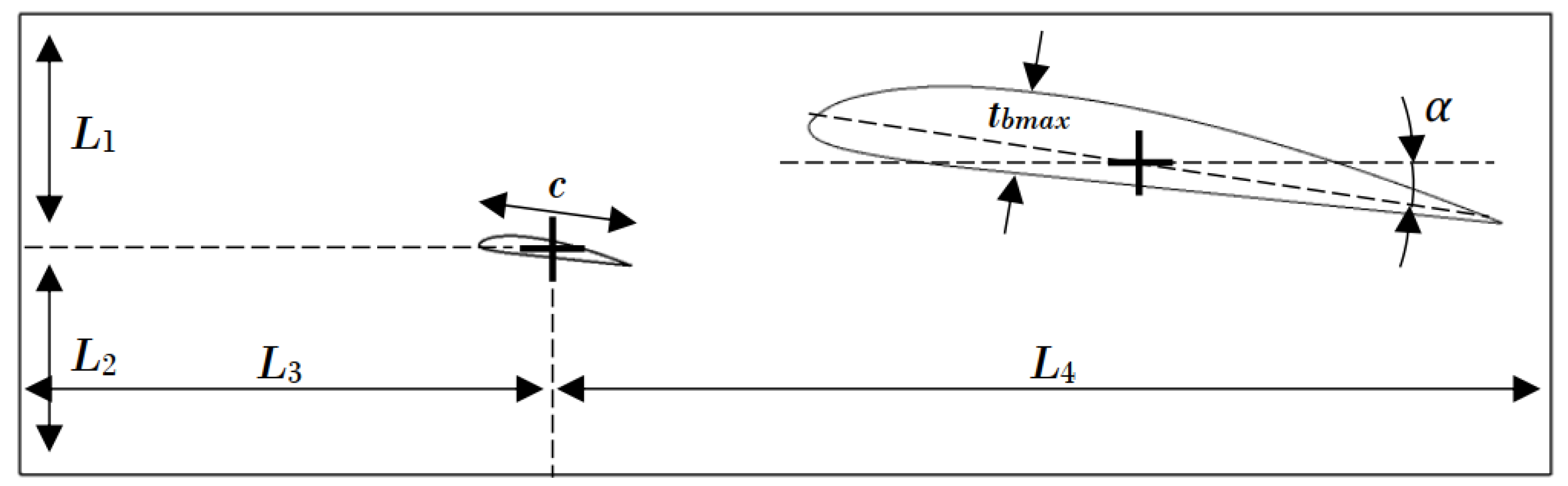
Figure 1. Cavitation process on the phase diagram.
Jmse 12 00148 g001
Figure 2. Schematic map of cavitation over hydrofoil.
Jmse 12 00148 g002
Figure 3. Schematic map of pressure pulsation in cavitation-free status and vapor volume fraction pulsation in shedding cavitation status.
Jmse 12 00148 g003
Figure 4. Computational domain of Clark-Y hydrofoil’s cavitation.
Jmse 12 00148 g004
Figure 5. Computational domain with boundary conditions.
Jmse 12 00148 g005
Figure 6. Mesh of fluid domain for CFD simulation.
Jmse 12 00148 g006
Figure 7. Comparison of velocity distribution between CFD and tested data at σ = 0.8 [49].
Jmse 12 00148 g007
Figure 8. Cavitation vapor volume distribution at different cavitation numbers.
Jmse 12 00148 g008
Figure 9. Energy of modes by order at σ = 0.8.
Jmse 12 00148 g009
Figure 10. Volume fraction distribution and its different order modes at a time step of cavitation shedding at σ = 0.8.
Jmse 12 00148 g010
Figure 11. Energy law of modes. (a) Mode’s energy variation with cavitation number; (b) law of the first-order term in linear fitting.
Jmse 12 00148 g011
Figure 12. Workflow of the neural network-based study.
Jmse 12 00148 g012
Figure 13. Neural network predicted cavitation volume fraction distribution by POD modes at a time step of cavitation shedding at σ = 0.8. (a) Neural network predicted value; (b) error against CFD-POD data.
Jmse 12 00148 g013
Figure 14. Discussion on the relationship between cavitating flow posture (mode) and flow phenomena.
Jmse 12 00148 g014
Table 1. Parameters of the Clark-Y hydrofoil cavitation case.
ParameterValueUnitDescription
L1105mm1.5 c length
L2105mm1.5 c length
L3245mm3.5 c length
L4455mm6.5 c length
c70mmchord
tbmax8.27mmmaximum thickness
α8degreesincidence angle
Disclaimer/Publisher’s Note: The statements, opinions and data contained in all publications are solely those of the individual author(s) and contributor(s) and not of MDPI and/or the editor(s). MDPI and/or the editor(s) disclaim responsibility for any injury to people or property resulting from any ideas, methods, instructions or products referred to in the content.

