Analysis of Stress–Strain Characteristics and Signal Coherence of Low-Specific-Speed Impeller Based on Fluid–Structure Interaction

Abstract

In this study, an analysis of a low-specific-speed pump is carried out based on the methods of one-way and two-way fluid–structure interactions (FSIs). This study analyzes the influence of FSIs on the internal flow field and external characteristics of the pump. Utilizing a two-way FSI, the signal coherence analysis method is employed to analyze the coherence of signals between the flow field and the structural field. Addressing the issue of a lack of a connection between the two signals, this study bridges a gap in the existing research. The results indicate that different interaction methods have certain influences on impeller stress and deformation. However, in both coupling modes, the maximum deformation and the maximum equivalent stress have the same distribution position. The head error obtained using the two-way coupling method is lower than that of the uncoupled results, which indicates that the two-way FSI calculation results are closer to the experimental results. The pressure pulsation signals at the interface of the impeller and volute exhibit strong coherence with the structural field signals. For low-specific-speed centrifugal pumps, establishing a clear connection between the flow field signals and structural field signals will help guide further optimization of their performance through design.

1. Introduction

As a common basic pump type, centrifugal pumps are widely used in the petrochemical industry, the aerospace industry, ocean engineering, hydraulic engineering, agricultural production, and other fields [1,2,3]. In industrial applications, centrifugal pumps with specific speed values between 50 and 80 are often specified as low-specific-speed centrifugal pumps [4,5,6]. Low-specific-speed centrifugal pumps, as members of the centrifugal pump family, possess a unique application value in the industrial field. Their low-speed design allows them to perform exceptionally well in scenarios involving high-viscosity liquids and media containing particulate matter and in applications requiring significant head. A low-specific-speed centrifugal pump has the characteristics of a low flow rate, high head, and a compact structure [7,8]. Compared to high-speed centrifugal pumps, low-speed centrifugal pumps are more suitable for the transportation of certain special media. Their lower speed helps reduce friction losses between the pump and the medium, thereby improving pump efficiency. Simultaneously, low-specific-speed centrifugal pumps typically have larger impeller diameters. This design ensures a sufficient flow rate and sufficient head at low speeds. However, it may also increase the inertial torque of the impeller, making it more prone to vibrations during rotation [9]. Compared to closed impellers, semi-open impellers are easy to clean and are less prone to clogging. However, their structures are more brittle. For a semi-open impeller, compared with a closed impeller, the stress is relatively small and the manufacturing process is simple. A semi-open impeller is generally used to transport liquids that easily precipitate or those containing granular media [10,11]. When the natural frequency of the pump is the same as the hydraulic excitation frequency, resonance will occur, which can affect the safety and stability of pump operation [12,13]. The rotating components of a low-specific-speed centrifugal pump, especially the impeller and shaft, may have lower natural frequencies due to their larger sizes and masses. During operation, if external excitation frequencies are close to or match these natural frequencies, it can easily lead to resonance and vibration, potentially causing structural damage and a decline in the performance of the centrifugal pump. Hence, it is particularly important to analyze the internal stress–strain characteristics and modal mechanical characteristics of low-specific-speed centrifugal pumps [14,15]. However, for the unsteady and complex flow in a pump, the pressure distribution on the impeller is uneven, which results in slight deformation. Meanwhile, the deformation of the impeller will also affect the flow field structure in the pump [16,17]. In order to understand the mutual coupling relationship between the flow field and the structural field, it is necessary to consider the numerical simulation analysis of the internal flow field of the centrifugal pump with low specific speed under the action of the FSI. In addition, due to the limitations of the installation positions of experimental strain gauges and the large error in the measurement of small stresses and strains, the FSI stress–strain analysis based on numerical simulation has become an effective method to predict the deformation and noise of the pump body [18,19]. Afra et al. [20] proposed a hybrid model that includes an explicit Lattice Spring Model and an Immersed Boundary non-Newtonian Lattice Boltzmann Method to simulate the behavior of a filament in the vicinity of a fluid flow. That study provides a methodological reference for the present work. Delouei et al. [21] used similar methods to investigate the falling manners of non-circular particles in an enclosure while the pulsatile flow was involved as a counter-flow, and the accuracy of the results was well demonstrated. Jiang et al. [22] used the method of sequential coupling to find that the unsteady flow of the fluid in a pump is the main reason for the vibration and noise of the pump. Li et al. [23] used the FSI method to study the vibration characteristics of the impeller of a large mixed-flow pump during the start-up process. They found that frequent starts had a detrimental effect on the edge of the impeller, resulting in severe deformation of the blade tip and affecting the normal operation of the pump. However, they did not consider the signal correlation between the structural field and the flow field. Kato et al. [24] calculated the pressure pulsation on the inner surface of a five-stage centrifugal pump by combining flow and structural analyses, and they used the one-way FSI method to predict the noise on the outer surface of the centrifugal pump. The results show that this method can effectively reduce the flow-induced noise generated by hydraulic impeller machinery. Macphee et al. [25] designed deformable blades by combining experiments with FSI simulations, thereby improving the efficiency of axial wind turbines. Benra et al. [26] also considered the effect of a fluid on a solid and the reaction of a solid on a fluid. They conducted a coupled analysis of a pump rotor and a flow field and compared it with an experiment, but the research object was limited to a single-blade non-clogging centrifugal pump. Meanwhile, a two-way FSI can result in unstable coupling between a flow field and a solid field and is often associated with added mass effects. Degroote [27] conducted a meticulous study on this issue, placing a particular emphasis on researching partitioned simulation techniques for strongly coupled FSI problems. In summary, researchers have conducted numerous studies on the internal flow and structural performance of pumps. However, they have not adequately considered the impact of structural deformations on flow field calculations. Additionally, there is a lack of research regarding the coherence between pressure pulsation signals within the flow field and signals from the structural field. This study primarily focuses on the stress–strain characteristics of low-speed centrifugal pumps, as well as the coherence between flow field signals and structural field signals. Through these investigations, the aim is to gain a deeper understanding of the performance and operational mechanisms of low-speed centrifugal pumps. The adoption of one-way and two-way FSI methods can provide a more comprehensive analysis, taking into account the complexity of the interaction between the fluid and the structure. This study contributes an in-depth numerical analysis to the field of low-specific-speed centrifugal pumps, revealing stress–strain characteristics and the interrelationship between flow field and structural field signals. This not only aids in optimizing pump design and performance but also provides valuable insights for engineering practices in similar systems.

In this study, based on the computer fluid dynamics (CFD) numerical simulation method, a four-blade low-specific-speed centrifugal pump is the research object, and the stress–strain simulation results and modal simulation results are compared and analyzed under the consideration of the two methods of one-way and two-way FSIs. Numerical simulation analysis is of great significance for gaining a deep understanding of and optimizing system behavior, reducing research costs, improving research efficiency, and addressing experimental challenges. Simultaneously, utilizing a two-way FSI, the signal coherence analysis method is used to analyze the signal coherence between the pressure pulsation signal of the flow field and the maximum deformation and maximum equivalent stress of the structural field. This study can provide effective guidance for solving the vibration problem and the fault diagnosis of low-specific-speed centrifugal pumps.

2. Numeral Calculations

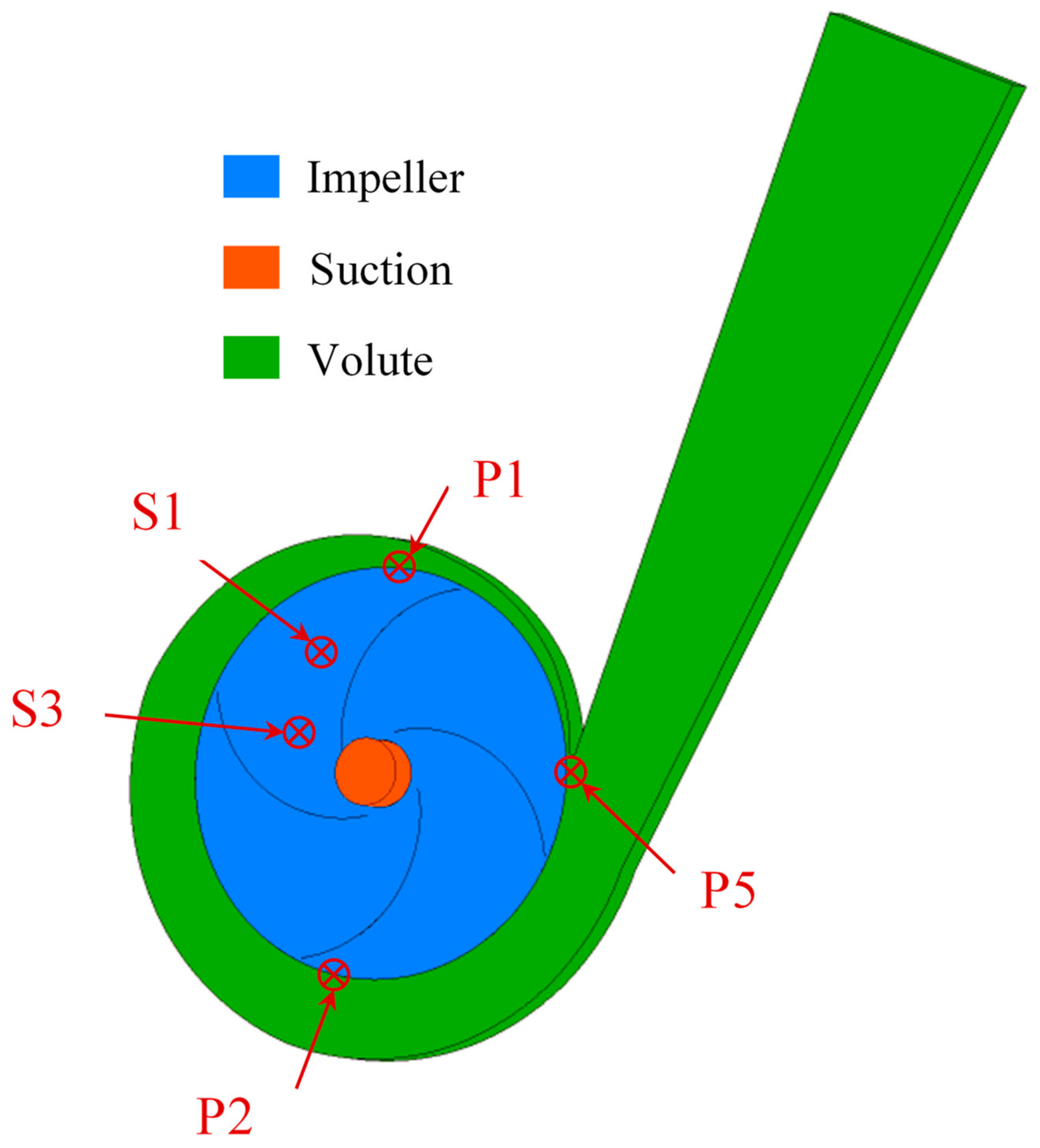
2.1. Objective Pump Model

The research object of this study is a semi-open low-specific-speed centrifugal pump used in the experiments of Choi et al. [5]. The computational domain of the flow field consists of three parts: the section, the impeller, and the volute. This structure is shown in Figure 1. In order to accurately monitor the pressure pulsation signals generated at different locations within the fluid domain of the centrifugal pump, we positioned pressure pulsation monitoring points at representative locations. At the interface between the impeller and the volute, we placed two monitoring points, denoted as P1 and P3, which were located at positions corresponding to 90° and 270° of impeller rotation, respectively. Additionally, we installed a monitoring point, labeled P5, at the cut-water of the volute, and two monitoring points were installed within the impeller passageway, marked as S1 and S3.

We observed the detailed characteristics of the internal flow field of the low-specific-speed centrifugal pump using Particle Image Velocimetry (PIV) and found that the internal flow characteristics of the low-specific-speed impeller are complex and that these characteristics are the reason for its unique performance in the low-specific-speed range. The basic design parameters of the pump are shown in

Table 1. Basic structural parameters of the model pump.

Parameter	Numerical Value	Unit
Number of blades (Z)	4	[-]
Specific speed (ns)	60.28	[-]
Design rotation speed (nd)	700	r/min
Design flow rate (Qd)	0.4745	kg/s
Design head (Hd)	0.899	m

.

The specific speed (ns) is defined in Equation (1). It is an integrated characteristic number. Q is the flow rate, H is the head, and n is the rotation speed. It is the basis for calculating pump structure parameters.

$$n_s=\frac{3.65n\sqrt{Q}}{H^{3/4}}$$

(1)

In both the experiment and the numerical simulation, the pump head (H) is calculated using Equation (2), and the efficiency (η) is calculated using Equation (3) given below.

$$H=\frac{P_{out}-P_{in}}{\rho g}$$

(2)

In Equation (2), P_out is the average total pressure at the pump outlet, P_in is the average total pressure at the pump inlet, and g is the acceleration of gravity.

$$\eta =\frac{\rho gQH}{M{\omega }_0}$$

(3)

In Equation (3), M is the impeller torque and ω₀ is the impeller angular velocity.

2.2. Objective Pump Model

In order to obtain the flow characteristics in the flow field before the FSI and the pressure load on the FSI surface, it is necessary to perform unsteady calculations on the flow field in the computational domain. The impeller is the rotation domain, and the rest of the structure is the stationary domain. Taking the steady-state calculation result as the initial condition, the inlet is set as the pressure boundary, and the pressure value is 1 atm. The outlet is set as the flow rate boundary, and flow rate value is 0.4745 kg/s. All the walls are set as non-slip walls. The calculation is performed every two degrees of impeller rotation; that is, each rotation period is divided into 180 time steps. Each time step is 0.000476 s, and the impeller rotates 10 revolutions in total. The convergence criteria of the continuity equation and the momentum equation are both 10⁻⁵. The governing equations are shown below.

The continuity equation is

$$\frac{\partial \rho }{\partial t}+\frac{\partial (\rho v_x)}{\partial x}+\frac{\partial (\rho v_y)}{\partial y}+\frac{\partial (\rho v_z)}{\partial z}=0$$

(4)

where ρ is the density of the fluid medium; t is time; and v_x, v_y, and v_z are the components of the velocity vector in the X, Y, and Z directions, respectively.

The momentum equation is

$$\frac{\partial (\rho v)}{\partial t}+(\rho v\cdot \nabla )v=-\nabla p+\mu {\nabla }^{2}v+\rho f$$

(5)

where μ is the dynamic viscosity coefficient of the fluid, v is the velocity vector, ▽ is the Hamilton operator, and f is the stress vector.

Both the steady and unsteady calculations use the SST (shear stress transport) k-ω turbulence model, which can accurately calculate the complex flow at the rotor–stator interaction and in the near-wall region. It can achieve the transformation between the k-ω model and k-ε and considers the effects of turbulent shear stress transfer in the reverse-pressure boundary layer. The eddy viscosity coefficient is corrected to a certain extent. Therefore, these characteristics make the SST k-ω turbulence model more advantageous for wall treatment and more suitable for the simulation analysis of fluid machinery turbulence [28]. The transformation form of the two models is as follows:

The eddy viscosity limit equation is

$$v=\frac{a_{1}k}{\max \left(a_1\omega ,S{F}_2\right)}$$

(6)

The mixed-function expression is as follows:

$$F_1=\tanh \left(\min {\left(\max \left(\frac{\sqrt{k}}{{\beta }^{*}\omega y},\frac{500v}{y^2\omega }\right),\frac{4\rho k}{C{D}_{k\omega }{\sigma }_{\omega 2}{y}^2}\right)}^4\right)$$

(7)

$$C{D}_{k\omega }=\max \left(2\rho \frac{1}{{\sigma }_{\omega 2}\omega }\frac{\partial k}{\partial x_j}\frac{\partial \omega }{\partial x_j},1.0\times {10}^{-10}\right)$$

(8)

$$F_2=\tanh \left({\left(\max \left(\frac{2\sqrt{k}}{{\beta }^{*}\omega y},\frac{500v}{y^2\omega }\right)\right)}^2\right)$$

(9)

where y is the closest distance to the wall, ν is the kinematic viscosity, k is the turbulent kinetic energy, and ω is the dissipation rate of the specific energy. β* is the empirical coefficient, which usually takes a value of 0.09, σ_ω2 = 0.856. Hence, the SST k-ω turbulence model behaves as a k-ω method near the wall, where F₁ = 1, and at a distance away from the wall, where F₁ = 0, it behaves as a k-ε method.

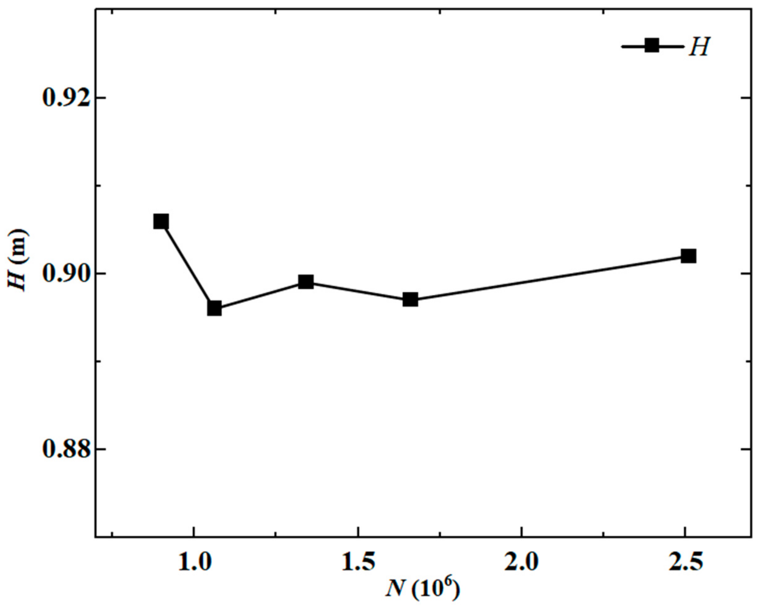
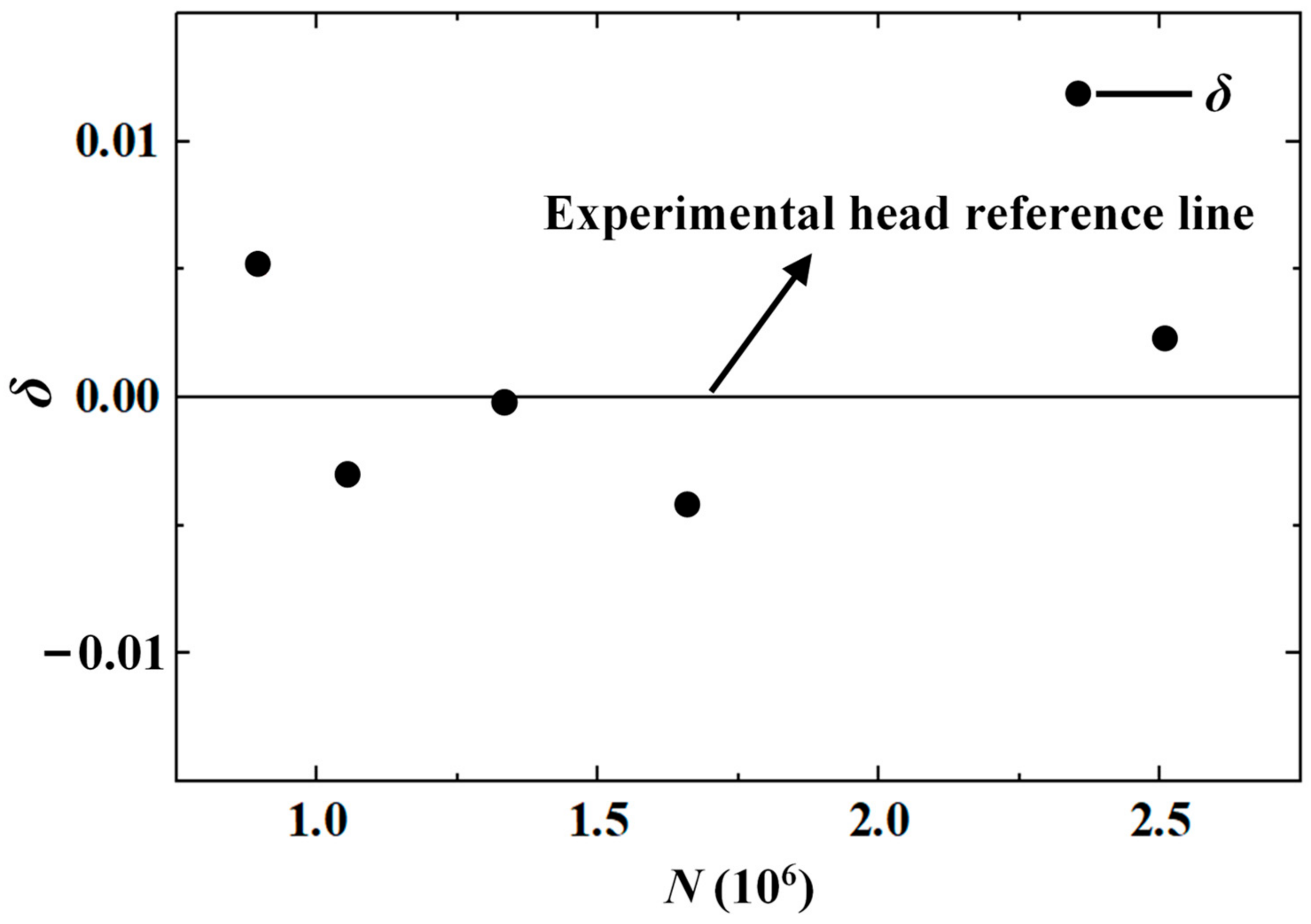
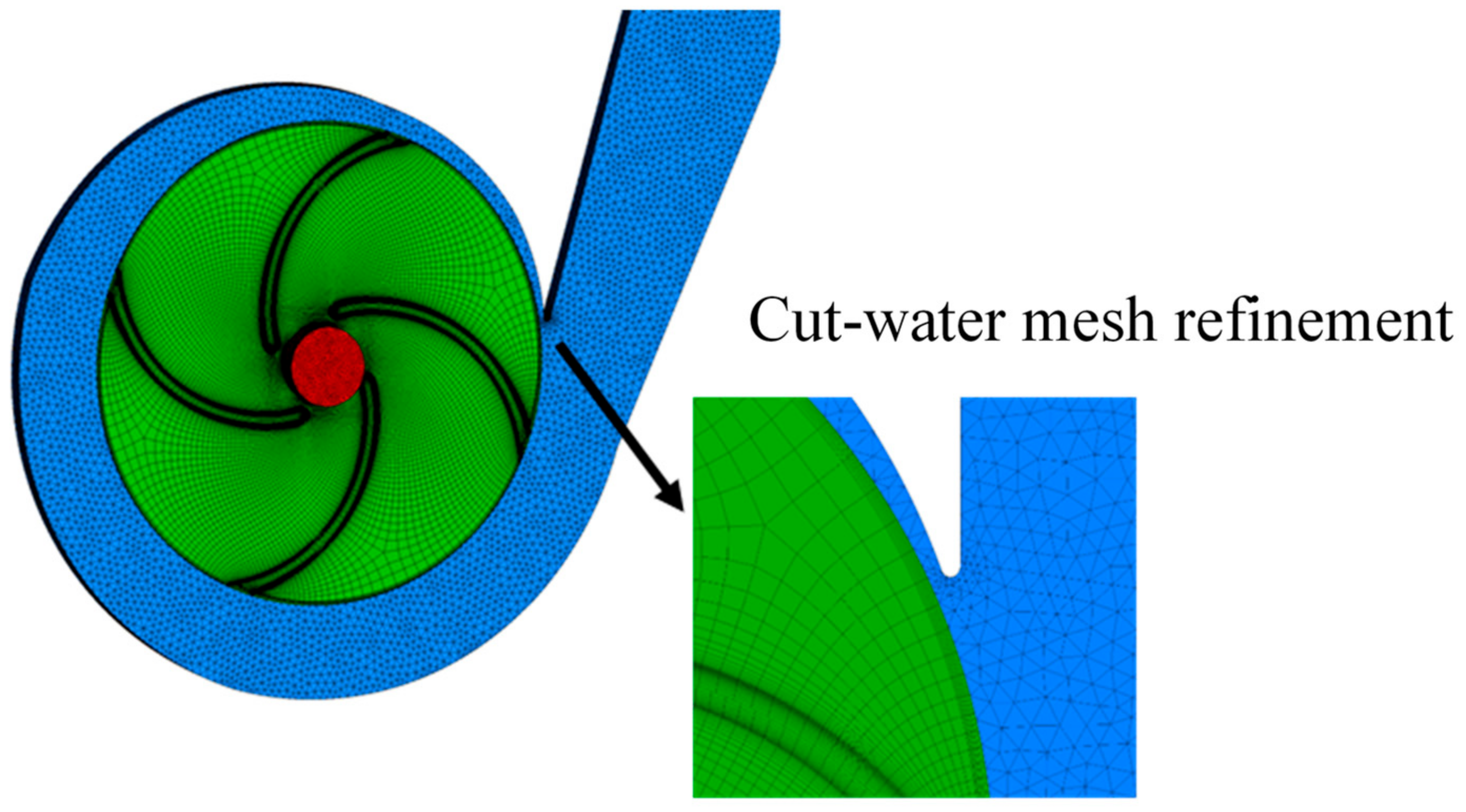
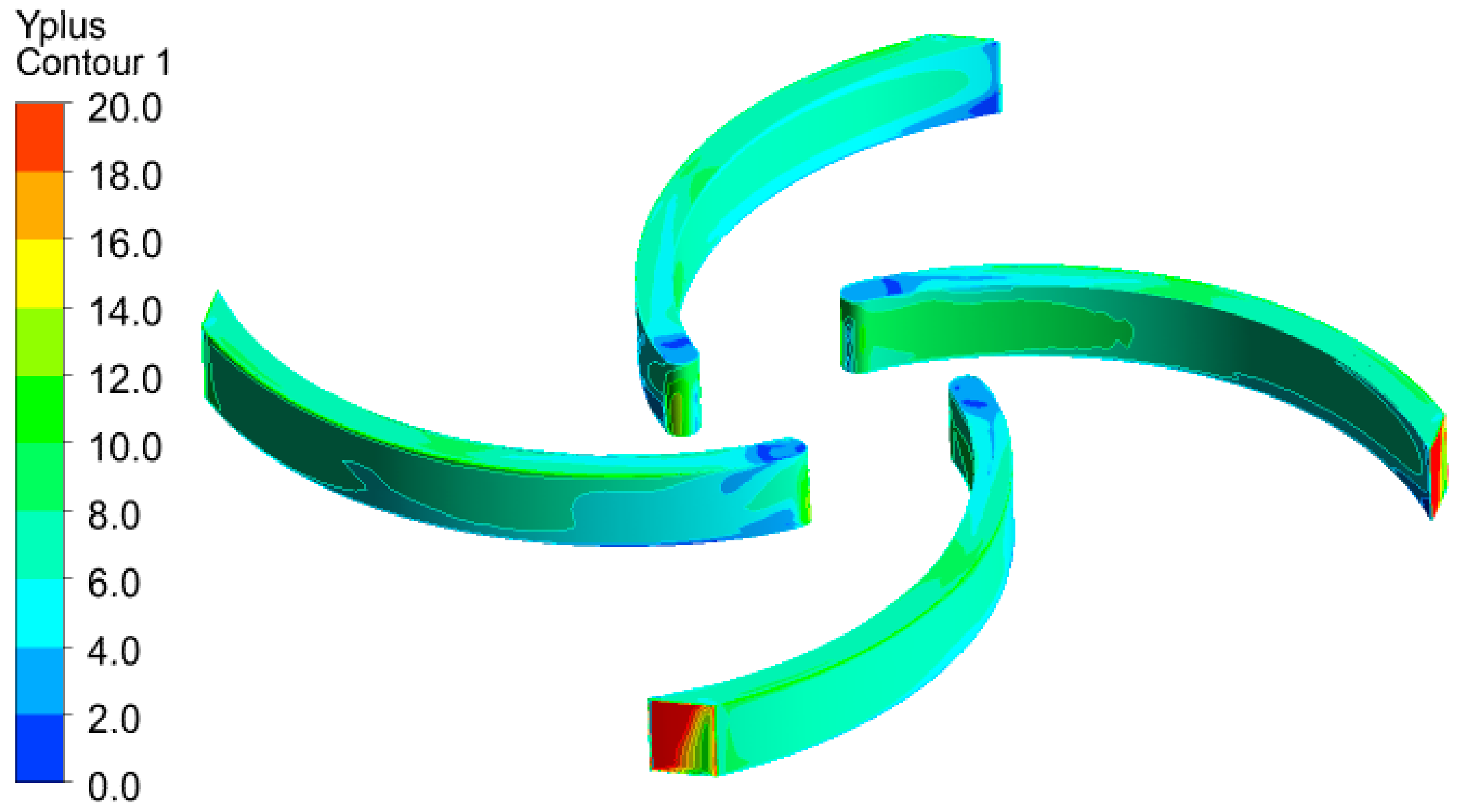
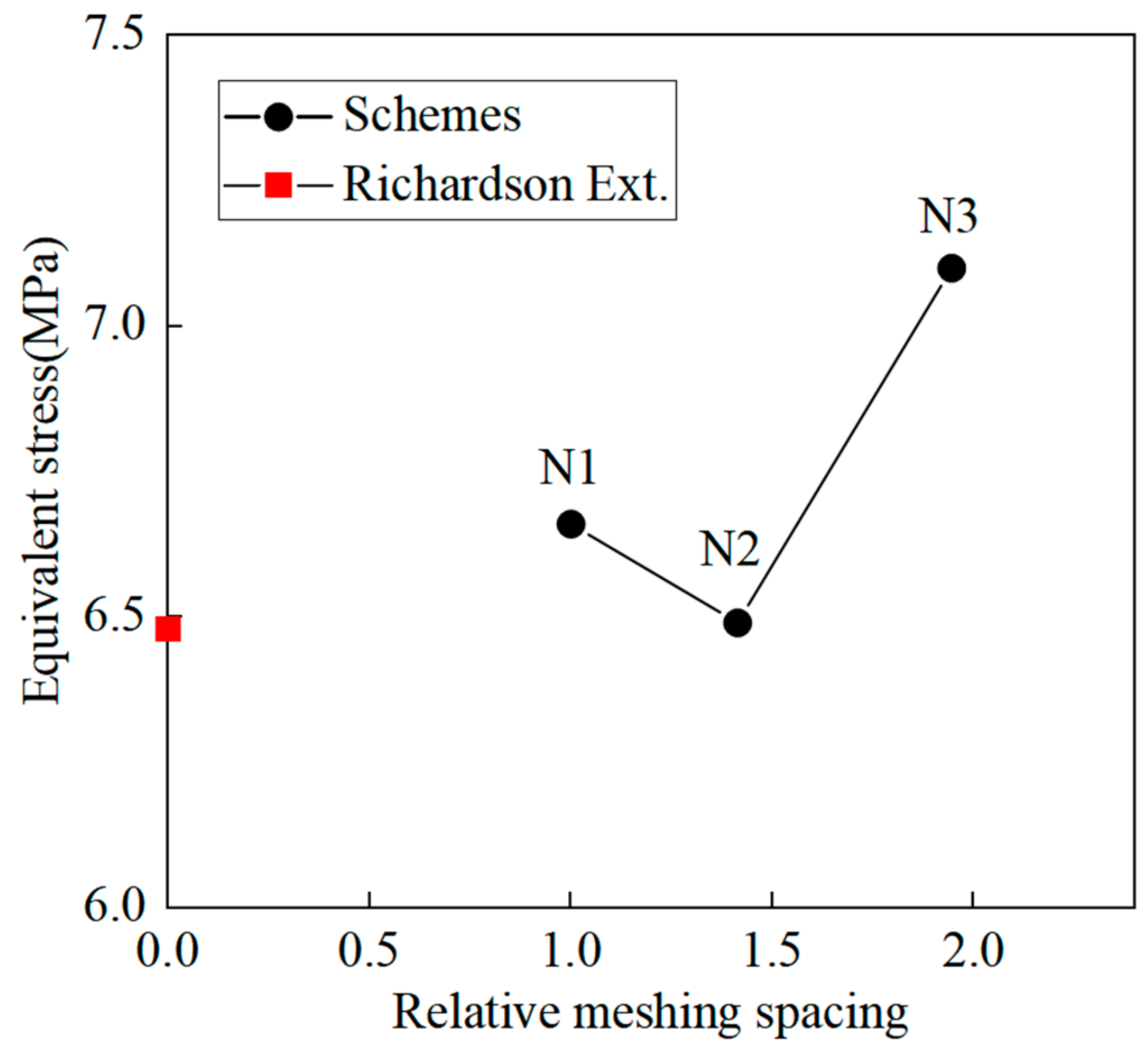
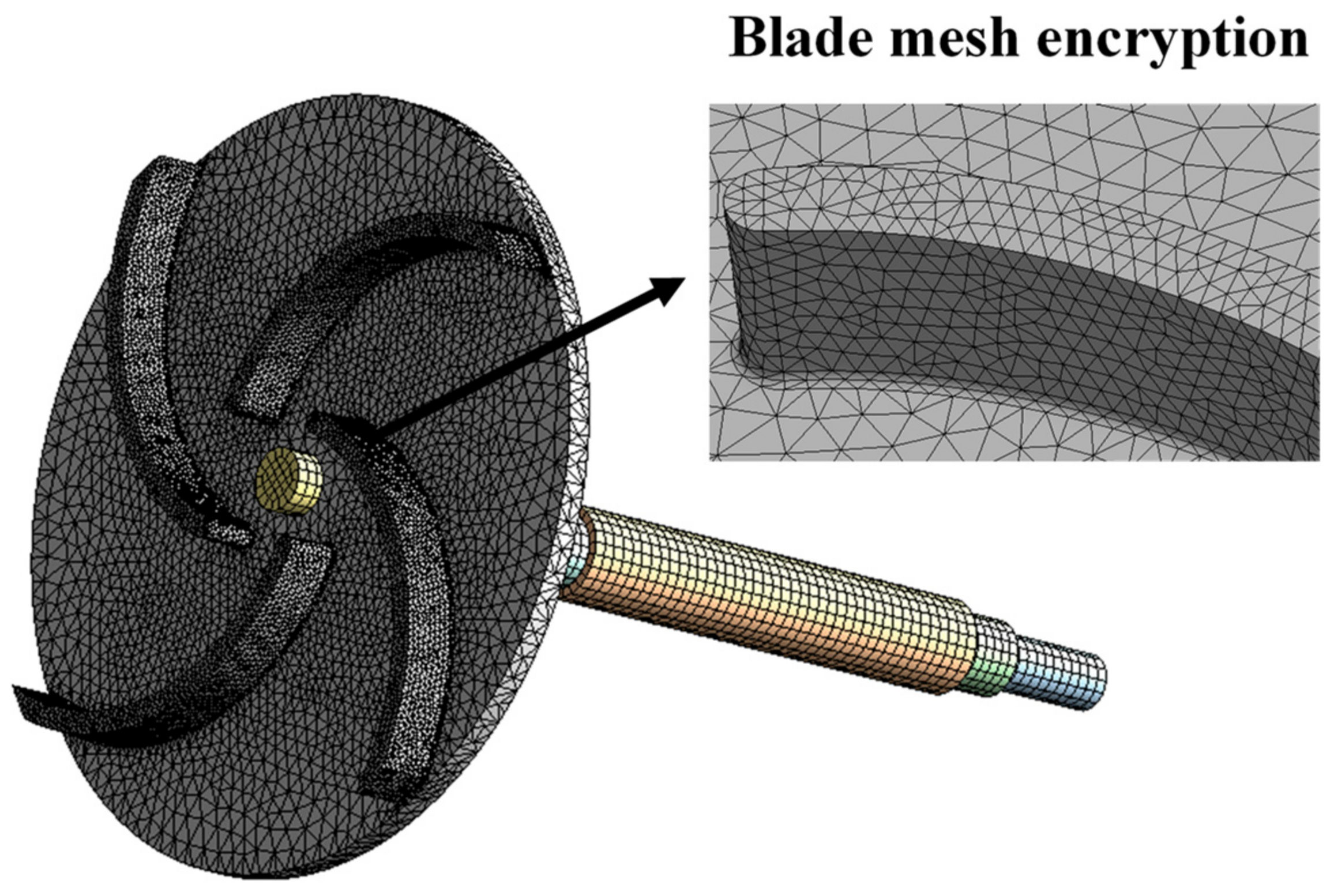
2.3. Meshing and Mesh Independence Verification

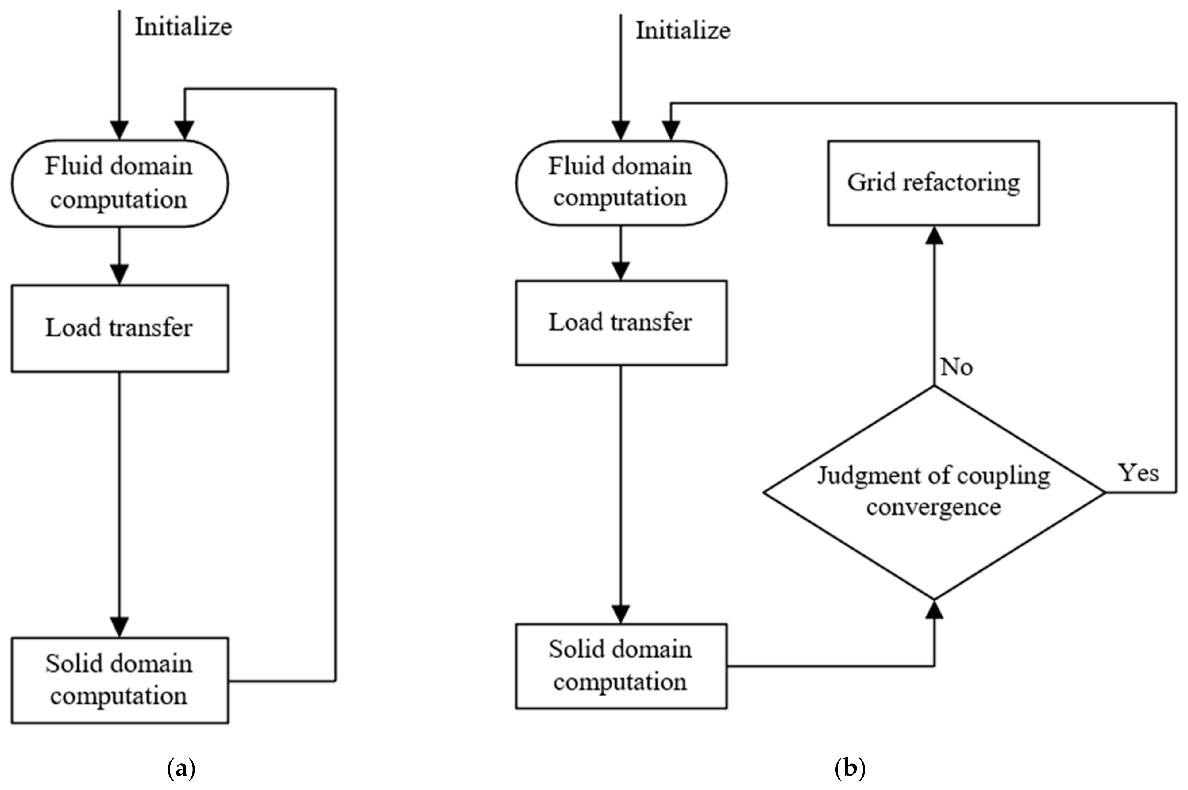
The impeller domain is divided into a hexahedral structured mesh using the commercial software TurboGrid2020, and the boundary layer is encrypted to ensure that more details of the internal flow field structure and pressure distribution characteristics are accurately captured. The inlet section and the volute area are divided into a tetrahedral unstructured mesh using the commercial software ICEM2020. The cut-water is also encrypted to capture the pressure distribution at the cut-water. As shown in

Table 2. Mesh independence check.

Mesh Scheme	Inlet	Impeller	Volute	Total
1	408,677	1,547,700	553,876	2,510,253
2	222,608	1,127,191	315,098	1,664,897
3	244,675	823,320	267,567	1,335,562
4	157,589	690,370	208,674	1,056,633
5	145,243	478,456	273,945	897,644

, for the fluid domain of the objective pump, five different mesh schemes with different grid numbers are carried out. The calculation accuracy of each mesh scheme is verified by comparing the pump head. Figure 2 shows the change in the head value with different numbers of grids, where the parameter N is the number of grid points. It can be seen in Figure 2 that the number of grid points has little effect on the pump head. Figure 3 shows the residuals of the head calculation under each mesh scheme. It can be seen that the predicted value of the head fluctuates around the average value and that the fluctuation range is small. In Figure 3, δ is the residual between the corresponding head of each grid scheme and the mean value of the corresponding head of all grid schemes. It can be calculated using Equation (10):

$$\delta =H_i-H_{ave}$$

(10)

H_i is the head corresponding to each grid scheme (i = 1, 2,…, 5), and H_ave is the average head value of all grid schemes. In summary, mesh scheme 2, with a total of 1,664,897 grid points, is selected as the final calculation grid, and the mesh details are shown in Figure 4. The y+ value distribution is shown in Figure 5, and it meets the accuracy requirements.

2.4. One-Way FSI

A one-way FSI transfers the flow field results calculated by CFD to the structural field through the coupling surface without considering the reaction of the structural deformation to the flow field [29,30]. Thus, the computational cost of a one-way FSI is much lower than that of a two-way FSI.

The solid material used in this study is structural steel. The material density is 7850 kg/m³, the Young’s modulus is 2 × 10¹¹ Pa, and Poisson’s ratio is 0.3. The structural field load application settings are shown in Figure 6. Considering the centrifugal pump impeller and shafting as a whole, a cylindrical surface constraint is imposed at the position of the two bearings, and a centrifugal force constraint is imposed on the entire solid structure. The entire one-way coupling calculation is carried out in the ANSYS CFX and Static Structural modules of ANSYS Workbench to analyze the displacement and stress of the structure under the corresponding load. The linear analysis equations of structural statics are as follows [31]:

$$[K]\left\{x\right\}=\left\{F\right\}$$

(11)

where [K] is the stiffness matrix; {x} is the displacement vector; and {F} is the force vector.

$$\sigma =[B][D]\left\{x\right\}$$

(12)

where σ is the stress matrix; [B] is the elastic matrix; and [D] is the strain matrix.

According to the fourth strength theory, the Mises equivalent stress can be calculated using Equation (13):

$${\sigma }_e=\sqrt{\frac{1}{2}\left[{\left({\sigma }_1-{\sigma }_2\right)}^2+{\left({\sigma }_2-{\sigma }_3\right)}^2+{\left({\sigma }_3-{\sigma }_1\right)}^2\right]}$$

(13)

where σ₁, σ₂, and σ₃ are three mutually perpendicular principal stresses at an action point; σ_e is the Mises equivalent stress; and the unit is Pa.

The grid independence check method based on the Richardson extrapolation proposed by Celik et al. [32] is used to analyze the grid independence of three sets of grids with different densities (N1 < N2 < N3), where N1 = 22,692, N2 = 63,819, N3 = 166,639, and equivalent stress is taken as the key indicator of grid independence. The convergence results of each grid scheme are shown in Figure 7. Considering the results of the grid convergence analysis and the actual computing resources, the second grid scheme (N2, with a grid number of 63,819) is selected as the final computing grid in this research. A mesh detail diagram is shown in Figure 8.

2.5. Two-Way FSI

A two-way FSI considers both the influence of the flow field structure on the structural deformation and the reaction of the structural deformation to the internal flow [33]. The two transfer and exchange data through the FSI surface, so the result of the two-way FSI is closer to the actual situation. A flow chart of a two-way FSI is shown in Figure 9b. The two-way FSI is realized through the coupling of Transient Structural and ANSYS CFX. The meshing is identical to that of the one-way FSI. The difference is that the FSI surface needs to be added to the structural field. By turning off the automatic time step in the settings, the time step setting is consistent with the flow field and each time step is 0.000476 s. Three monitoring points were installed in the area where there may be large deformation displacement to monitor the change in deformation displacement over time. Equation (14) is the expression of the linear differential equation of structural dynamics:

$$[M]\left\{\ddot{u}\right\}+[C]\left\{\dot{u}\right\}+[K]\left\{u\right\}=\{F(t)\}$$

(14)

where [M], [C], and [K] are the structural mass matrix, damping matrix, and stiffness matrix, respectively, and {F(t)} is the external structure load vector.

2.6. Modal Analysis Methods

Modal analysis is a commonly used dynamic analysis method in the field of fluid machinery simulation. It is mainly used to analyze the natural frequency and mode shape of a structure. The natural frequency of a structure is related to many factors, such as the material used by the structure itself, the operating state, and the magnitude of the load. When the operating frequency of a centrifugal pump is the same as the natural frequency of a structure, a large structural deformation will occur due to structural resonance, which will affect the safety and stability of pump operation in severe cases. Hence, obtaining a natural frequency of the pump and its mode shape via modal analysis can provide a reference for the design of the centrifugal pump.

The linear differential equation of structural dynamics is the same as Equation (14). For the modal analysis, the overall load matrix of the structure is {F(t)} = 0, and the damping of the structure can be ignored; that is, [C] = 0. Therefore, the structural dynamic linear differential equations can be expressed using Equation (15):

$$[M]\left\{\ddot{u}\right\}+[K]\left\{u\right\}=\left\{0\right\}$$

(15)

From the free vibration of the structure as simple harmonic vibration, the displacement function (Equation (16)) can be obtained:

$$x=x\sin (\omega t)$$

(16)

The dynamic equation of modal analysis can be obtained as Equation (17):

$$\left([K]-{\omega }^2[M]\right)\left\{x\right\}=\left\{0\right\}$$

(17)

To solve Equation (17), the natural frequency and the mode shape of the structure are the eigenvalues and eigenvectors, and the structure must be linear.

3. Result Analysis

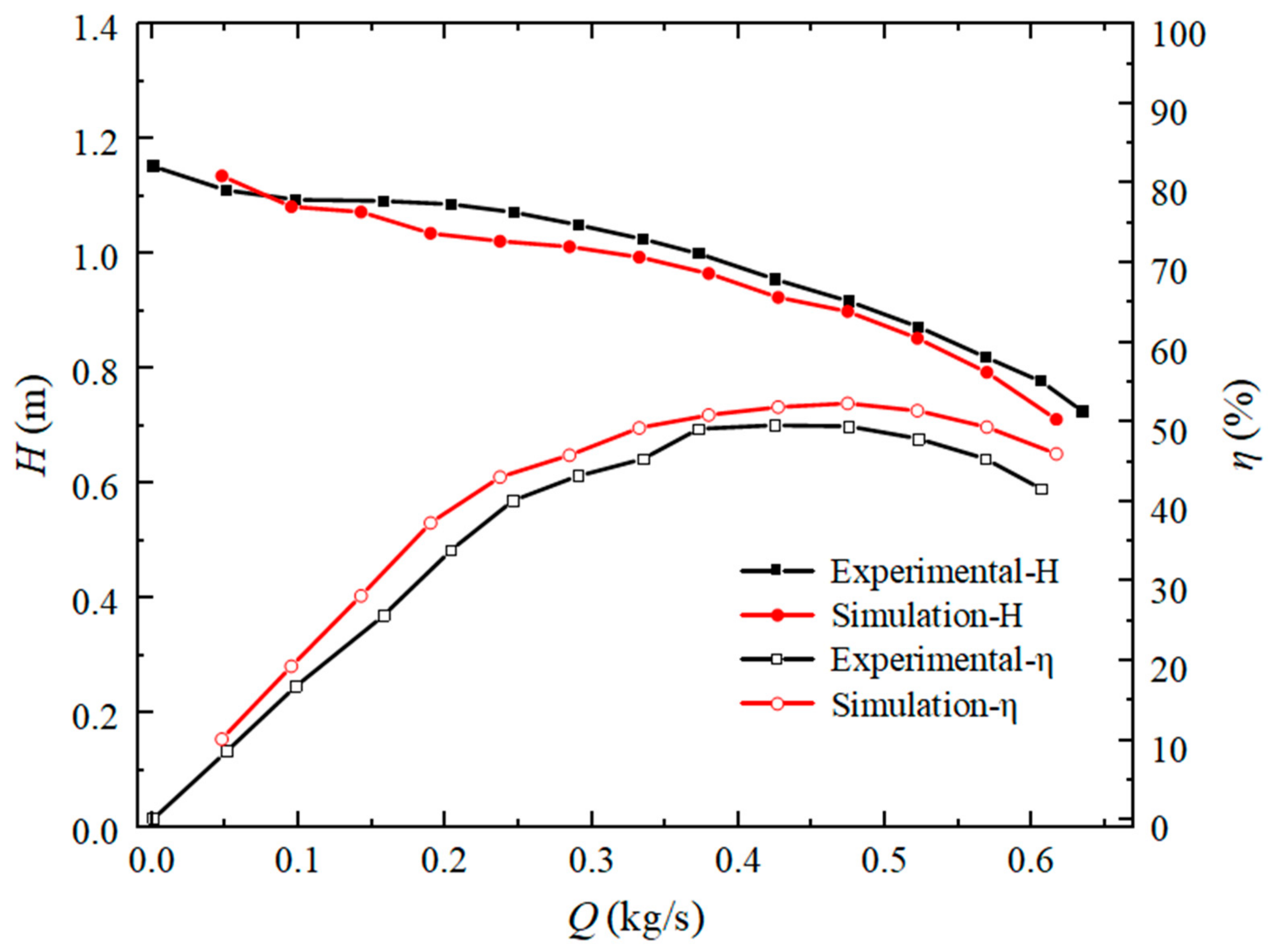
3.1. Analysis of External Characteristics

In order to obtain the changing values of the external characteristics, a steady calculation was set every 0.1 Q_d between 0.1 and 1.3 Q_d. Then, the H-Q and η-Q curves were drawn and compared with the experimental data of the external characteristics of the prototype pump. The results are shown in Figure 10.

It can be seen that the simulation results are consistent with the experimentally measured results. The simulation head is slightly lower than the experimental head, and the maximum error does not exceed 3.5%. The simulation value at each flow rate point in the efficiency curve is higher than the experimental value. The difference is larger under part-load flow rate conditions but smaller under the design condition. The difference increases slightly when the design condition is exceeded, but the maximum relative error does not exceed 10%. This is because the structure and size of the model are consistent with those in the literature, but there may be a slight difference between the blade arc transition mode and the experimental model, which may result in a lower head value, when calculated via numerical methods, compared to the experimental value. In general, the calculation model can accurately predict the performance of the pump, so the next step of FSI analysis can be carried out.

The two-way FSI considers the interaction of the fluid and the structure, and the structural deformation affects the internal flow state, which in turn affects the external characteristics of the pump. Thus, it is necessary to analyze the influence of the FSI on the external characteristics of the centrifugal pump. Figure 11 shows a comparison of the external characteristics of the low-specific-speed centrifugal pump under the action of the two-way FSI and non-coupling. It compares the last two cycles of the unsteady results of the flow field calculation with the two-way FSI data. It indicates that the change laws of the external characteristic curves in the uncoupled and two-way FSI states are basically the same, and there are four peaks in each rotation cycle, which is the same as the number of blades. It indicates that with the rotation of the impeller, the rotor–stator interaction at the cut-water has a great influence on the external characteristics of the centrifugal pump.

The peak predicted values of the FSI head and efficiency are larger than the head efficiency value under the non-coupling condition, and the two-way FSI structure has a large fluctuation range, which is affected by the dual effects of the FSI and the rotor–stator interaction. By calculating the average values of the two results, the average head of the uncoupled result is 0.895 m, and the average head of the two-way coupling is 0.911 m. The experimental head of the pump under the design condition is 0.917 m. The errors for uncoupling and two-way coupling are 2.4% and 0.6%, respectively, which meet the calculation requirements. Thus, the two-way FSI calculation results are closer to the experimental results, and the results are more reliable.

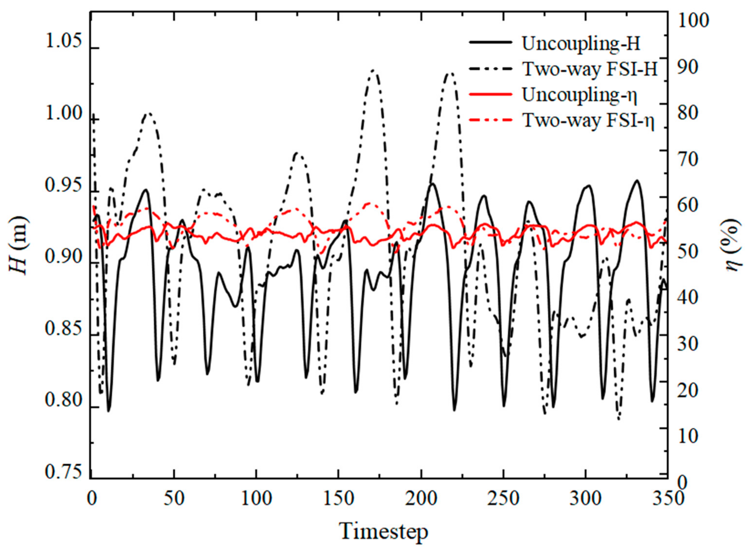
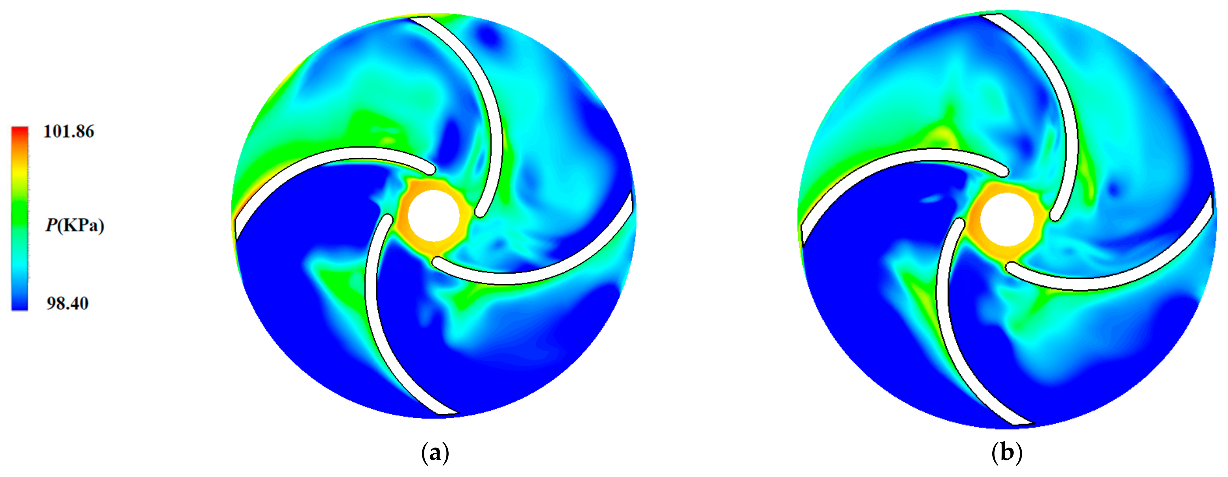
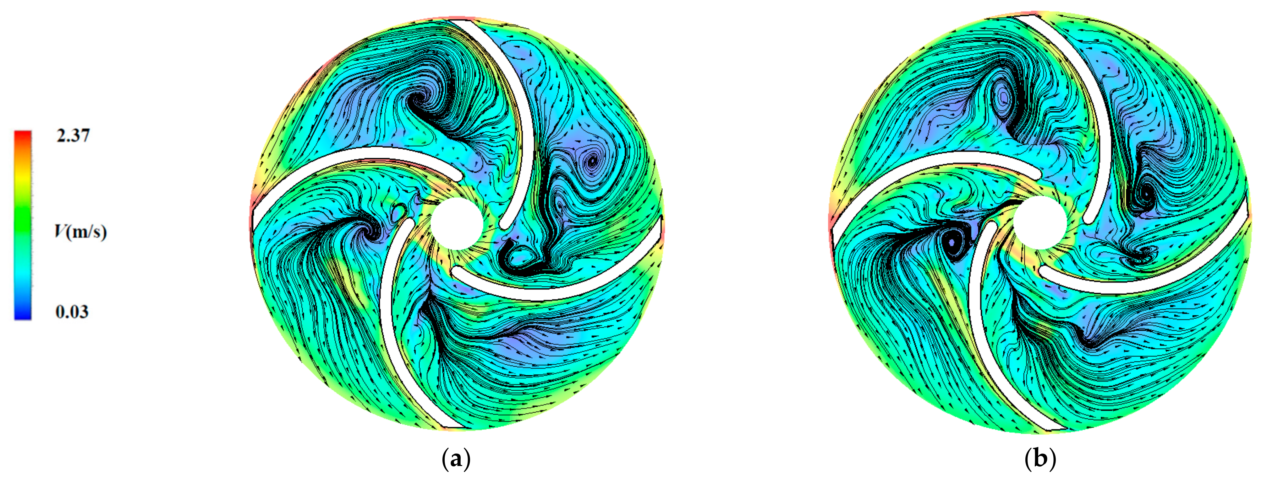
3.2. Influence of FSI on Flow Field and Structural Field

By analyzing the calculation results of the unsteady flow field and the two-way FSI flow field, the influence of the FSI on the internal flow field of the low-specific-speed centrifugal pump is analyzed. The results of the last time step of the unsteady calculation are selected to compare with the results of the two-way FSI.

Figure 12 shows the total pressure distribution in the pump before and after the FSI. It can be seen that the two-way FSI has little effect on the internal total pressure distribution of the low-specific-speed centrifugal pump and that the pressure on the pressure surface of the blade is greater than the pressure on the suction surface of the blade. Figure 13 shows the velocity streamline distribution in the pump before and after the FSI. It can be observed that there are vortices of different scales within the centrifugal pump. Flow instability is a common phenomenon inside centrifugal pumps, and through numerical simulation, this physical instability in the flow can be clearly observed. It indicates that after considering the FSI, the internal streamline changes are not obvious, and the velocity distribution is basically the same, but the prediction of the internal stall vortex is more accurate. The velocity distribution of the pressure surface and the suction surface of the blade changes. The reason for this is the obvious influence of the velocity of the blade as the FSI surface exchanges the flow field and the structural field.

Figure 14 shows the pressure distribution at the cut-water before and after the FSI. It shows that the pressure at the cut-water after considering the FSI is higher than that without considering the FSI because the prediction of the rotor–stator interaction at the cut-water between the impeller and the volute is more accurate after considering the FSI. Therefore, the pressure value of the cut-water predicted by the coupling is larger than that of the uncoupling.

Figure 15 shows the distribution of the total deformation of the impeller in the cases of the one-way FSI and the two-way FSI. The deformation of the impeller increases gradually from the inlet to the outlet, and the maximum deformation occurs at the outlet of the impeller. In the case of the two-way FSI, the maximum deformation of the impeller presents an eccentric distribution, and the total deformation of the impeller in the two-way FSI is slightly larger than that in the one-way condition. Therefore, the FSI method has a certain influence on the maximum deformation distribution of the impeller.

The equivalent stress distributions of the impeller using different coupling methods are shown in Figure 16. They indicate that different coupling methods have a certain influence on the equivalent stress distribution of the impeller. The two-way coupling predicts that the maximum equivalent stress results are larger than the one-way coupling results, and the maximum equivalent stress occurs at the position where the impeller inlet and the rear cover are connected, indicating that the possibility of a structural fracture is greatest here. This result can provide a reference for the subsequent improvement of impeller stress.

3.3. Coherence Analysis between Structural Field and Flow Field

In the field of FSI research, investigating the coherence between structural performance and pressure pulsations in a flow field is of significant importance. This is a complex area of study that garners considerable attention in both engineering and scientific domains. Delving deep into the intricate relationship between fluid dynamics and structural mechanics to unveil the potential impacts of the flow environment on engineering structural performance is crucial. This research has substantial implications for the optimization and redesign of centrifugal pump performance.

Therefore, based on unsteady simulations of the low-specific-speed centrifugal pump, this study employed a two-way FSI approach to compute the maximum deformation and the maximum equivalent stress in the structural field. The time step of the structural field was synchronized with the flow field calculation. This yielded time-dependent curves for the maximum deformation and the maximum equivalent stress. Simultaneously, pressure pulsation data from the monitoring points in the flow field were recorded over time. Signal coherence analysis was then utilized to examine the coherence between the pressure pulsation data at various points and the maximum deformation and maximum equivalent stress in the structural field. Specifically, the signal coherence between the pressure pulsation data and the maximum equivalent stress data, between the pressure pulsation data and the maximum deformation data, and between the maximum deformation and the maximum equivalent stress data was computed. If we consider two time series signals, x(t) and y(t), the cross-spectral density function C_xy(f) between them can be expressed as

$$C_{xy}\left(f\right)=\frac{|S_{xy}(f){|}^2}{S_{xx}\left(f\right)S_{yy}\left(f\right)}$$

(18)

Here, f represents the frequency; S_xy(f) denotes the cross-power spectral density between x(t) and y(t); and S_xx(f) and S_xy(f) are the auto-power spectral densities of x(t) and y(t), respectively.

Figure 17 shows the changing trends of the maximum deformation and maximum equivalent stress over time. The maximum deformation exhibits significant fluctuations within one rotation cycle of the impeller, while the maximum equivalent stress undergoes one oscillation cycle within a single rotational period, initially increasing and then decreasing. Figure 18 illustrates the variations in the pressure pulsation monitoring data at different points within the flow field. Due to the effects of the rotor–stator interaction, the three monitoring points between the impeller and the volute exhibit larger pressure pulsation amplitudes, while the two monitoring points inside the channel show smaller pulsation amplitudes and follow different pulsation patterns.

Figure 19 displays the distribution patterns of the coherence coefficients between the pressure pulsations at the five monitoring points and the maximum equivalent stress and maximum deformation in the structural field as a function of frequency. C_ED represents the coherence coefficient between the maximum equivalent stress and the maximum deformation, while C_DP1 and C_EP1, respectively, represent the coherence coefficients between the maximum deformation, maximum equivalent stress, and the pressure pulsations at monitoring point P1. From the figure, it can be observed that the distribution patterns of the coherence coefficients between the pressure pulsations and the deformation and equivalent stress in different locations inside the centrifugal pump vary, but they exhibit good consistency in certain frequency ranges. The coherence coefficients between the pressure pulsations at points P1 and P2 at the interface of the impeller and volute as well as the signals of the maximum equivalent stress and maximum deformation are relatively high. Based on the rotational speed calculation of the impeller, the rotating frequency of the impeller is 11.67 Hz, and the blade passing frequency is 46.68 Hz. It can be observed that the peak values of the coherence coefficients at various frequencies coincide with the rotational frequency of the impeller and the blade passing frequency. This indicates strong coherence between the interaction of the impeller and the volute and the structural performance of the impeller. When the fluid within the flow field passes through the interface into the volute, it generates significant pulsations. These pulsations are then transmitted to the structural field, leading to fluctuations in the maximum deformation and the maximum equivalent stress.

The coherence coefficients C_DP5 and C_EP5 at point P5 near the cut-water of the volute exhibit significant reductions in coherence at various frequencies. The points S1 and S3 within the flow passage of the impeller only show relatively high coherence coefficients (C_DS1, C_ES1, C_DS3, and C_ES3) at some low frequencies below 300 Hz, indicating lower coherence between the pressure pulsations caused by unstable flow structures within the flow passage of the impeller and the stress–strain signals in the structural field. Furthermore, upon examining the distribution of the coherence coefficients at all points, it is observed that at frequencies around 93 Hz and 233 Hz, the pressure pulsations from the flow field and the maximum deformation signals in the structural field both have peaks in their coherence coefficients. These frequencies correspond to two times and five times the blade passing frequency, indicating strong coherence between the two signals at these specific frequencies.

3.4. FSI Modal Analysis

Table 3. Comparison of modal frequencies with and without prestress.

Order (n)	1	2	3	4	5	6
With prestress (Hz)	232.93	275.27	275.71	841.90	843.09	1104.5
Without prestress (Hz)	232.92	275.98	276.41	840.51	841.70	1104.5

shows a comparison of the first six modal frequencies of the impeller with and without prestress. The rotor is affected by the excitation effect of the fluid pressure pulsation, and the frequency difference is 1.39 Hz. At the same time, under both calculation modes, the first-order mode frequency of the impeller coincides with five times the blade passing frequency, which is consistent with the results of the previous analysis of the coherence between the flow field and structural field signals mentioned earlier.

Figure 20 and Figure 21 show the modal distribution of the first six orders before and after applying prestress. Compared with the mode shape of the dry modal impeller, the modal distribution does not change significantly. However, combined with the comparison of the frequencies of each order, it can be seen that the vibration amplitude of the impeller under the action of the one-way FSI has a decreasing trend, which indicates that prestress has an inhibitory effect on the vibration of the impeller.

4. Conclusions

In this study, the unsteady flow characteristics in a low-specific-speed centrifugal pump are simulated using the CFD method. The two-way fluid–structure coupling method is used to calculate the flow characteristics of the pump, and the effect of the FSI on the internal flow structure of the centrifugal pump is analyzed. Utilizing two-way fluid–structure coupling, the signal coherence analysis method is employed to analyze the coherence of the signals between the flow field and the structural field. The specific conclusions are as follows:

(1)

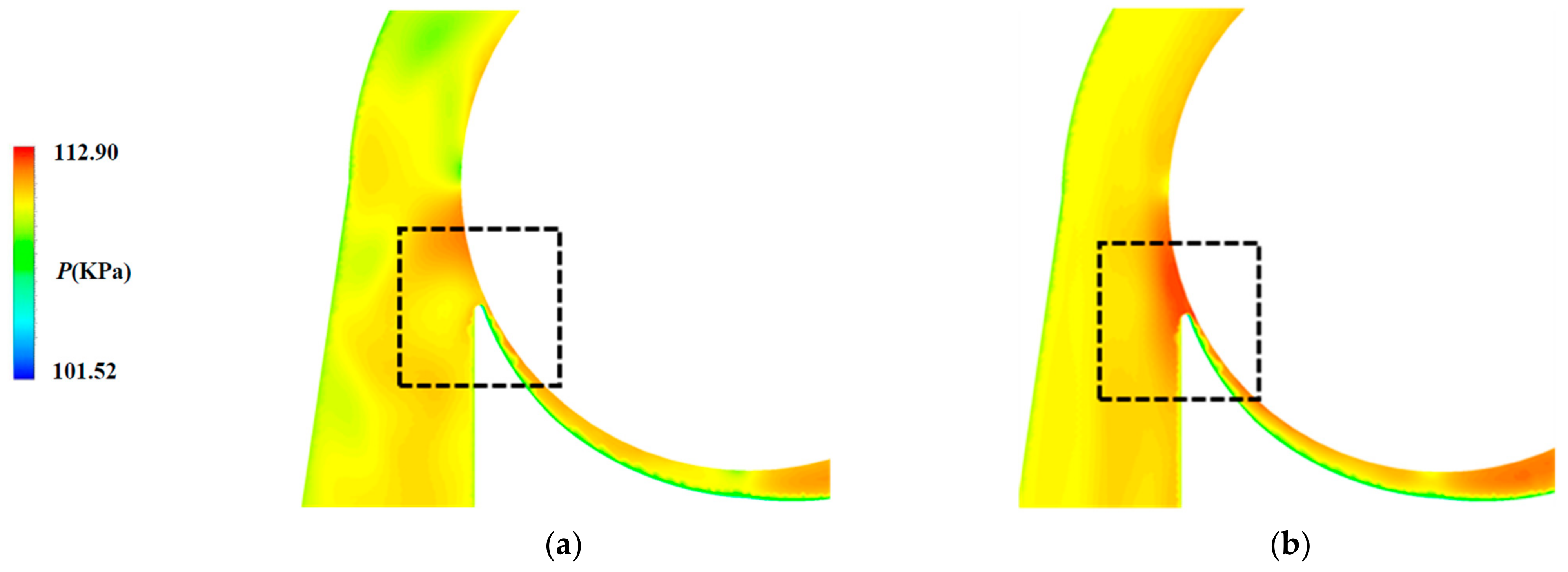
By employing the two-way FSI method, we successfully compute the flow characteristics of the centrifugal pump, providing a comprehensive revelation of the impact of the FSI on the internal flow structure. This contributes to a more comprehensive understanding of the performance and behavior of the pump. The FSI has a greater influence on the pressure distribution at the cut-water. This is because the prediction of the rotor–stator interaction at the cut-water between the impeller and the volute is more accurate after considering the FSI. Therefore, in designs and optimizations involving the cut-water region, it is necessary to pay attention to this location. Through the comparison of the external characteristics before and after the two-way FSI with the experimental values, it is found that the error between the predicted and experimental values of the external characteristics is smaller after the two-way FSI and that the prediction is more accurate.

(2)

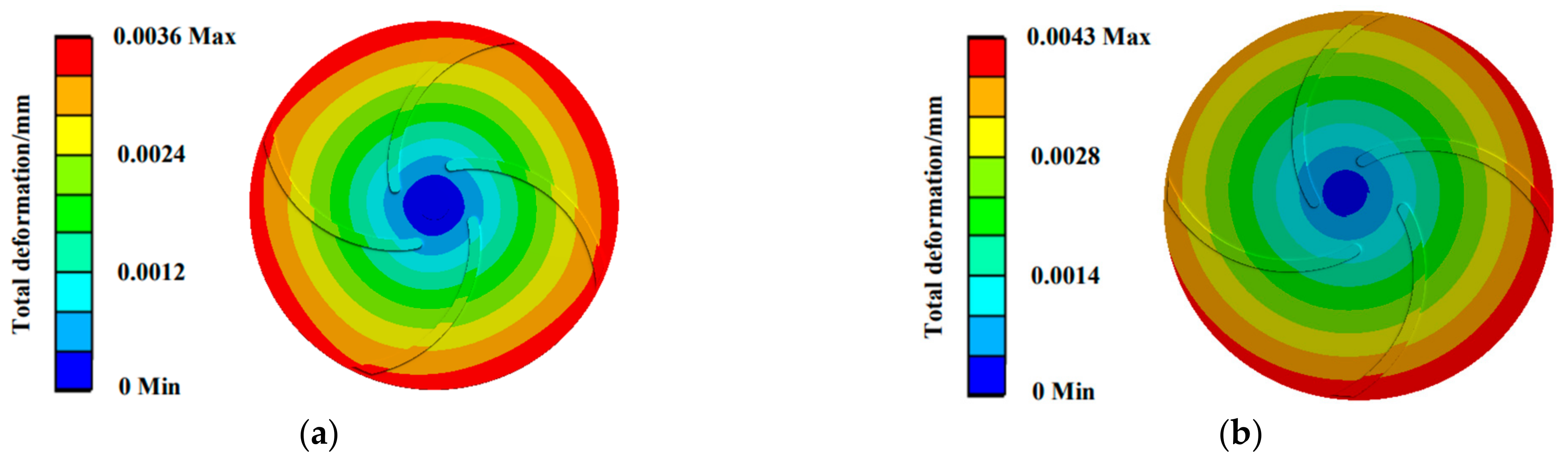
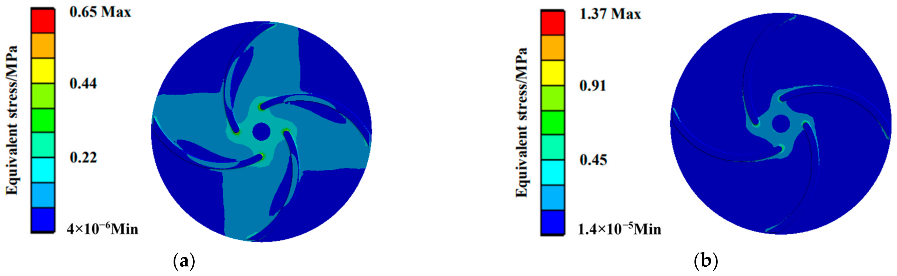
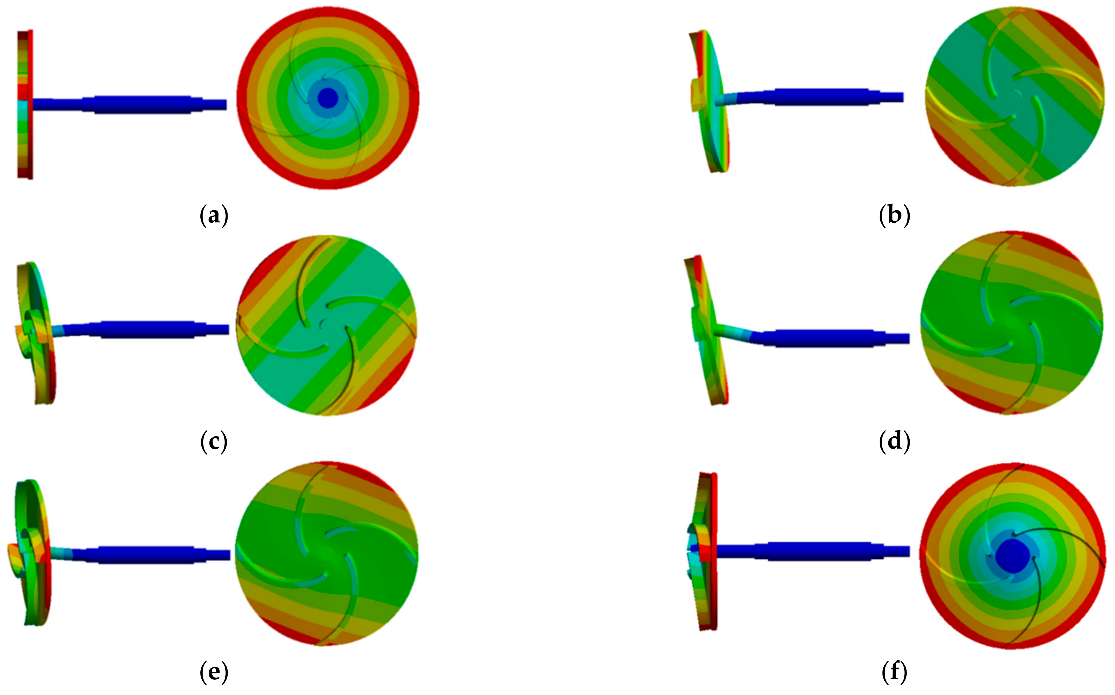
Different coupling methods have a certain influence on the impeller stress and deformation. Using the two coupling methods, the maximum deformation is located at the outlet of the impeller, and the maximum equivalent stress is located at the connection between the leading edge of the impeller inlet and the impeller hub. This underscores that the critical region of force on the impeller of the low-specific-speed centrifugal pump experiences the maximum stress and may be an area that requires particular attention. The results of the two-way FSI are larger than those of the one-way FSI. However, considering that the two-way FSI requires a lot of computing resources, the results of the one-way FSI can be used when the deformation of the research object is not large. This balance can be found between computational efficiency and result accuracy. In the case of one-way coupling and uncoupling, the first six modal frequencies of the impeller are similar, but the fourth and fifth orders have a great influence, and the frequency difference is 1.39 Hz. This highlights the importance of selecting the appropriate coupling method at specific modal frequencies.

(3)

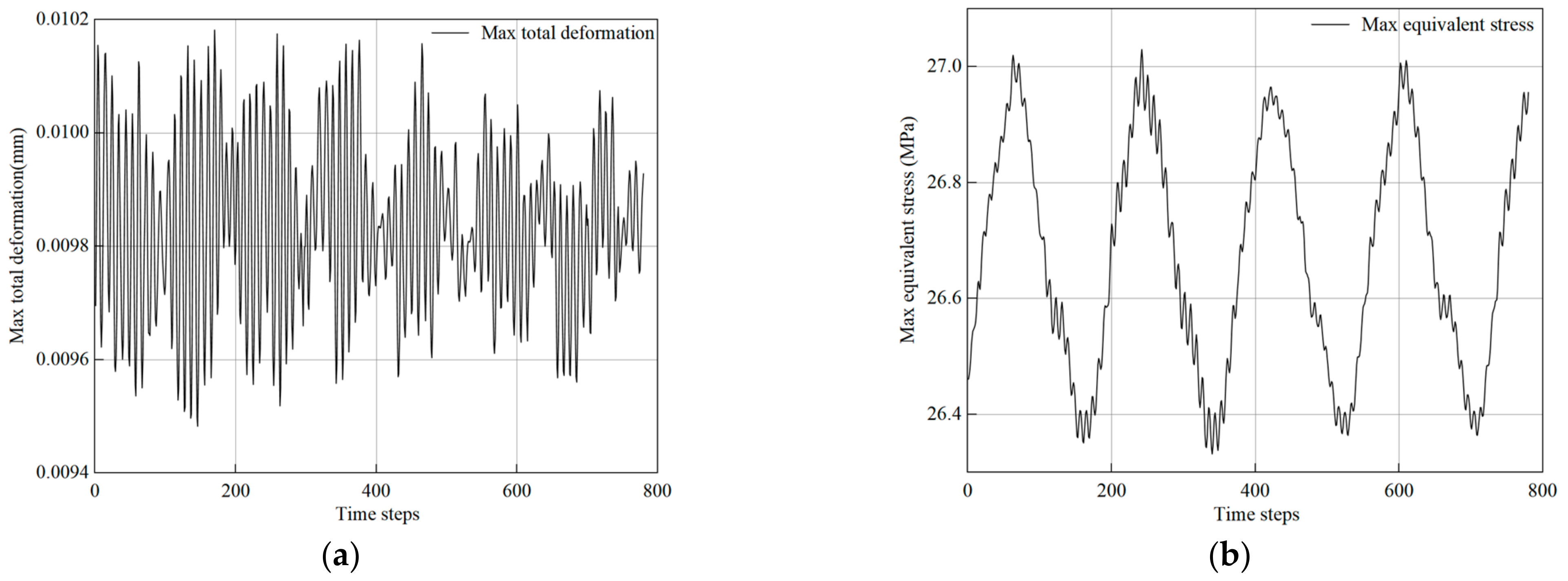
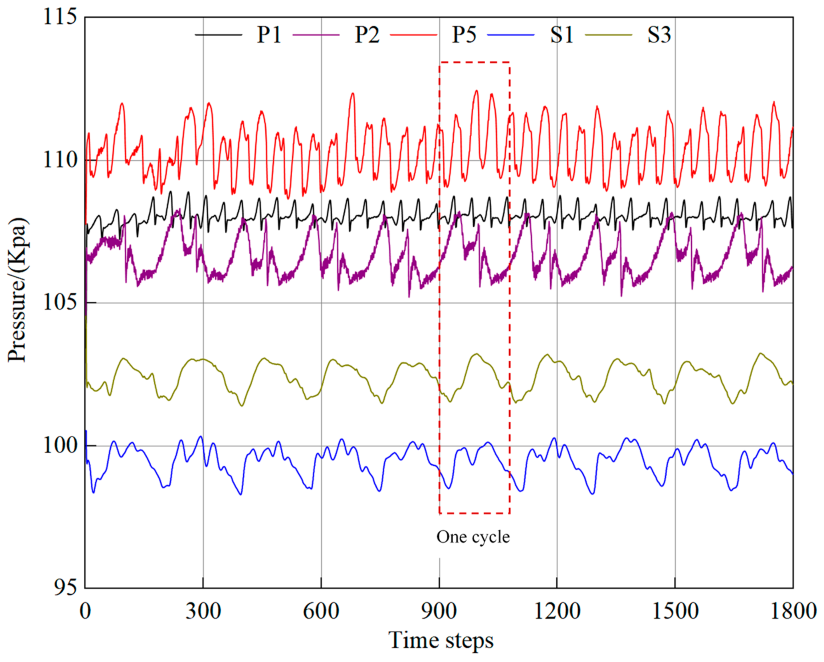
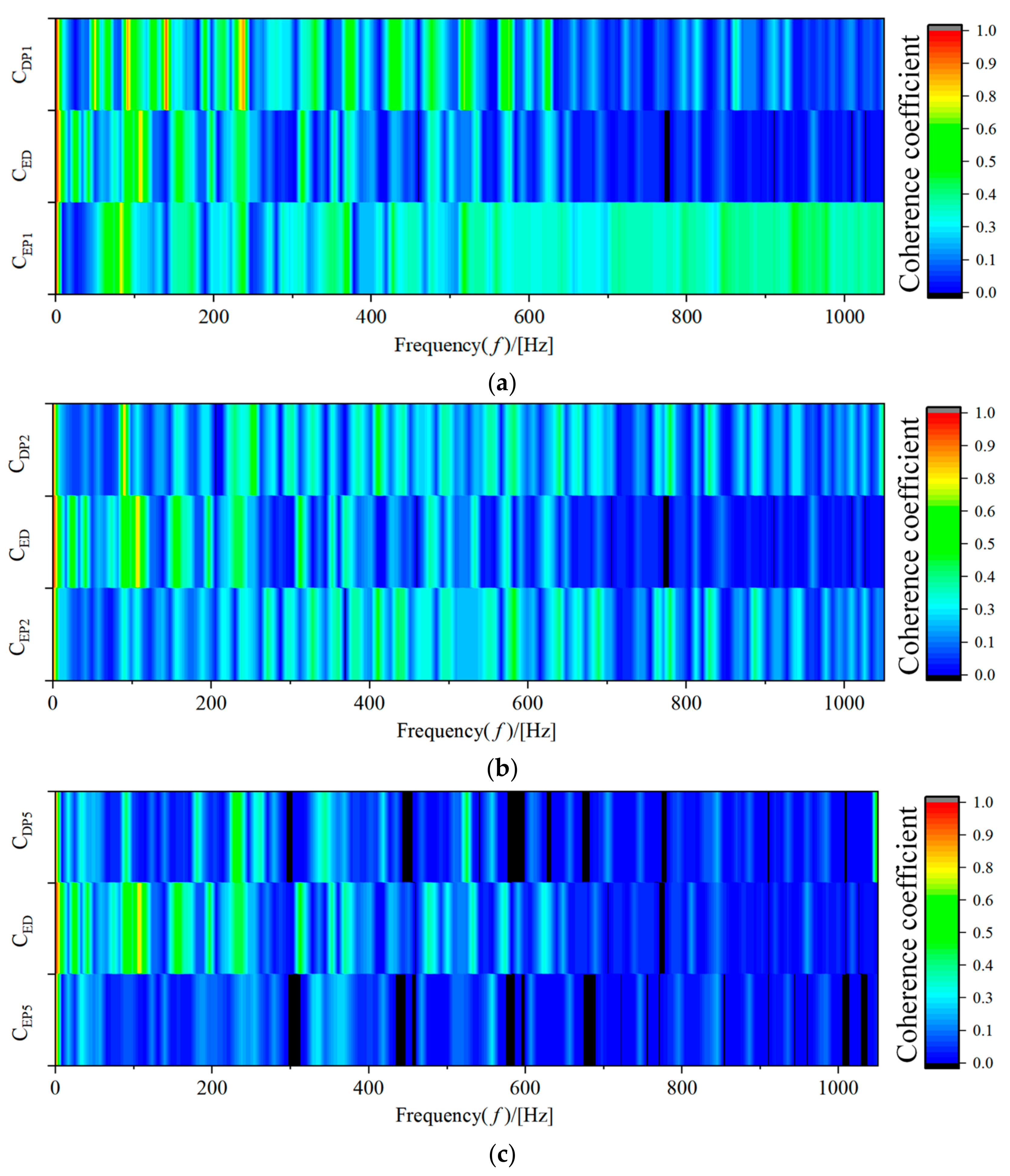
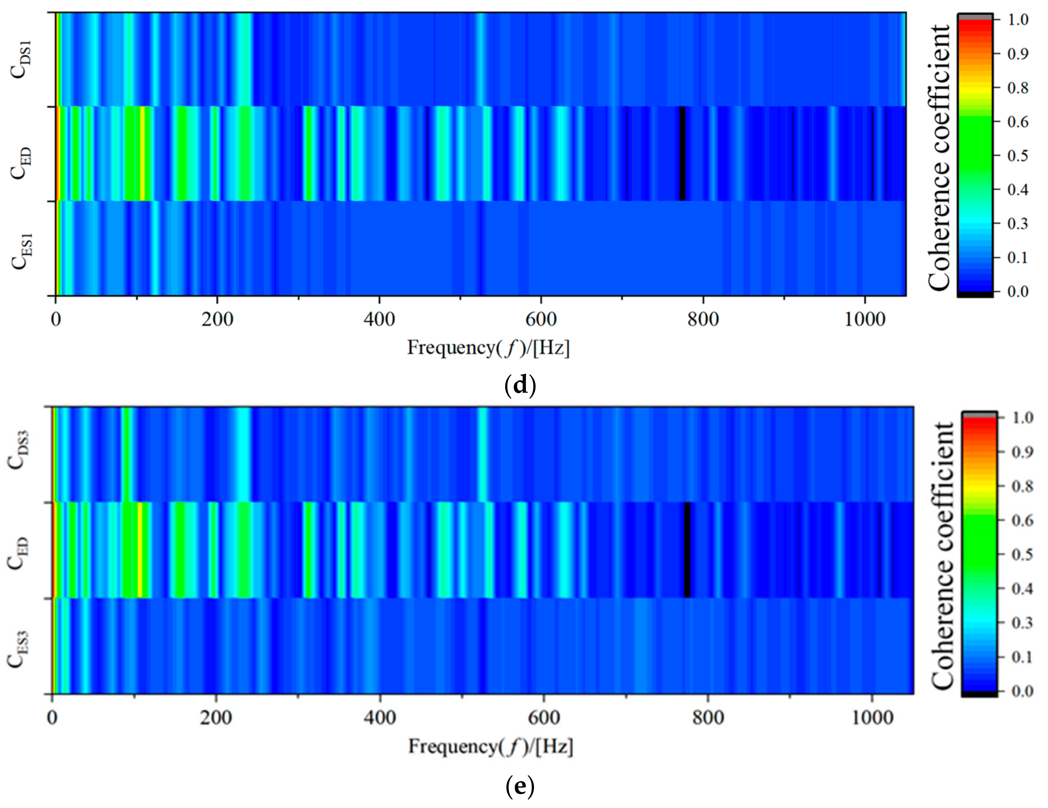
Through signal coherence analysis, we delved into the correlation between the flow field and the structural field, providing a perspective that offers a deeper understanding of the FSI mechanism. The pressure pulsation signals at the interface of the volute and the impeller exhibit high coherence with the signals of maximum equivalent stress and maximum deformation. The frequencies at which these coherence coefficients have peak values align with the rotational speed of the impeller and the blade passing frequency. This indicates that the rotor–stator interaction between the interface of the volute and the impeller leads to significant variations in the structural field performance. On the other hand, the pressure pulsation signals originating from the unstable flow structures within the flow path of the impeller show weaker coherence with the stress and strain signals in the structural field. At specific frequencies of approximately 93 Hz and 233 Hz, all monitoring points display strong coherence between the flow field signals and the maximum deformation signals. These frequencies correspond to twice and five times the blade passing frequency. These findings contribute to a better understanding of the interaction between the fluid and the structure in low-specific-speed centrifugal pumps, offering valuable insights for improved design and performance predictions.

References

1. Zhang, F.; Appiah, D.; Hong, F.; Zhang, J.; Yuan, S.; Adu-Poku, K.A.; Wei, X. Energy loss evaluation in a side channel pump under different wrapping angles using entropy production method. Int. Commun. Heat Mass Transf. 2020, 113, 104526. [Google Scholar] [CrossRef]
2. Šavar, M.; Kozmar, H.; Sutlović, I. Improving centrifugal pump efficiency by impeller trimming. Desalination 2009, 249, 654–659. [Google Scholar] [CrossRef]
3. Wang, C.; Zhang, Y.; Hou, H.; Yuan, Z. Theory and application of two-dimension viscous hydraulic design of the ultra-low specific-speed centrifugal pump. Proc. Inst. Mech. Eng. Part A J. Power Energy 2020, 234, 58–71. [Google Scholar] [CrossRef]
4. Zhang, Y.-L.; Zhu, Z.-C.; Li, W.-G. Experiments on transient performance of a low specific speed centrifugal pump with open impeller. Proc. Inst. Mech. Eng. Part A J. Power Energy 2016, 230, 648–659. [Google Scholar] [CrossRef]
5. Choi, Y.-D.; Nishino, K.; Kurokawa, J.; Matsui, J. PIV measurement of internal flow characteristics of very low specific speed semi-open impeller. Exp. Fluids 2004, 37, 617–630. [Google Scholar] [CrossRef]
6. Chabannes, L.; Štefan, D.; Rudolf, P. Effect of Splitter Blades on Performances of a Very Low Specific Speed Pump. Energies 2021, 14, 3785. [Google Scholar] [CrossRef]
7. Liang, D.; Yuqi, Z.; Houlin, L.; Cui, D.; Vladimirovich, G.D.; Yong, W. The effect of front streamline wrapping angle variation in a super-low specific speed centrifugal pump. Proc. Inst. Mech. Eng. Part C J. Mech. Eng. Sci. 2018, 232, 4301–4311. [Google Scholar] [CrossRef]
8. Jafarzadeh, B.; Hajari, A.; Alishahi, M.; Akbari, M. The flow simulation of a low-specific-speed high-speed centrifugal pump. Appl. Math. Model. 2011, 35, 242–249. [Google Scholar] [CrossRef]
9. Sakthivel, N.; Sugumaran, V.; Babudevasenapati, S. Vibration based fault diagnosis of monoblock centrifugal pump using decision tree. Expert Syst. Appl. 2010, 37, 4040–4049. [Google Scholar] [CrossRef]
10. Yanhua, W.; Longlong, H.; Yong, L.; Jingsong, X. Comparative analysis of cycloid pump based on CFD and fluid structure in-teractions. Adv. Mech. Eng. 2020, 12, 1687814020973533. [Google Scholar] [CrossRef]
11. Pellegri, M.; Manne, V.H.B.; Vacca, A. A simulation model of Gerotor pumps considering fluid–structure interaction effects: Formulation and validation. Mech. Syst. Signal Process. 2020, 140, 106720. [Google Scholar] [CrossRef]
12. Adamkowski, A.; Henke, A.; Lewandowski, M. Resonance of torsional vibrations of centrifugal pump shafts due to cavitation erosion of pump impellers. Eng. Fail. Anal. 2016, 70, 56–72. [Google Scholar] [CrossRef]
13. Ouyang, J.; Luo, Y.; Tao, R. Influence of blade leaning on hydraulic excitation and structural response of a reversible pump turbine. Proc. Inst. Mech. Eng. Part A J. Power Energy 2021, 236, 241–259. [Google Scholar] [CrossRef]
14. Wang, J.; Wang, P.; Zhang, X.; Ruan, X.; Xu, Z.; Fu, X. Research of Modal Analysis for Impeller of Reactor Coolant Pump. Appl. Sci. 2019, 9, 4551. [Google Scholar] [CrossRef]
15. Yin, T.; Pei, J.; Yuan, S.; Osman, M.K.; Wang, J.; Wang, W. FSI analysis of an impeller for a high-pressure booster pump for seawater desalination. J. Mech. Sci. Technol. 2017, 31, 5319–5328. [Google Scholar] [CrossRef]
16. Matlakala, M.E.; Kallon, D.V.; Mogapi, K.E.; Mabelane, I.M.; Makgopa, D.M. Influence of Impeller Diameter on the Performance of Centrifugal pumps. IOP Conf. Ser. Mater. Sci. Eng. 2019, 655, 012009. [Google Scholar] [CrossRef]
17. Mousmoulis, G.; Kassanos, I.; Aggidis, G.; Anagnostopoulos, I. Numerical simulation of the performance of a centrifugal pump with a semi-open impeller under normal and cavitating conditions. Appl. Math. Model. 2020, 89, 1814–1834. [Google Scholar] [CrossRef]
18. Xiao, R.; Wang, Z.; Luo, Y. Dynamic stresses in a francis turbine runner based on FSI analysis. Tsinghua Sci. Technol. 2008, 13, 587–592. [Google Scholar] [CrossRef]
19. Zhang, L.; Wang, S.; Yin, G.; Guan, C. Fluid–structure interaction analysis of fluid pressure pulsation and structural vibration features in a vertical axial pump. Adv. Mech. Eng. 2019, 11, 1–19. [Google Scholar] [CrossRef]
20. Afra, B.; Delouei, A.A.; Tarokh, A. Flow-Induced Locomotion of a Flexible Filament in the Wake of a Cylinder in Non-Newtonian Flows. Int. J. Mech. Sci. 2022, 234, 107693. [Google Scholar] [CrossRef]
21. Delouei, A.A.; Karimnejad, S.; He, F. Direct Numerical Simulation of pulsating flow effect on the distribution of non-circular particles with increased levels of complexity: IB-LBM. Comput. Math. Appl. 2022, 121, 115–130. [Google Scholar] [CrossRef]
22. Jiang, Y.; Yoshimura, S.; Imai, R.; Katsura, H.; Yoshida, T.; Kato, C. Quantitative evaluation of flow-induced structural vibration and noise in turbomachinery by full-scale weakly coupled simulation. J. Fluids Struct. 2007, 23, 531–544. [Google Scholar] [CrossRef]
23. Li, W.; Ji, L.; Shi, W.; Zhou, L.; Jiang, X. FSI study of a mixed-flow pump impeller during startup. Eng. Comput. 2018, 35, 18–34. [Google Scholar] [CrossRef]
24. Kato, C.; Yoshimura, S.; Yamade, Y.; Jiang, Y.Y.; Wang, H.; Imai, R.; Katsura, H.; Yoshida, T.; Takano, Y. Prediction of the noise from a multi-stage centrifugal pump. In Proceedings of the ASME 2005 Fluids Engineering Division Summer Meeting, Houston, TX, USA, 19–23 June 2005; pp. 1273–1280. [Google Scholar]
25. MacPhee, D.W.; Beyene, A. Fluid–structure interaction analysis of a morphing vertical axis wind turbine. J. Fluids Struct. 2016, 60, 143–159. [Google Scholar] [CrossRef]
26. Benra, F.K.; Dohmen, H.J.; Pei, J.; Schuster, S.; Wan, B. A comparison of one-way and two-way coupling methods for numerical analysis of FSIs. J. Appl. Math. 2011, 2011, 1–16. [Google Scholar] [CrossRef]
27. Degroote, J. Partitioned Simulation of Fluid-Structure Interaction Coupling Black-Box Solvers with Quasi-Newton Techniques. Arch. Comput. Methods Eng. 2013, 20, 185–238. [Google Scholar] [CrossRef]
28. Menter, F.R. Two-equation eddy-viscosity turbulence models for engineering applications. AIAA J. 1994, 32, 1598–1605. [Google Scholar] [CrossRef]
29. Dhavalikar, S.; Awasare, S.; Joga, R.; Kar, A. Whipping response analysis by one way fluid structure interaction—A case study. Ocean Eng. 2015, 103, 10–20. [Google Scholar] [CrossRef]
30. Tran, D.-M.; Liauzun, C. Frequency and Time Domain FSI Methods for Turbomachineries; Springer: Dordrecht, The Netherlands, 1990; pp. 397–408. [Google Scholar]
31. Masoomi, M.; Mosavi, A. The one-way fsi method based on rans-fem for the open water test of a marine propeller at the dif-ferent loading conditions. J. Mar. Sci. Eng. 2021, 9, 351. [Google Scholar] [CrossRef]
32. Procedure for Estimation and Reporting of Uncertainty Due to Discretization in CFD Applications. J. Fluids Eng. 2008, 130, 1–4.
33. Pei, J.; Meng, F.; Li, Y.; Yuan, S.; Chen, J. Fluid–structure coupling analysis of deformation and stress in impeller of an axial-flow pump with two-way passage. Adv. Mech. Eng. 2016, 8, 1687814016646266. [Google Scholar] [CrossRef]
Figure 1. Computing domain and monitoring point locations.
Jmse 12 00002 g001
Figure 2. Head with different grid numbers.
Jmse 12 00002 g002
Figure 3. Head standard deviation distribution.
Jmse 12 00002 g003
Figure 4. Fluid field grid.
Jmse 12 00002 g004
Figure 5. y+ distribution on blade surface.
Jmse 12 00002 g005
Figure 6. Structural field load application settings.
Jmse 12 00002 g006
Figure 7. Mesh independence check based on GCI.
Jmse 12 00002 g007
Figure 8. Structural field grid.
Jmse 12 00002 g008
Figure 9. Flow chart of FSI. (a) One-way FSI; (b) Two-way FSI.
Jmse 12 00002 g009
Figure 10. Comparison of experimental and simulated values.
Jmse 12 00002 g010
Figure 11. Comparison of coupled and uncoupled external characteristics.
Jmse 12 00002 g011
Figure 12. Impeller pressure comparison under coupled and uncoupled conditions. (a) Uncoupled; (b) Two-way coupling.
Jmse 12 00002 g012
Figure 13. Impeller velocity comparison under coupled and uncoupled conditions. (a) Uncoupled; (b) Two-way coupling.
Jmse 12 00002 g013
Figure 14. Pressure on cut-water of volute under coupled and uncoupled conditions. (a) Uncoupled; (b) Two-way coupling.
Jmse 12 00002 g014
Figure 15. Comparison of impeller deformation with different coupling methods. (a) One-way FSI; (b) Two-way FSI.
Jmse 12 00002 g015
Figure 16. Comparison of equivalent stress of impellers with different coupling methods. (a) One-way FSI; (b) Two-way FSI.
Jmse 12 00002 g016
Figure 17. Time series of maximum deformation and maximum equivalent stress. (a) Maximum deformation; (b) Maximum equivalent stress.
Jmse 12 00002 g017
Figure 18. Time series of pressure fluctuations at different monitoring points.
Jmse 12 00002 g018
Figure 19. Distribution of coherence coefficients at different monitoring points. (a) Coherence coefficient at P1; (b) Coherence coefficient at P2; (c) Coherence coefficient at P5; (d) Coherence coefficient at S1; (e) Coherence coefficient at S3.
Jmse 12 00002 g019aJmse 12 00002 g019b
Figure 20. The first 6 modes without prestress. (a) First order; (b) Second order; (c) Third order; (d) Fourth order; (e) Fifth order; (f) Sixth order.
Jmse 12 00002 g020
Figure 21. The first 6 modes under prestress. (a) First order; (b) Second order; (c) Third order; (d) Fourth order; (e) Fifth order; (f) Sixth order.
Jmse 12 00002 g021