Article

A Coupled Overlapping Finite Element Method for Analyzing Underwater Acoustic Scattering Problems

1
School of Naval Architecture and Ocean Engineering, Huazhong University of Science and Technology, Wuhan 430074, China
2
Wuhan Second Ship Design and Research Institute, Wuhan 430205, China
3
Collaborative Innovation Center for Advanced Ship and Deep-Sea Exploration (CISSE), Shanghai 200240, China
4
Hubei Key Laboratory of Naval Architecture and Ocean Engineering Hydrodynamics, Huazhong University of Science and Technology, Wuhan 430074, China
*
Author to whom correspondence should be addressed.
J. Mar. Sci. Eng. 2023, 11(9), 1676; https://doi.org/10.3390/jmse11091676
Submission received: 20 July 2023 / Revised: 15 August 2023 / Accepted: 19 August 2023 / Published: 25 August 2023
(This article belongs to the Special Issue Underwater Acoustics and Digital Signal Processing)

Abstract

:
It is found that the classic finite element method (FEM) requires much time for adequate meshes to acquire satisfactory numerical solutions, and is restricted to acoustic problems with low and middle frequencies. In this work, a coupled overlapping finite element method (OFEM) is employed by combining the overlapping finite element and the modified Dirichlet-to-Neumann (mDtN) boundary condition to solve underwater acoustic scattering problems. The main difference between the OFEM and the FEM lies in the construction of the local field approximation. In the OFEM, virtual nodes are utilized to form the partition of unity functions while no degree of freedom is assigned to these virtual nodes, which suppresses the linear dependence issue in other generalized finite element methods. Moreover, the user-defined enrichment functions can be flexibly utilized in the local field, and thus the numerical dispersions can be significantly mitigated. To truncate the infinite problem domain and satisfy the Sommerfeld radiation condition, an artificial boundary is constructed by incorporating the mDtN technique. Several numerical examples are studied and it is shown that the proposed method can greatly diminish the numerical error and is insensitive to distorted meshes, indicating that the proposed method is promising in predicting underwater acoustic scattering.

1. Introduction

The research on acoustic problems has aroused much attention in past decades. The methods for solving acoustic problems mainly include experiments, analytical methods (and semi-analytical methods) [1], and numerical methods [2,3,4,5]. Experiments usually require much expense and suitable experimental conditions. Analytical methods and semi-analytical methods can be only applied to acoustic models with simple geometry and it is difficult to figure out analytical solutions to complex acoustic problems. Thus, most acoustic problems are solved by resorting to the numerical method due to its universality and robustness. Various numerical methods have been applied to computational acoustics in past decades [6,7], and the finite element method (FEM) [8] and the boundary element method (BEM) [9,10,11] are the most universally used methods in engineering practice.
In the BEM, which is based on boundary integral equations, only the boundaries of the problem field need to be discretized, resulting in a significant reduction in the number of unknown variables in the BEM compared to the FEM [12]. Moreover, the BEM can be directly used to deal with acoustic problems in infinite and semi-infinite fields since the boundary conditions at infinite distances can be automatically satisfied [13,14]. However, it is relatively difficult for the classic BEM to address acoustic problems in an inhomogeneous medium. Meanwhile, there is no unique solution for some specific frequencies when exterior acoustic problems are dealt with in the standard BEM. In addition, the coefficient matrix in the classic BEM is non-symmetric and non-sparse, resulting in prohibitively expensive computational costs [15].
The FEM plays a significant role in engineering applications, such as acoustic wave propagation, fluid flow, heat conduction, and structural mechanics. However, there are three main sources [16] of error in the FEM in the application of acoustics: (1) discretization error, when the computational domain is discretized and the shape functions are employed to approximate the solutions; (2) the dispersion error [17,18], caused by the distinction between the computational and the exact wave speed; (3) the boundary truncation error for exterior acoustic problems. The discretization error can be dealt with by refining the mesh, but the dispersion error, which leads to the numerical pollution effect, is more difficult to handle [16,19]. Moreover, the dispersion error sharply rises as the wavenumber increases. Thus, numerical solutions using the conventional FEM are only acceptable with relatively low and middle frequencies, and are unreliable at high frequencies.
To reduce the numerical error of the FEM model, many techniques have been developed. It has been reported that the conventional FEM model is overly stiff compared with exact models [20,21], which can lead to numerical dispersion [22]. In recent years, the smoothed finite element method (S-FEM) [21,23,24,25], combining strain smoothing techniques and the conventional FEM, has been proposed, and the ‘overly stiff’ issue, thus, can be mitigated to some extent. In the generalized finite element method (GFEM) [26,27], on the basis of the partition of unity (PU) configuration, a specific function can be added to enrich the original FEM space to improve the solution accuracy. However, it has been reported that a special iterative solver is required in the GFEM due to the linear dependence problem [28].
The mesh-free method [29] was developed to avoid the prohibitive cost of meshing and improve the solution accuracy. The problem domain is discretized based on nodes rather than predefined meshes in the mesh-free method. On the basis of the moving least square method, the element-free Galerkin method (EFGM) was presented to solve problems that are relatively hard to solve using the FEM, such as crack propagation [30,31] and acoustic analyses [32,33]. Inspired by wavelet analysis, the reproducing kernel particle method (RKPM) [34] was constructed. The meshless local Petrov–Galerkin method (MLPG) was proposed, removing the global background cell for numerical integrations [35]. The point interpolation method (PIM) and radial point interpolation method (RPIM) [36,37] are widely employed in acoustic problems. However, a singularity problem may be encountered in the moment matrix in the PIM. You analyzed the dispersion error of PIM and dealt with the unique problems of the matrix by using the Gauss–Jordan elimination method [38]. Recently, the RPIM was modified by You et al. to present a modified RPIM for the acoustic problem [39,40]. It has been proved that the modified method performs better than the conventional FEM and standard RPIM in terms of the solution precision and efficiency [41]. However, the application of these mesh-free methods usually requires relative knowledge of analysts and, thus, is limited in engineering practice.
In addition to the methods mentioned above, resorting to the method of finite sphere [42,43], the overlapping finite element method (OFEM) has been proposed to overcome the difficulty in meshing [44,45]. However, the bandwidth of the coefficient matrix is relatively large, indicating expensive computational expense. To reduce the bandwidth and improve computational efficiency, a new overlapping element [46] was presented. It has been proven that the new paradigm is insensitive to distorted meshes and has better solution accuracy than the conventional FEM [47]. In this work, this novel overlapping element is employed for analyzing underwater acoustic scattering.
However, for exterior acoustic problems, a difficulty for the OFEM is the treatment of the unbounded problem domain [48]. In this work, the computational domain is truncated by the artificial boundary. To satisfy the Sommerfeld radiation condition, that the waves at infinity only travel outward, the special technique is always required to reduce the spurious wave reflection, such as the Dirichlet-to-Neumann (DtN) boundary condition [48] and the perfectly matched layer technique [49]. The DtN boundary condition is a popular technique and the pressure on the DtN boundary is represented by infinite Fourier series. However, it takes a large computational cost to guarantee the accuracy of the solution, especially for a high wavenumber and large computational domains. A modified DtN boundary condition [50] is then proposed to solve this problem. A coupled mesh-free method that combines RPIM and this modified DtN boundary condition [51,52] was proposed by Wu et al. to predict acoustic scattering and acoustic radiation in an infinite field.
Underwater acoustics is a key area concerning the marine environment and marine navigation [53]. A large number of methods have been applied for underwater acoustic prediction in the past few years. In addition to the FEM, computational fluid dynamics [54] has been applied to predict underwater acoustic noise too. Otherwise, in waveguide which is a special medium, mode-matching techniques [55,56,57] are proposed to deal with acoustic problems and perform well in accuracy and robustness.
In this work, our objective is to present a coupled overlapping finite element method by combining the novel OFEM and the mDtN boundary condition to solve underwater acoustic scattering problems. The rest of this work is constructed as follows: the formulation of OFEM is presented in detail in Section 2; then, in Section 3, the Helmholtz equation and its Galerkin weak form are derived; in Section 4, three numerical examples are used to verify the properties of OFEM; finally, conclusions are given in Section 5.

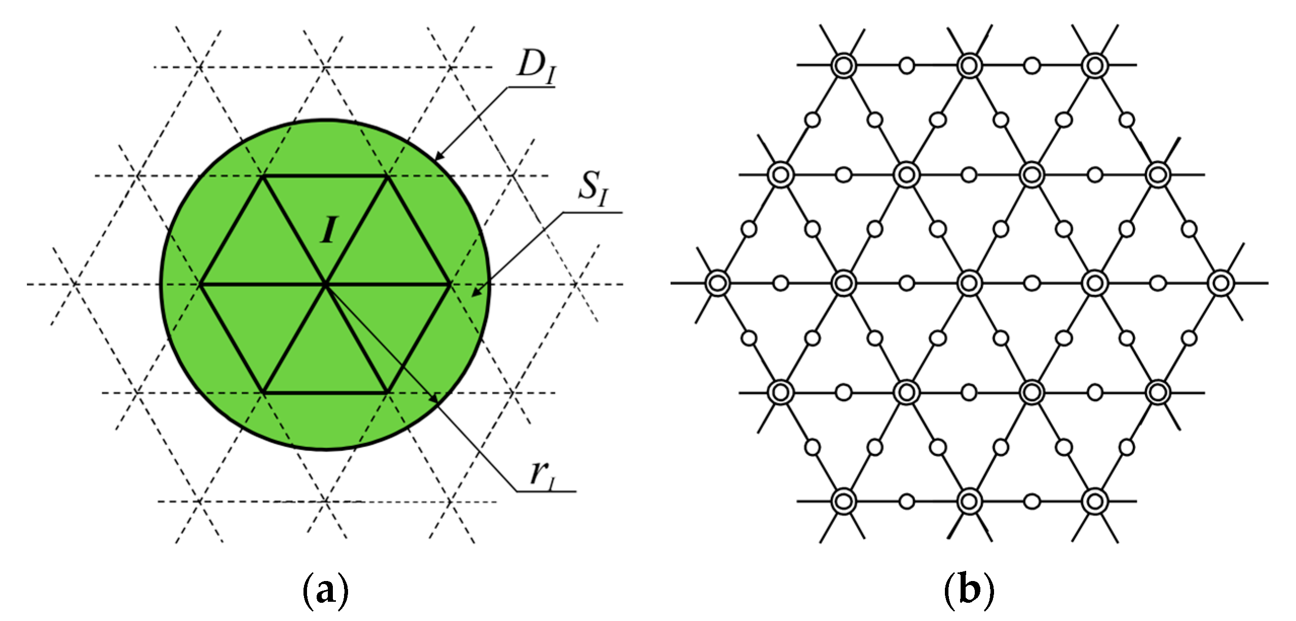
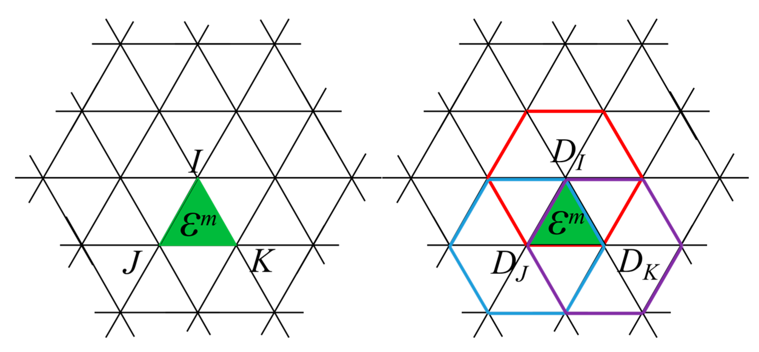
2. The Formulation of Overlapping Elements

The OFEM is a novel method that combines the advantages of the FEM and the mesh-free method. The main difference between the OFEM and the FEM lies in the construction of the local field approximation. In the traditional FEM, the nodal unknown is only a single value, while in the OFEM, the nodal unknown can be any reasonable function. In the OFEM, virtual nodes are utilized to form the partition of unity functions in the approximation of the local field while no degrees of freedom are given to these virtual nodes, which suppresses the linear dependence issue in some other generalized finite element methods. Moreover, the user-defined enrichment functions can be flexibly utilized in the local field, and thus, the numerical dispersions can be significantly mitigated. Then, the unknown coefficients turn to the amplitude of the enrichment functions rather than the nodal pressures.

2.1. Local Interpolation

As shown in Figure 1, the relevant variables of the local field are first defined. The local field DI of the node I consists of six triangular elements. Let N I be the set of nodes contained in DI and SI be the sphere including all nodes in DI. rI is the radius of the sphere SI. The approximations of the local field in the domain SI can be given by [46]
ψ I ( x ) = J N I n φ J I ( x ) ( p n α J n )
in which φ J I ( x ) is the interpolation function satisfying the PU, α J n denotes the unknown nodal field variables, and pn denotes the user-defined functions. Actually, any reasonable functions can be used in the OFEM, and in this work we mainly focus on complete polynomials of order n, with considerable generality in engineering practice
p = [ 1   x   y   x 2   x y   y 2   ]
where the variables (x, y) are measured from node J.
Then, in the new OFEM scheme shown in Figure 1, virtual nodes are automatically generated in each triangular element to construct the approximation of the local field. It is worth mentioning that the interpolation function φ J I ( x ) plays a significant role in dealing with mesh distortion. In the past scheme, the Shepard function is directly used in the overlapping formulation. In the new scheme, the interpolation function in every overlapping region is given as [46]
φ J I = i = 1 6 h ^ i φ ^ J i I
where h ^ i is the second-order shape function of the traditional FEM, and φ ^ J i I is the predefined weight function [46].

2.2. Global Interpolation

Once the approximation of the local field is obtained in the OFEM, the global approximation can be established by using the partition of unity. Consider a two-dimensional domain Ω, shown in Figure 2, is composed of Ne triangular elements and Nn nodes. In traditional FEM, the field variables in each element can be obtained by
u = h I u I
where hI (with I = i, j, k) is the shape function of the corresponding nodes and uI is the nodal field variable.
For the OFEM, the triangular domain ε m is the overlap region of the local domains DI, DJ, and DK. Im is the set of nodes which are the intersection of the local domain DI and the overlap region ε m . The global approximation in the present OFEM scheme is constructed as [46]
u ( x ) = m = 1 N e I I m h I ψ I ( x )
Substituting Equation (1) into Equation (5),
u ( x ) = m = 1 N e I I m h I J N I n φ J I ( x ) ( p n α J n )
The expression in Equation (6) can be rewritten as
u = J = 1 3 f J n p n α J n
with the new interpolation functions f J given as
f J = I = 1 3 h I φ ^ J I
Substituting the detailed expression of the weight function φ ^ J I into Equation (8), the interpolation function f J can be written as
f 1 = h ^ 1 + h ^ 4 ( h 1 + h 2 ) W 1 W 1 + W 2 x 4 + h ^ 4 h 3 W 1 W 1 + W 2 + W 3 x 4             + h ^ 5 h 1 W 1 W 1 + W 2 + W 3 x 5 + h ^ 6 ( h 1 + h 3 ) W 1 W 1 + W 3 x 6             + h ^ 6 h 2 W 1 W 1 + W 2 + W 3 x 6
f 2 = h ^ 2 + h ^ 4 ( h 1 + h 2 ) W 2 W 1 + W 2 x 4 + h ^ 4 h 3 W 2 W 1 + W 2 + W 3 x 4             + h ^ 5 ( h 2 + h 3 ) W 2 W 2 + W 3 x 5 + h ^ 5 h 1 W 2 W 1 + W 2 + W 3 x 5             + h ^ 6 h 2 W 2 W 1 + W 2 + W 3 x 6
f 3 = h ^ 3 + h ^ 4 h 3 W 3 W 1 + W 2 + W 3 x 4 + h ^ 5 ( h 2 + h 3 ) W 3 W 2 + W 3 x 5             + h ^ 5 h 1 W 3 W 1 + W 2 + W 3 x 5 + h ^ 6 ( h 1 + h 3 ) W 3 W 1 + W 3 x 6             + h ^ 6 h 2 W 3 W 1 + W 2 + W 3 x 6
in which the weight function W J ( J = 1 , 2 , 3 ) is defined as [41]
W J = 1 6 s 2 + 8 s 3 3 s 4           0 s 1 0                                                                       s > 1
with the variable s given by [46]
s = d J r J
where d J represents the distance from node J to point x = ( x , y ) .

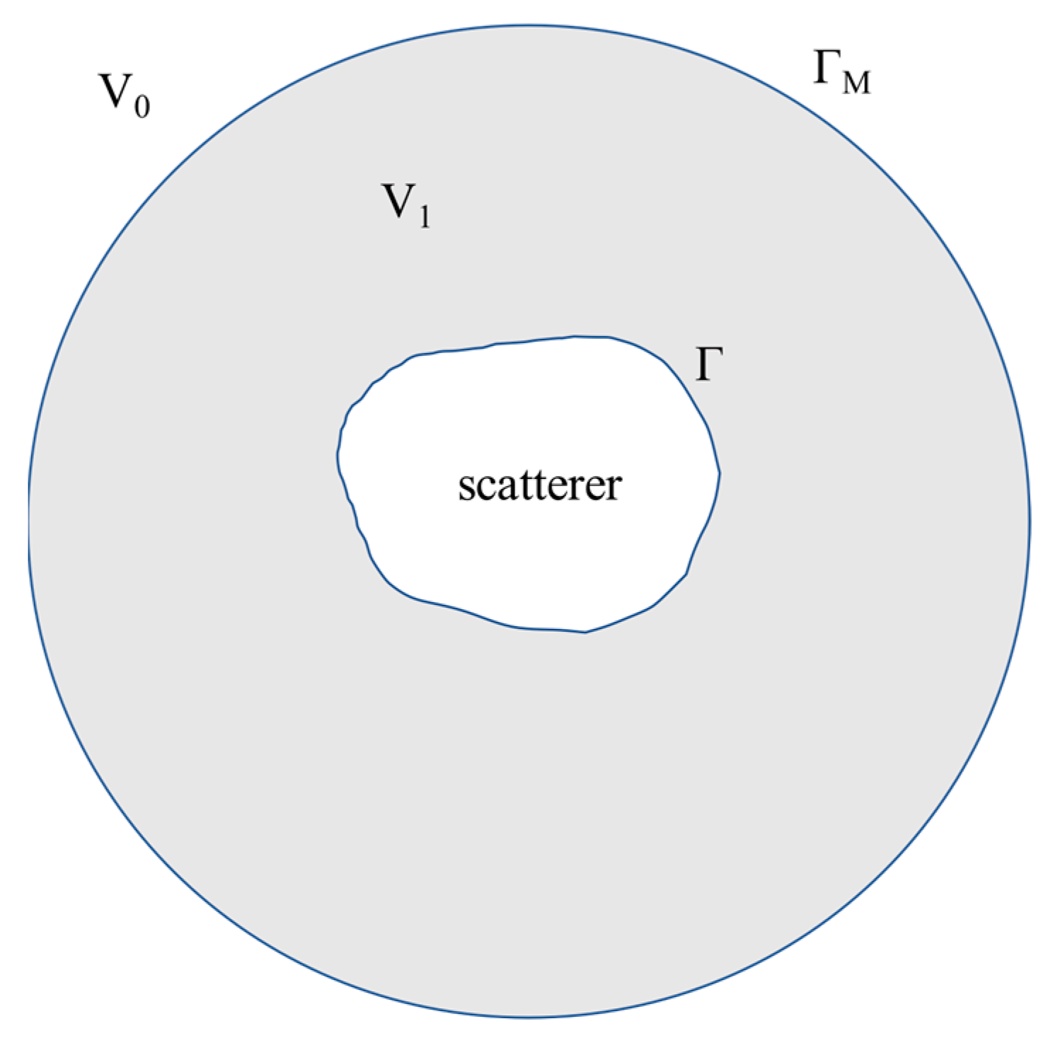
3. The Standard Galerkin Weak Form for the Exterior Acoustics

Considering a bounded problem domain Ω without an external source term, the acoustic medium inside this domain is homogeneous and inviscid. The boundary condition Γ consists of three parts, which are the Dirichlet boundary Γ D , the Neumann boundary Γ N , and the Robin boundary Γ R . Note that Γ D Γ N Γ R = Γ and Γ D Γ N Γ R = .
The acoustic pressure u can be obtained by solving the Helmholtz equation
2 u + k 2 u = 0
where is the Hamiltonian operator, k = ω / c is the wavenumber, and ω and c denote the angular frequency and wave speed, respectively.
The boundary conditions can be given as
u = u D     on   Γ D u · n = j ρ ω v n     on   Γ N u · n = j ρ ω A n u     on   Γ R
where n, ρ , A n represent the unit normal outwards vector on the boundary, the density of the media, and the admittance coefficient on the boundary Γ R , and v n is the normal velocity on the boundary Γ N .
In addition, according to the conservation of momentum, the acoustic particle velocity v can be related to the acoustic pressure u in the form of
u = j ρ ω v
By resorting to Equations (14) and (15), the acoustic field for interior acoustic problems can be easily sloved. However, for underwater acoustic scattering problems with an infinite problem domain, an artificial boundary is usually required to form the computational domain. Furthermore, the absorbing boundary conditions can be prescribed on this boundary to satisfy the Sommerfeld radiation condition
lim r r ( d 1 ) 2 u r j k u = 0
where d is the dimension of the considered problem.
There are many absorbing boundary conditions such as the DtN boundary condition [50], a family of Bayliss–Gunzburger–Turkel boundary conditions [58], and the perfectly matched layer technique [49,59]. Among these techniques, the DtN boundary condition is an exact non-reflection boundary condition without any additional manually selected parameters, and thus, is employed in this work. The shape of the DtN boundary is usually a circle, as shown in Figure 3. The exact acoustic pressure on Γ M is denoted as [49]
u ( r , θ ) = 1 π n = 0 0 2 π c n H n ( 1 ) ( k r ) H n ( 1 ) ( k R a ) cos   n ( θ ϑ ) u ( R a , ϑ ) d ϑ
where Ra is the radius of the DtN boundary; H n ( 1 ) is the Hankel function of the first kind; and
c n = 0.5 ,     n = 0 1 ,           n > 0
Taking the derivative of u with respect to argument r, the new equation is
u ( r , θ ) n r = R a = n = 0 c n 0 2 π m n ( θ ϑ ) u ( R a , ϑ ) d ϑ
in which
m n ( θ ϑ ) = k π H n ( 1 ) ( k R a ) H n ( 1 ) ( k R a ) cos n ( θ ϑ )
Equation (20) can be rewritten as
u ( r , θ ) n r = R a = M u ( R a , θ )
with M being the DtN operator, which makes the Sommerfeld radiation condition a boundary condition on the artificial boundary.
However, the infinite series involved in the DtN operator needs to be truncated in practical numerical implementation
u ( r , θ ) n r = R a n = 0 N c n 0 2 π m n ( θ ϑ ) u ( R a , ϑ ) d ϑ = M N u ( R a , θ )
where N is the number of truncated terms, and MN is the truncated DtN operator.
The number of truncated terms can affect the accuracy of the DtN boundary condition and the well-posedness regarding the uniqueness of solutions. To overcome these difficulties, a local differential operator B is applied in the modified DtN boundary condition. Assume B is a linear operator such that Equations (14) and (15) and u ( r , θ ) n r = R a = B u ( r , θ ) is a well-posed problem. The operator B is applied to the higher modes without modifying the exact boundary condition on the lower modes. Adding and subtracting operator B on the right side of Equation (23), the new equation is
u ( r , θ ) n r = R a M m N u ( R a , θ ) = M N B N u ( R a , θ ) B u ( R a , θ )
where M m N is the modified DtN operator.
However, it is necessary to present a suitable condition on B on higher modes. Detailed discussions about the operator B can be found in ref. [60]. In this work, the local differential operator is
B u ( r , θ ) r = R a = ( j k 1 2 R a ) u ( R a , θ )
Thus, the modified DtN boundary condition can be expressed as
u ( r , θ ) r r = R a = n = 0 N c n γ 0 2 π cos ( θ ϑ ) u ( R a , ϑ ) d ϑ ( j k 1 2 R a ) u ( R a , θ )
γ = 1 π ( k H n ( 1 ) ( k R a ) H n ( 1 ) ( k R a ) j k + 1 2 R a )
Then, the weak form of the exterior acoustic scattering problems can be constructed by resorting to the weighted residual method. Multiplying the weight function w on both sides of the Helmholtz equation and integrating over the problem domain Ω, the following equation can be reached
Ω w ( Δ u + k 2 u ) d Ω = 0
Integrating Equation (28) by parts, the new equation is
Ω w · u d Ω k 2 Ω w · u d Ω Γ w · ( u · n ) d Γ = 0
Applying the boundary conditions mentioned above, Equation (29) can be written as
Ω w · u d Ω k 2 Ω w · u d Ω + j ρ ω Γ N w · v n d Γ + j ρ ω A n Γ R w · u d Γ + Γ M w · M m N · u d Γ = 0
In the Galerkin form, the weight function is
w ( x ) = δ u ( x ) = i = 1 N n N i ( x ) δ u i = N ( x ) δ u
in which N i , u i are the shape function and the pressure value of the ith node, respectively.
Substitute Equation (31) into Equation (30), the new equation is
Ω ( N ) T · N d Ω U k w 2 Ω N T · N d Ω U + j ρ ω Γ R A n N T · N d Γ U + Γ M N T · M m N · N d Γ U = j ρ ω Γ N N T · v n d Γ
Equation (32) can be rewritten in the matrix form
( K k 2 M + j ρ ω C + K mDtN )   U = j ρ ω F
with:
the acoustic stiffness matrix K = Ω ( N ) T N d Ω ;
the acoustic mass matrix M = Ω N T N d Ω ;
the acoustic damping matrix C = Γ R A n N T N d Γ ;
the modified DtN matrix K mDtN = Γ M N T M m N N d Γ ;
the vector of acoustic force F = Γ N N T v n d Γ ;
the vector of unknown variables U = u 1 , u 2 , u 3 , , u n T .

4. Numerical Tests

In this section, the performance of OFEM in handling underwater acoustic scattering problems is investigated by several typical numerical examples. When the complete polynomials of the first and second order are used in the local basis functions in Equation (2), these schemes are termed as the OFEM-N3 and the OFEM-N6, respectively. In addition, the numerical results obtained by the traditional finite element discretization using the linear and the quadratic triangular elements are also given for comparison, and these schemes are termed the FEM-T3 and FEM-T6, respectively. The surrounding medium is water. The density is ρ = 1000 kg/m3 and the wave speed in water is c = 1500 m/s.

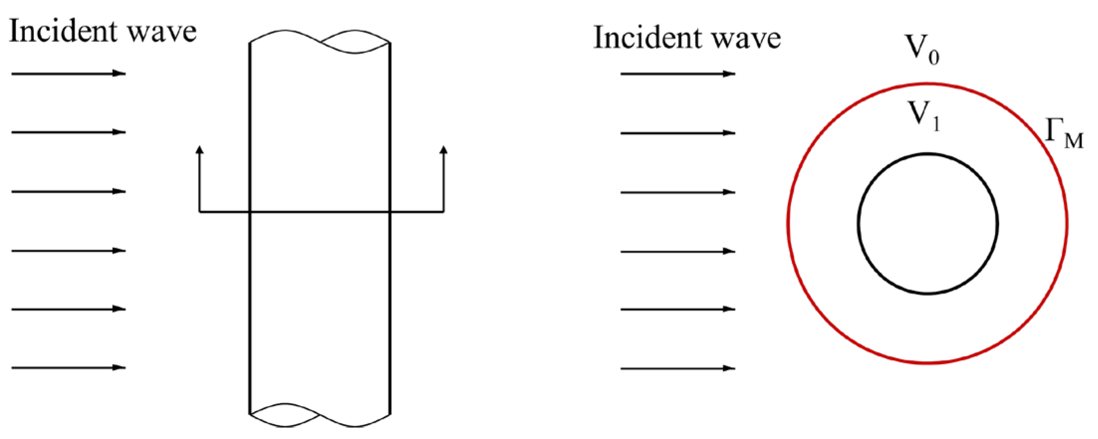
4.1. Cylinder Scattering in Underwater Acoustic Field

The acoustic scattering by an infinite rigid cylinder with radius a = 0.2 m is studied in this section. As shown in Figure 4, the incident wave is a unit plane wave and the direction of the wave is along the x-axis direction. Since variables are unchanged along the z-axis direction, this problem can be reduced to a two-dimensional problem. The DtN boundary is a circle centered at the origin with radius Ra = 1.2 m. Then, the acoustic scattering pressures can be sought by solving the following acoustic problem
Δ u + k w 2 u = 0       in   Ω u · n = j ρ ω v n     on   Γ N u ( R a , θ ) n = M m N u     on   Γ M
The analytical acoustic pressure can be obtained from
u = n = 0 + ( i ) n c n J n ( k a ) H n ( 1 ) ( k a ) H n ( 1 ) ( k r ) cos ( n θ )   ,
where J n and H n ( 1 ) are the Bessel function and Hankel function of the first kind, respectively.

4.1.1. The Computational Accuracy

The computational domain is discretized to be a set of triangular elements with the average element size h = 0.050 m as shown in Figure 5. In practical engineering projects, the rule of thumb [38], that more than six elements should be generated per wavelength, needs to be satisfied to generate an acceptable solution for the traditional finite element discretization.
The contour maps of acoustic pressure obtained from numerical methods and analytical solutions for k = 10 are displayed in Figure 6. It can be observed that the FEM-T3 yields almost meaningless results as apparent oscillations can be observed. In addition, by comparing the wavefront on which the acoustic pressure is 0.5 Pa, it is noted that the FEM-T6 and the OFEM-N3 can yield very similar solutions. Moreover, the numerical waves generated by these two schemes travel faster than the exact waves. This is because the numerical model of the two schemes has an over-stiff behavior [61,62], leading to a smaller numerical wavenumber than the exact wavenumber. By contrast, the OFEM-N6 model, with the close-to-exact stiffness of the exterior acoustic scattering systems, can provide the most precise solutions among all numerical methods.
Then, the real part of the scattering pressure at r = 1 m away from the center (the directivity patterns) for different wavenumbers is given in Figure 7 for detailed comparison. A similar conclusion can still be reached according to Figure 7. The solutions obtained from all of the numerical methods are consistent with the analytical results for the wavenumber k = 5, indicating that all of the numerical methods can achieve high accuracy at relatively low frequency. However, the solutions obtained from FEM-T3 are different from the analytical solutions for k = 10, 20, and 30. The curves of FEM-T6 and OFEM-N3 coincide with analytical solutions for wavenumbers k = 10 and k = 20, whereas apparent deviations can be noted between FEM-T6, OFEM-N3, and the analytical solution for wavenumber k = 30. By contrast, only OFEM-N6 can reach a high accuracy at the relatively high frequency.
To further measure the numerical solution accuracy, the following relative error indicator is adopted
γ e = Ω ( u exact u h ) T ( u exact u h ) d Ω Ω u exact T u exact d Ω
where u* is the complex conjugate of the pressure u, and the superscripts ‘exact’ and ‘h’ represent the analytical solutions and the numerical solutions, respectively.
Figure 8 illustrates the relationship between the relative error and the wavenumber. It can be observed that the relative error of all of the numerical methods rises with increasing wavenumber in the acoustic scattering problems. The FEM-T6 behaves in a similar way to the OFEM-N3 and can provide a reasonable solution accuracy for non-dimensional wavenumber kh < 1. In addition, the relative error in OFEM-N6 increases slowly and is less than 1% for all computed wavenumbers. Note that the overlapping elements can be applied to the finite element model without changing the mesh topology. This means that the p-adaptive analysis can be easily achieved and the available computational frequency range of the original numerical model can be enlarged flexibly.

4.1.2. The Control of the Numerical Error

The performance of all schemes in the acoustic scattering problem deteriorates with increasing wavenumber, indicating that the numerical pollution effect is also inevitable in high-order elements. Actually, the total numerical errors in H1 semi-norm in the traditional FEM have been studied and can be bounded by [63]
γ H C 1 ( k h n ) n + C 2 k ( k h n ) 2 n
where C1 and C2 are constant coefficients which are unrelated to the wavenumber k and the average element size h; n represents the order of the shape functions.
In Equation (37), the dispersive error is the first term and the second term is the interpolation error. When the wavenumber k is kept to a small value, both the interpolation error and the dispersive error are maintained at a reasonable level. However, for a large computational frequency, the total numerical errors can surge sharply. This means that another effective criterion instead of the rule of thumb is required for the control of the total numerical error.
To further investigate the criterion for controlling numerical errors, two schemes are compared separately. First, keeping the non-dimensional wavenumber kh as a constant to control the interpolation error as the requirement of the rule of thumb. Second, keeping the term k3h2 as a constant to control the dispersion error. The results of the above two cases are displayed in Figure 9. There is an obvious rise in the relative errors of the traditional FEM as the average element size decreases when kh is constant. The same conclusion can be obtained for OFEM-N3. It is interesting to note in the OFEM-N6 scheme that there is a turning point at the average element size h = 0.0295 m. With a larger element size, the relative error can be well controlled with the mesh refinement, but with a smaller size, the solution accuracy deteriorates with the mesh refinement.
As for the second criterion, where the term k3h2 is kept as a constant, the solution accuracy of all methods can be improved with decreasing the element size. Moreover, the convergence rate of the OFEM-N6 is higher than that of the OFEM-N3, and the OFEM-N6 can always yield the most accurate solutions. Considering that the high-order elements are easily reached without any mesh adjustment, the coupled OFEM model possesses significantly superior in controlling the total numerical errors in underwater acoustic problems.

4.1.3. The Convergence Property

As shown in Figure 10, the convergence of all of the schemes is studied with k = 20. It can be observed that the numerical errors go down with the mesh refinement, revealing that all numerical methods are convergent. Moreover, the solution accuracy of the OFEM-N3 and the FEM-T6 is almost identical for the relatively small non-dimensional wavenumber kh. In addition, the OFEM-N6 can yield very satisfactory solutions even by using a very coarse mesh, indicating that the coupled OFEM is very promising in handling underwater acoustic scattering problems.

4.1.4. Sensitivity to Nodal Irregularity

A comparison of different methods between regular meshes and irregular meshes is made to assess the influence of a distorted mesh on the solution accuracy. The irregular meshes are generated based on the regular meshes
x = x + Δ x · r c · β i r y = y + Δ y · r c · β i r
where x′ and y′ are the coordinates of the irregular nodes, x and y are the coordinates of the regular nodes, Δx and Δy are the regular nodal spacings in the x-axis and y-axis directions, r c is a random number whose value is between −1 and 1, and β i r is a prescribed parameter that can control the irregularity degree.
The directivity patterns at different wavenumbers are plotted in Figure 11. A precise solution can be provided by four numerical methods at a low frequency using irregular meshes. As Figure 11 shows for wavenumber k = 10, the conventional FEM is sensitive to irregular meshes. There is a slight difference between the analytical solution and the solution of OFEM at wavenumber k = 25. Moreover, the solution of OFEM-N6 is consistent with the analytical solution all the time.
Further studies were performed in the sensitivity analysis. The result of the OFEM with an irregular mesh is plotted in Figure 12. The result is fairly accurate even for wavenumber k = 40, which is twice the wavenumber obtained from the rule of thumb.

4.1.5. The Computational Efficiency

Figure 13 illustrates the relationship between the error, γn, and time, t. It is apparent that the performance of the traditional FEM-T3, regarding the computational efficiency, is undesirable because more computational time is needed to reach a comparable solution accuracy. However, the computational times of the FEM-T6 and the OFEM with linear and quadratic local basis functions are much more similar for a comparable solution accuracy. This phenomenon does not mean that the coupled OFEM is inferior to the traditional FEM using high-order elements in terms of the computational efficiency. We herein emphasize again that the high-order functions can be directly added into the approximation space because all of these enriched DOFs are only associated with the vertex nodes of each element, meaning that no mesh adjustment is needed, while in the traditional FEM, the efficiency of the hp-adaptive analysis is related to the mesh refinement strategy [64,65]. In addition, as mentioned before, any reasonable nodal DOFs can be included in the OFEM to further improve its performance, as in the GFEM/PUFEM, but the linear dependence issue can be avoided in the OFEM, while additional treatments are required [63,66] in the GFEM/PUFEM to handle the singular coefficient matrix when Lagrange polynomial functions are used in the approximations. Actually, for a similar computational accuracy, the OFEM-N6 requires the least number of elements to discretize the problem domain according to the convergence curve in Figure 13, meaning that the coupled OFEM can significantly reduce the cost in dividing an adequate mesh in the acoustic scattering problem.

4.2. Scattering by a Rudder-Shaped Scatterer

The scattering of a rudder is studied in this section. The geometry of the considered scatterer is obtained from the NACA0010 airfoil with length L = 1 m for simplification. The diameter of the DtN boundary is 4 m. The sketch map is shown in Figure 14.
The computational domain is bounded by the rubber and the DtN boundary with the average element size of h = 0.0628 m. The scattered acoustic pressure obtained from FEM-T6 with a small element size is considered as a reference.
The distributions of the real part of the acoustic pressure for wavenumber k = 5 and k = 20 are presented in Figure 15 and Figure 16, respectively. When the frequency is in a relatively lower range, the results computed from all numerical methods are consistent with the analytical solution. It is noted that the acoustic wave travels faster in FEM-T3 than the acoustic wave in the reference solution for wavenumber k = 20 because of the ‘overly stiff’ numerical model from the conventional FEM.

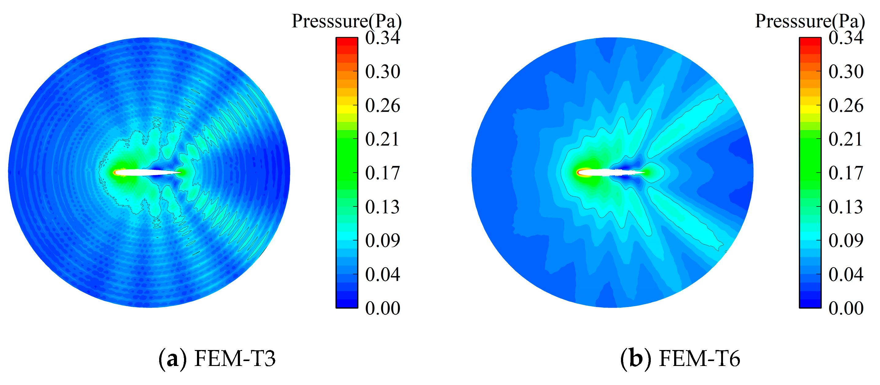
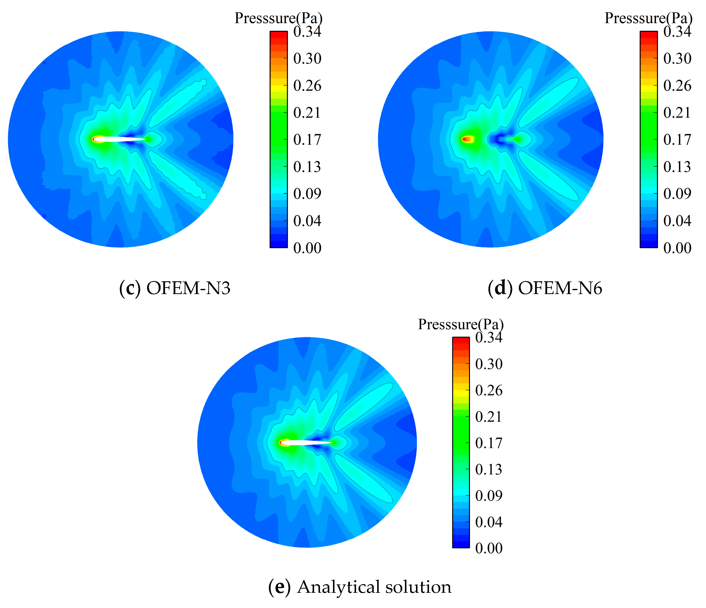
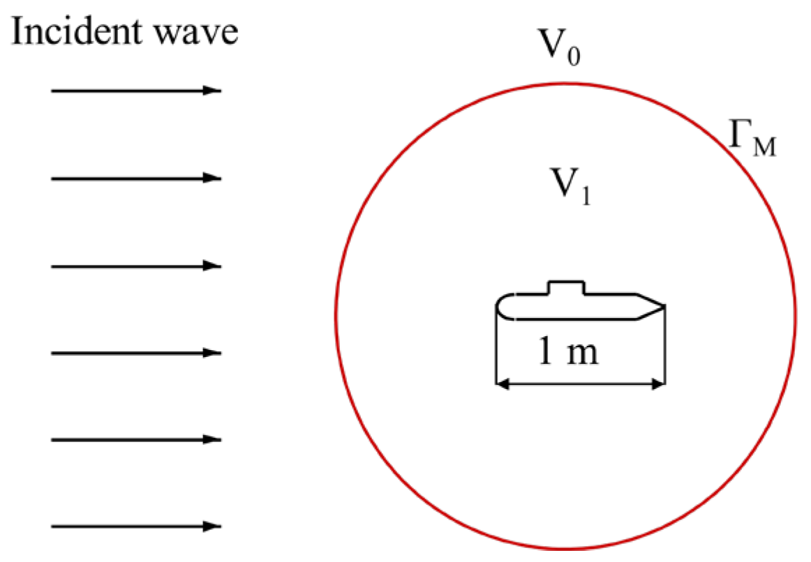
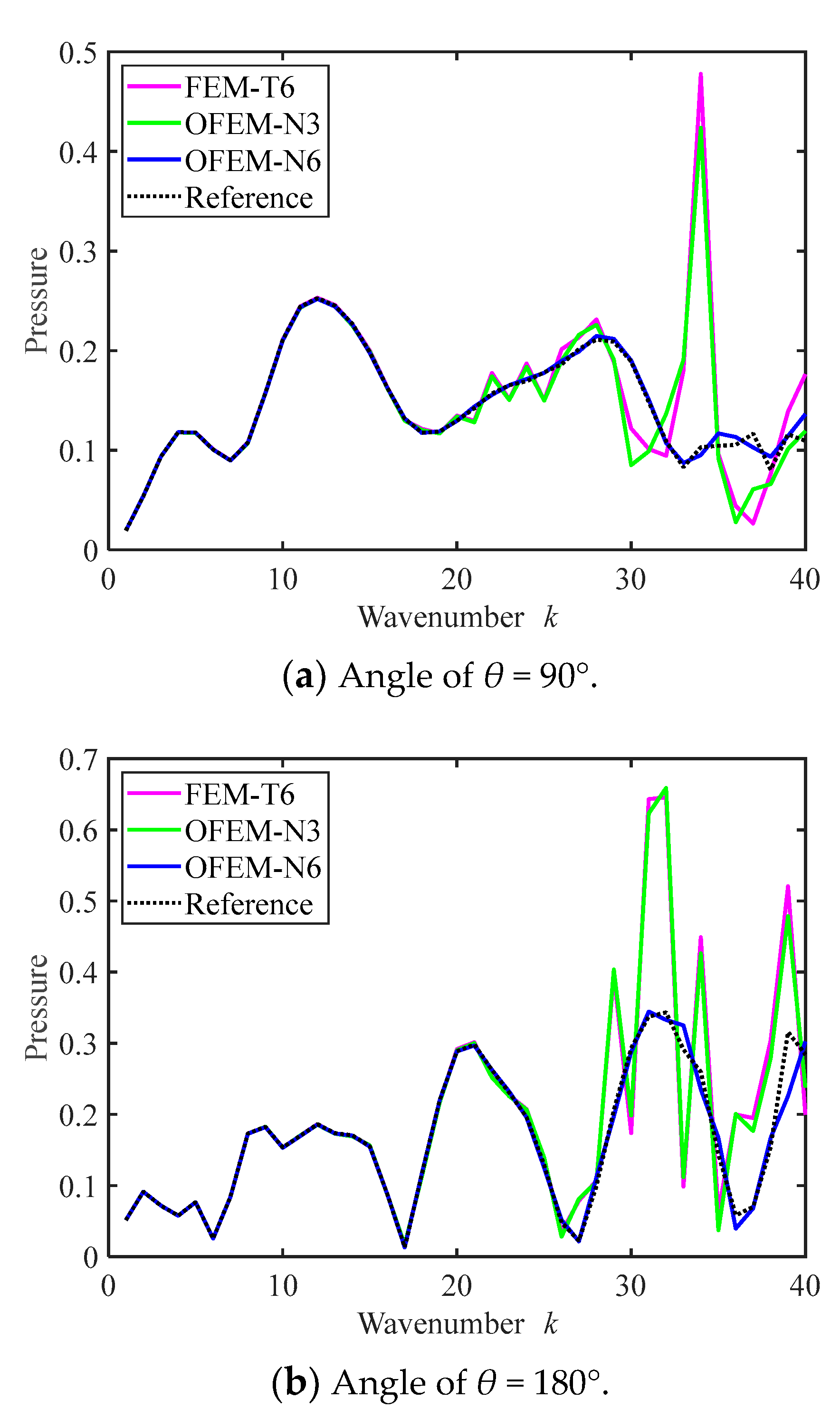
4.3. Scattering by a Submarine Scatterer

Consider an acoustic field where the acoustic wave is scattered by a submarine structure. This structure is normalized and the length is 1 m. The incident wave of the acoustic field is the plane simple harmonic wave which travels along the x-axis direction. The radius of the artificial boundary is 2 m. The sketch map is shown in Figure 17. There are two observation points at a distance of 1 m with angles θ = 90° and θ = 180°.
There is no available analytical solution for the acoustic scattering by a submarine scatterer, so a reference solution is obtained for the high-order FEM with finer meshes. The scattering problem is solved with different numerical methods for comparison. The results of the real part of pressure at the observation points are displayed in Figure 18. Figure 18 indicates that the numerical solution of the OFEM is in accord with the reference solution. The numerical solution of FEM-T6 is also fairly accurate. There is a certain deviation for the solution of FEM-T3 when the wavenumber is more than k = 18. The result of the observation at the angle θ = 180° shows a good performance of the OFEM.

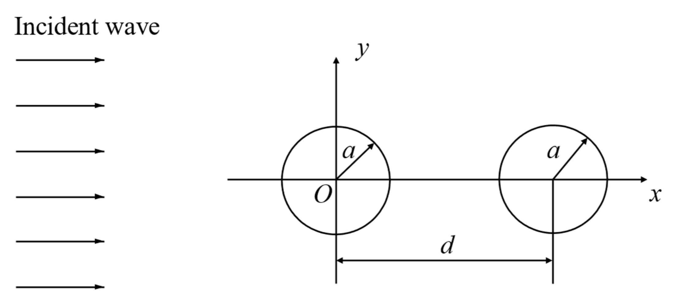
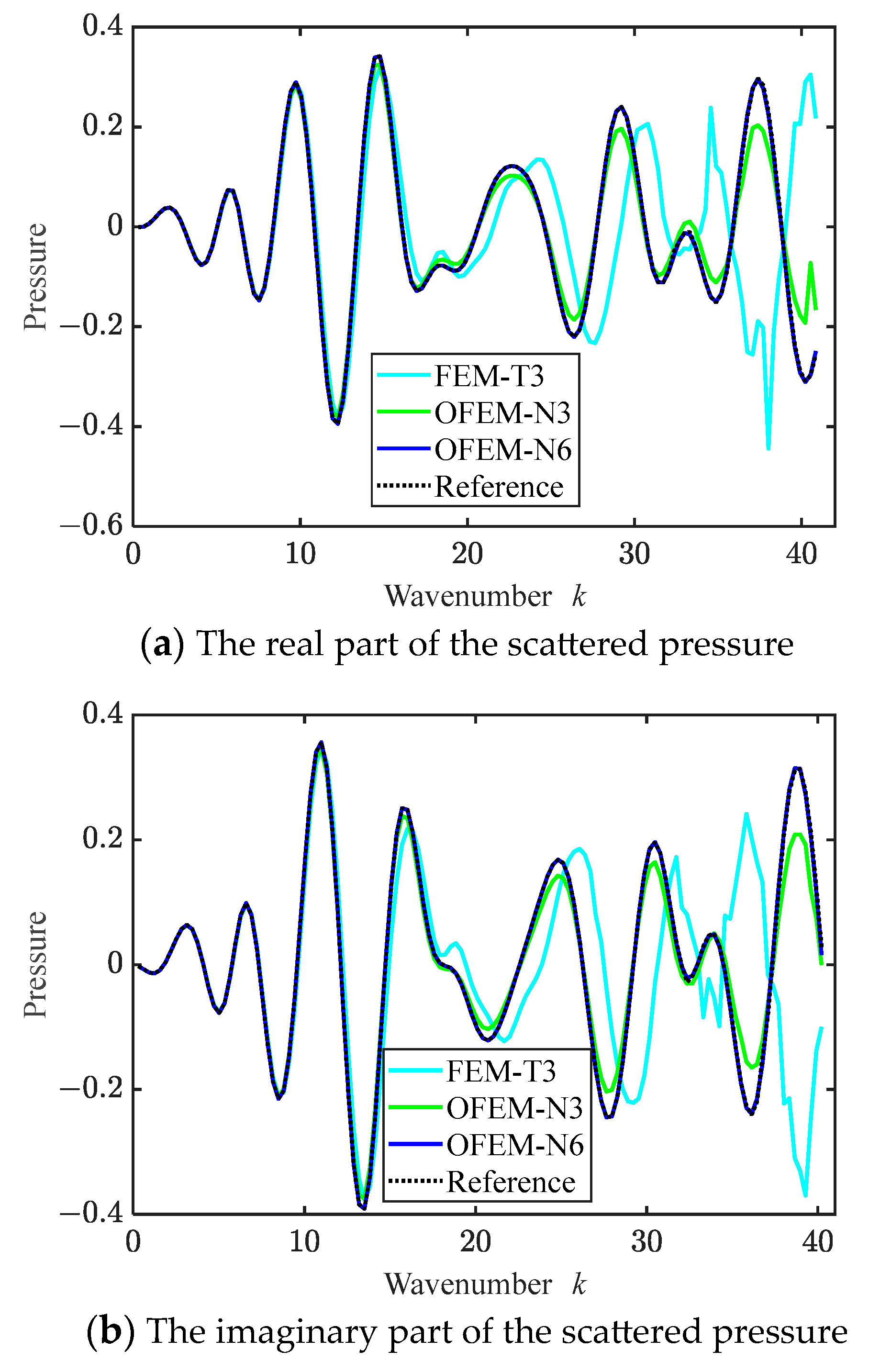
4.4. The Multi-Object Scattering Problem

The multi-object acoustic scattering problem is examined in the frequency domain to illustrate the performance of the OFEM in this section. As shown in Figure 19, the multi-object system consists of two cylinders with radii of a = 0.2 m. The centers of the cylinders are located at the origin and (0.4, 0), respectively. The cylinders are surrounded by water with a density of 1000 kg/m3. The infinite domain is truncated by an artificial boundary, which is a circle centered at the origin with a radius of 1.2 m. The incident wave travels in the x-axis direction with a speed of c = 1500 m/s. The observation points are located on a circle centered at the origin with a radius of 1 m in different directions. Since the system is complex and it is difficult to derive a theoretical solution, a reference solution is obtained from a high-order finite element analysis with a refined mesh.
Figure 20 illustrates the acoustic scattering pressure versus the wavenumber k with different numerical methods. According to the results of the previous example, the performance of the proposed OFEM-N3 is similar to that of the classic quadratic triangular finite element. Thus, the solutions of the conventional FEM-T6 are not plotted in Figure 20. It can be found that all solutions obtained from numerical methods are exact in the low frequency range. However, in the higher frequency range, there is a deviation between the solutions obtained from the FEM and the reference solutions, while the OFEM-N6 solutions are consistent with the reference solutions.

5. Conclusions

In this work, a coupled OFEM for solving underwater acoustic scattering problems is proposed by combining the overlapping element and the modified Dirichlet-to-Neumann boundary condition. Any reasonable nodal DOFs can be included in the OFEM to further improve its performance as in the GFEM/PUFEM, but the linear dependence issue can be avoided in the OFEM. By using the modified Dirichlet-to-Neumann boundary condition, better solution precision can be achieved than the original truncated form with fewer terms, and unique solutions can be ensured. According to the numerical tests, the following conclusions can be given.
The coupled OFEM shows better accuracy and stability in computing underwater scattering problems in an unbounded field compared to a conventional finite element method. Considering that the high-order elements can be easily reached without any mesh adjustment, the coupled OFEM model is significantly superior in controlling the total numerical errors. Therefore, the OFEM behaves well even with relatively high wavenumbers in the underwater acoustic problems. Moreover, the OFEM has better convergence properties, which means that a more accurate solution can be obtained with less computation. In addition, the OFEM is much less sensitive to distorted meshes, meaning that the coupled OFEM can significantly reduce the cost of dividing an adequate mesh in the acoustic scattering problem. The superiority of the coupled OFEM is that p-adaptive analysis can be easily achieved to improve the solution accuracy without the linear dependence problem of the classic GFEM/PUFEM.
However, additional degrees of freedom (DOFs) are associated with each field node, and thus, the total number of DOFs still increase with the increasing computational frequencies in practical engineering scenarios, which limits the application of the coupled OFEM for acoustic problems at relatively high frequencies due to the finite computing resource. Future studies may mitigate this issue further by using a model order reduction technique or efficient adaptive analysis strategy.

Author Contributions

B.J.: conceptualization, methodology, validation, formal analysis, writing—original draft, writing—review and editing. J.Y.: conceptualization, methodology, formal analysis, writing—review and editing, supervision. W.L.: conceptualization, methodology, formal analysis, writing—review and editing, supervision. Y.C.: conceptualization, methodology, formal analysis, writing—review and editing, supervision. Q.G.: conceptualization, methodology, validation, formal analysis, writing—review and editing. All authors have read and agreed to the published version of the manuscript.

Funding

This research was funded by the National Natural Science Foundation of China (Contract No. 52171336 and No. 12202327), and Hubei Province Natural Science Foundation (Grant No. 2021CFB028).

Data Availability Statement

The data used in this work will be made available on request.

Conflicts of Interest

The authors declare no conflict of interest.

References

  1. Gong, Z.X.; Li, W.; Chai, Y.B.; Zhao, Y.; Mitri, F.G. T-matrix method for acoustical Bessel beam scattering from a rigid finite cylinder with spheroidal endcaps. Ocean Eng. 2017, 129, 507–519. [Google Scholar] [CrossRef]
  2. Zheng, Z.Y.; Li, X.L. Theoretical analysis of the generalized finite difference method. Comput. Math. Appl. 2022, 120, 1–14. [Google Scholar] [CrossRef]
  3. Zhang, Y.; Yang, Y.Z.; Chai, Y.B.; Li, W. Graphical acoustic computing method incorporated with the shooting and bouncing ray: Application to target strength prediction of concave objects with second-order reflection effects. J. Sound Vibr. 2022, 541, 117358. [Google Scholar] [CrossRef]
  4. Fu, Z.J.; Xie, Z.Y.; Ji, S.Y.; Tsai, C.C.; Li, A.L. Meshless generalized finite difference method for water wave interactions with multiple-bottom-seatedcylinder-array structures. Ocean. Eng. 2022, 195, 106736. [Google Scholar] [CrossRef]
  5. Li, Y.C.; Dang, S.N.; Li, W.; Chai, Y.B. Free and Forced Vibration Analysis of Two-Dimensional Linear Elastic Solids Using the Finite Element Methods Enriched by Interpolation Cover Functions. Mathematics 2022, 10, 456. [Google Scholar] [CrossRef]
  6. He, Z.C.; Hu, J.Y.; Li, E. An uncertainty model of acoustic metamaterials with random parameters. Comput. Mech. 2018, 62, 1023–1036. [Google Scholar] [CrossRef]
  7. He, Z.C.; Lin, X.Y.; Li, E. A non-contact acoustic pressure-based method for load identification in acoustic-structural interaction system with non-probabilistic uncertainty. Appl. Acoust. 2019, 148, 223–237. [Google Scholar] [CrossRef]
  8. Li, E.; He, Z.C.; Wang, G.; Liu, G.R. An efficient algorithm to analyze wave propagation in fluid/solid and solid/fluid phononic crystals. Comput. Methods Appl. Mech. Eng. 2018, 333, 421–442. [Google Scholar] [CrossRef]
  9. Li, J.P.; Fu, Z.J.; Gu, Y.; Zhang, L. Rapid calculation of large-scale acoustic scattering from complex targets by a dual-level fast direct solver. Comput. Math. Appl. 2023, 130, 1–9. [Google Scholar] [CrossRef]
  10. Li, J.P.; Fu, Z.J.; Gu, Y.; Zhang, L. Recent advances and emerging applications of the singular boundary method for large-scale and high-frequency computational acoustics. Adv. Appl. Math. Mech. 2022, 14, 315–343. [Google Scholar] [CrossRef]
  11. Simpson, R.N.; Bordas, S.P.; Lian, H.; Trevelyan, J. An isogeometric boundary element method for elastostatic analysis: 2D implementation aspects. Comput. Struct. 2013, 118, 2–12. [Google Scholar] [CrossRef]
  12. Qiu, T. Time Domain Boundary Integral Equation Methods in Acoustics, Heat Diffusion and Electromagnetism. Ph.D. Thesis, University of Delaware, Newark, DE, USA, 2016. [Google Scholar]
  13. Kirkup, S. The Boundary Element Method in Acoustics: A Survey. Appl. Sci. 2019, 9, 1642. [Google Scholar] [CrossRef]
  14. Gu, Y.; Lei, J. Fracture mechanics analysis of two-dimensional cracked thin structures (from micro- to nano-scales) by an efficient boundary element analysis. Results Appl. Math. 2021, 11, 100172. [Google Scholar] [CrossRef]
  15. Liu, Y.J. Fast Multipole Boundary Element Method: Theory and Applications in Engineering; Cambridge University Press: Cambridge, UK, 2009. [Google Scholar]
  16. Ayala, T.; Videla, J.; Anitescu, C.; Atroshchenko, E. Enriched Isogeometric Collocation for two-dimensional time-harmonic acoustics. Comput. Methods Appl. Mech. Eng. 2020, 365, 113033. [Google Scholar] [CrossRef]
  17. Sun, T.T.; Wang, P.; Zhang, G.J.; Chai, Y.B. Transient analyses of wave propagations in nonhomogeneous media employing the novel finite element method with the appropriate enrichment function. Comput. Math. Appl. 2023, 139, 90–112. [Google Scholar] [CrossRef]
  18. Chai, Y.B.; Huang, K.Y.; Wang, S.P.; Xiang, Z.C.; Zhang, G.J. The Extrinsic Enriched Finite Element Method with Appropriate Enrichment Functions for the Helmholtz Equation. Mathematics 2023, 11, 1664. [Google Scholar] [CrossRef]
  19. Ihlenburg, F.; Babuška, I. Finite element solution of the Helmholtz equation with high wave number Part I: The h-version of the FEM. Comput. Math. Appl. 1995, 30, 9–37. [Google Scholar] [CrossRef]
  20. Ihlenburg, F.; Babuška, I. Finite element solution of the Helmholtz equation with high wave number part II: The hp version of the FEM. SIAM J. Numer. Anal. 1997, 34, 315–358. [Google Scholar] [CrossRef]
  21. Liu, G.R.; Trung, N.T. Smoothed Finite Element Methods; CRC Press: Boca Raton, FL, USA, 2010. [Google Scholar]
  22. Zeng, W.; Liu, G.R. Smoothed Finite Element Methods (S-FEM): An Overview and Recent Developments. Arch. Computat. Methods Eng. 2018, 25, 397–435. [Google Scholar] [CrossRef]
  23. Chai, Y.B.; Li, W.; Liu, Z.Y. Analysis of transient wave propagation dynamics using the enriched finite element method with interpolation cover functions. Appl. Math. Comput. 2022, 412, 126564. [Google Scholar] [CrossRef]
  24. Li, W.; Gong, Z.X.; Chai, Y.B.; Cheng, C.; Li, T.Y.; Zhang, Q.F.; Wang, M.S. Hybrid gradient smoothing technique with discrete shear gap method for shell structures. Comput. Math. Appl. 2017, 74, 1826–1855. [Google Scholar] [CrossRef]
  25. Chai, Y.B.; Li, W.; Gong, Z.X.; Li, T.Y. Hybrid smoothed finite element method for two-dimensional underwater acoustic scattering problems. Ocean Eng. 2016, 116, 129–141. [Google Scholar] [CrossRef]
  26. Melenk, J.M.; Babuška, I. The partition of unity finite element method: Basic theory and applications. Comput. Methods Appl. Mech. Eng. 1996, 139, 289–314. [Google Scholar] [CrossRef]
  27. Babuška, I.; Melenk, J.M. The partition of unity method. Int. J. Numer. Methods Eng. 1997, 40, 727–758. [Google Scholar] [CrossRef]
  28. Duarte, C.A.; Babuška, I.; Oden, J.T. Generalized finite element methods for three-dimensional structural mechanics problems. Comput. Struct. 1999, 77, 215–232. [Google Scholar] [CrossRef]
  29. Liu, G.R.; Gu, Y.T. An Introduction to Meshfree Methods and Their Programming; Springer Science & Business Media: Boston, NY, USA, 2005. [Google Scholar]
  30. Gu, Y.T.; Wang, W.; Zhang, L.C.; Feng, X.Q. An enriched radial point interpolation method (e-RPIM) for analysis of crack tip fields. Eng. Fract. Mech. 2011, 78, 175–190. [Google Scholar] [CrossRef]
  31. Belytschko, T.; Lu, Y.Y.; Gu, L. Crack propagation by element-free Galerkin methods. Eng. Fract. Mech. 1995, 51, 295–315. [Google Scholar] [CrossRef]
  32. Bouillard, P.; Suleaub, S. Element-Free Galerkin solutions for Helmholtz problems: Fomulation and numerical assessment of the pollution effect. Comput. Methods Appl. Mech. Eng. 1998, 162, 317–335. [Google Scholar] [CrossRef]
  33. Li, Y.C.; Liu, C.; Li, W.; Chai, Y.B. Numerical investigation of the element-free Galerkin method (EFGM) with appropriate temporal discretization techniques for transient wave propagation problems. Appl. Math. Comput. 2023, 442, 127755. [Google Scholar] [CrossRef]
  34. Liu, W.K.; Jun, S.; Zhang, Y.F. Reproducing kernel particle methods. Int. J. Numer. Methods Fluids 1995, 20, 1081–1106. [Google Scholar] [CrossRef]
  35. Atluri, S.N.; Zhu, T. A new meshless local Petrov-Galerkin (MLPG) approach in computational mechanics. Comput. Mech. 1998, 22, 117–127. [Google Scholar] [CrossRef]
  36. Xu, Y.Y.; Zhang, G.Y.; Zhou, B.; Wang, H.Y.; Tang, Q. Analysis of acoustic radiation problems using the cell-based smoothed radial point interpolation method with Dirichlet-to-Neumann boundary condition. Eng. Anal. Bound. Elem. 2019, 108, 447–458. [Google Scholar] [CrossRef]
  37. Li, W.; Zhang, Q.F.; Gui, Q.; Chai, Y.B. A coupled FE-Meshfree triangular element for acoustic radiation problems. Int. J. Comput. Methods. 2021, 18, 2041002. [Google Scholar] [CrossRef]
  38. You, X.Y.; Li, W.; Chai, Y.B. Dispersion analysis for acoustic problems using the point interpolation method. Eng. Anal. Bound. Elem. 2018, 94, 79–93. [Google Scholar] [CrossRef]
  39. You, X.Y.; Gui, Q.; Zhang, Q.F.; Chai, Y.B.; Li, W. Meshfree simulations of acoustic problems by a radial point interpolation method. Ocean Eng. 2020, 218, 108202. [Google Scholar] [CrossRef]
  40. You, X.Y.; Li, W.; Chai, Y.B.; Yu, Y. Numerical investigations of edge-based smoothed radial point interpolation method for transient wave propagations. Ocean Eng. 2022, 266, 112741. [Google Scholar] [CrossRef]
  41. Liu, C.; Min, S.; Pang, Y.; Chai, Y. The Meshfree Radial Point Interpolation Method (RPIM) for Wave Propagation Dynamics in Non-Homogeneous Media. Mathematics 2023, 11, 523. [Google Scholar] [CrossRef]
  42. De, S.; Bathe, K.J. The method of finite spheres. Comput. Mech. 2000, 25, 329–345. [Google Scholar] [CrossRef]
  43. De, S.; Bathe, K.J. The method of finite spheres with improved numerical integration. Comput. Struct. 2001, 79, 2183–2196. [Google Scholar] [CrossRef]
  44. Bathe, K.J.; Zhang, L.B. The finite element method with overlapping elements—A new paradigm for CAD driven simulations. Comput. Struct. 2017, 182, 526–539. [Google Scholar] [CrossRef]
  45. Zhang, L.B.; Bathe, K.J. Overlapping finite elements for a new paradigm of solution. Comput. Struct. 2017, 187, 64–76. [Google Scholar] [CrossRef]
  46. Zhang, L.B.; Kim, K.T.; Bathe, K.J. The new paradigm of finite element solutions with overlapping elements in CAD–Computational efficiency of the procedure. Comput. Struct. 2018, 199, 1–17. [Google Scholar] [CrossRef]
  47. Gui, Q.; Li, W.; Chai, Y.B. The enriched quadrilateral overlapping finite elements for time-harmonic acoustics. Appl. Math. Comput. 2023, 451, 128018. [Google Scholar] [CrossRef]
  48. Bathe, K.J. Finite element method. In Wiley Encyclopedia of Computer Science and Engineering; John Wiley & Sons, Inc.: New York, NY, USA, 2007; pp. 1–12. [Google Scholar]
  49. Xu, J.Q.; Hu, H.S.; Liu, Q.H.; Han, B.; Berenger, J.P. A high-order perfectly matched layer scheme for second-order spectral-element time-domain elastic wave modelling. J. Comput. Phys. 2023, 491, 112373. [Google Scholar] [CrossRef]
  50. Grote, M.J.; Keller, J.B. On nonreflecting boundary conditions. J. Comput. Phys. 1995, 122, 231–243. [Google Scholar] [CrossRef]
  51. Wu, S.W.; Xiang, Y. A weak-form meshfree coupled with infinite element method for predicting acoustic radiation. Eng. Anal. Bound. Elem. 2019, 107, 63–78. [Google Scholar] [CrossRef]
  52. Wu, S.W.; Xiang, Y.; Li, G.N. A coupled weak-form meshfree method for underwater noise prediction. Eng. Comput. 2022, 38, 5091–5109. [Google Scholar] [CrossRef]
  53. Merchant, N.D.; Blondel, P.; Dakin, D.T.; Dorocicz, J. Averaging underwater noise levels for environmental assessment of shipping. J. Acoust. Soc. Am. 2012, 132, EL343–EL349. [Google Scholar] [CrossRef]
  54. Kellett, P.; Turan, O.; Incecik, A. A study of numerical ship underwater noise prediction. Ocean Eng. 2013, 66, 113–120. [Google Scholar] [CrossRef]
  55. Alahmadi, H.; Afsar, H.; Nawaz, R.; Alkinidri, M.O. Scattering characteristics through multiple regions of the wave-bearing trifurcated waveguide. Waves Random Complex Media 2022, 1–17. [Google Scholar] [CrossRef]
  56. Nawaz, R.; Lawrie, J.B. Scattering of a fluid-structure coupled wave at a flanged junction between two flexible waveguides. J. Acoust. Soc. Am. 2013, 134, 1939–1949. [Google Scholar] [CrossRef]
  57. Nawaz, R.; Yaseen, A.; Alkinidri, M.O. Fluid–structure coupled response of dynamical surfaces tailored in a flexible shell. Math. Mech. Solids 2023. [Google Scholar] [CrossRef]
  58. Tezaur, R.; Macedo, A.; Farhat, C.; Djellouli, R. Three-dimensional finite element calculations in acoustic scattering using arbitrarily shaped convex artificial boundaries. Int. J. Numer. Methods Eng. 2002, 53, 1461–1476. [Google Scholar] [CrossRef]
  59. Harari, I.; Slavutin, M.; Turkel, E. Analytical and numerical studies of a finite element PML for the Helmholtz equation. J. Comput. Acoust. 2000, 8, 121–137. [Google Scholar] [CrossRef]
  60. Keller, J.B.; Givoli, D. Exact non-reflecting boundary conditions. J. Comput. Phys. 1989, 82, 172–192. [Google Scholar] [CrossRef]
  61. Li, E.; He, Z.C. Optimal balance between mass and smoothed stiffness in simulation of acoustic problems. Appl. Math. Model. 2019, 75, 1–22. [Google Scholar] [CrossRef]
  62. Wu, S.W.; Xiang, Y.; Li, W.Y. A hybrid smoothed moving least-squares interpolation method for acoustic scattering problems. Eng. Comput. 2023, 1–19. [Google Scholar] [CrossRef]
  63. Gui, Q.; Zhang, G.Y.; Chai, Y.B.; Li, W. A finite element method with cover functions for underwater acoustic propagation problems. Ocean Eng. 2022, 243, 110174. [Google Scholar] [CrossRef]
  64. Babuska, I.; Szabo, B.A.; Katz, I.N. The p-version of the finite element method. SIAM J. Numer. Anal. 1981, 18, 515–545. [Google Scholar] [CrossRef]
  65. Liu, W.K.; Li, S.; Park, H.S. Eighty Years of the Finite Element Method: Birth, Evolution, and Future. Arch. Comput. Method Eng. 2022, 29, 4431–4453. [Google Scholar] [CrossRef]
  66. Gui, Q.; Zhou, Y.; Li, W.; Chai, Y.B. Analysis of two-dimensional acoustic radiation problems using the finite element with cover functions. Appl. Acoust. 2022, 185, 108408. [Google Scholar] [CrossRef]
Figure 1. The local field of node I in the OFEM. (a) The local field of node I; (b) the virtual nodes in the OFEM.
Jmse 11 01676 g001
Figure 2. Schematic of the FEM with triangular elements.
Jmse 11 01676 g002
Figure 3. Schematic of acoustic scattering in an exterior field.
Jmse 11 01676 g003
Figure 4. Schematic of cylinder in an exterior field.
Jmse 11 01676 g004
Figure 5. Cylinder discretized by a uniform mesh.
Jmse 11 01676 g005
Figure 6. The distribution of the acoustic scattering pressures by an infinite cylinder for k = 10.
Jmse 11 01676 g006aJmse 11 01676 g006b
Figure 7. The pressure at a distance of 1 m from the center with different wavenumbers. (a) Wavenumber k = 5; (b) wavenumber k = 10; (c) wavenumber k = 20; (d) wavenumber k = 30.
Jmse 11 01676 g007
Figure 8. The relative error versus the wavenumber.
Jmse 11 01676 g008
Figure 9. The relative error versus wavenumber with (a) kh = constant; (b) k3h2 = constant.
Jmse 11 01676 g009
Figure 10. The convergence property of all considered schemes.
Jmse 11 01676 g010
Figure 11. Sensitivity analysis for the distorted mesh: (a) wavenumber k = 5; (b) wavenumber k = 10; (c) wavenumber k = 20; (d) wavenumber k = 25.
Jmse 11 01676 g011
Figure 12. Sensitivity analysis with distorted mesh.
Jmse 11 01676 g012
Figure 13. The computational efficiency analysis.
Jmse 11 01676 g013
Figure 14. Schematic of the rubber-shaped scatterer.
Jmse 11 01676 g014
Figure 15. The distribution of the scattering acoustic pressure for wavenumber k = 5.
Jmse 11 01676 g015
Figure 16. The distribution of the scattering acoustic pressure for wavenumber k = 20.
Jmse 11 01676 g016aJmse 11 01676 g016b
Figure 17. Schematic of the submarine scatterer.
Jmse 11 01676 g017
Figure 18. The scattering acoustic pressure at the observation points.
Jmse 11 01676 g018
Figure 19. Schematic of the submarine scatterer.
Jmse 11 01676 g019
Figure 20. The scattering acoustic pressure at the observation point with θ = 90°.
Jmse 11 01676 g020
Disclaimer/Publisher’s Note: The statements, opinions and data contained in all publications are solely those of the individual author(s) and contributor(s) and not of MDPI and/or the editor(s). MDPI and/or the editor(s) disclaim responsibility for any injury to people or property resulting from any ideas, methods, instructions or products referred to in the content.

