Fast Calibration of Superdirective Ultra-Short Baseline Array

Abstract

Array calibration can effectively ensure the positioning accuracy of the ultra-short baseline (USBL) system. Traditional USBL array calibration methods focus on measuring the geometric position of the array elements. However, directional phase differences on the receive path are often ignored in the current calibration process, which can also cause array mismatch, especially when using the superdirective beamforming (SDB) technique. To further improve the calibration accuracy and convenience of the USBL using the SDB technique, a fast calibration method is proposed in this paper. In the new method, the hydrophone geometry error and the receiver path phase error are jointly considered. Then, two calibration models with different complexity are presented, and the conventional beamforming (CBF) beam output is deconvoluted with the calibrated beam pattern. The results of anechoic tank experiments show that the bearing root mean square error (RMSE) can be reduced from 1.663° to 0.081°, and the calibration time can be reduced from hours to tens of minutes.

1. Introduction

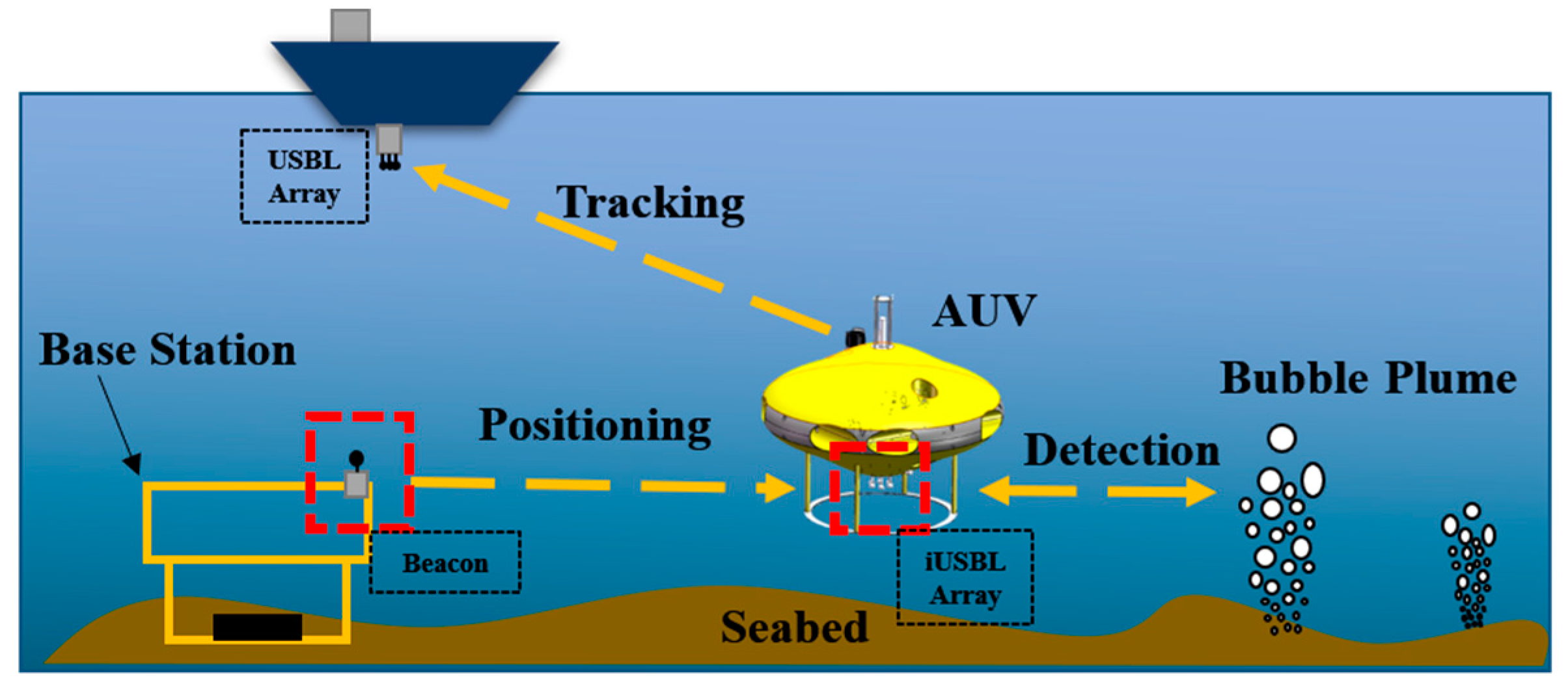
Ultra-short baseline (USBL) systems are commonly used for underwater acoustic positioning. They can be used to track subsea targets such as remote-operated vehicles (ROVs)/autonomous underwater vehicles (AUVs) or divers. Meanwhile, the USBL system can be employed for detecting and locating underwater targets, such as bubble plumes [1]. Alternatively, the USBL receiving array can be installed on the side of ROVs/AUVs in an inverted configuration called inverted USBL (iUSBL). This configuration allows the derived vehicle position to be used for AUV self-navigation. As an application example, Figure 1 shows an iUSBL-equipped disc-shaped AUV [2,3,4,5] that recently deployed in the South China Sea. In this application, the iUSBL provides position information that helps the AUV navigate to detect bubble plumes and find its way back to the base station. Additionally, another USBL installed below the vessel is used to track the AUV and locate the recovery position of the base station.

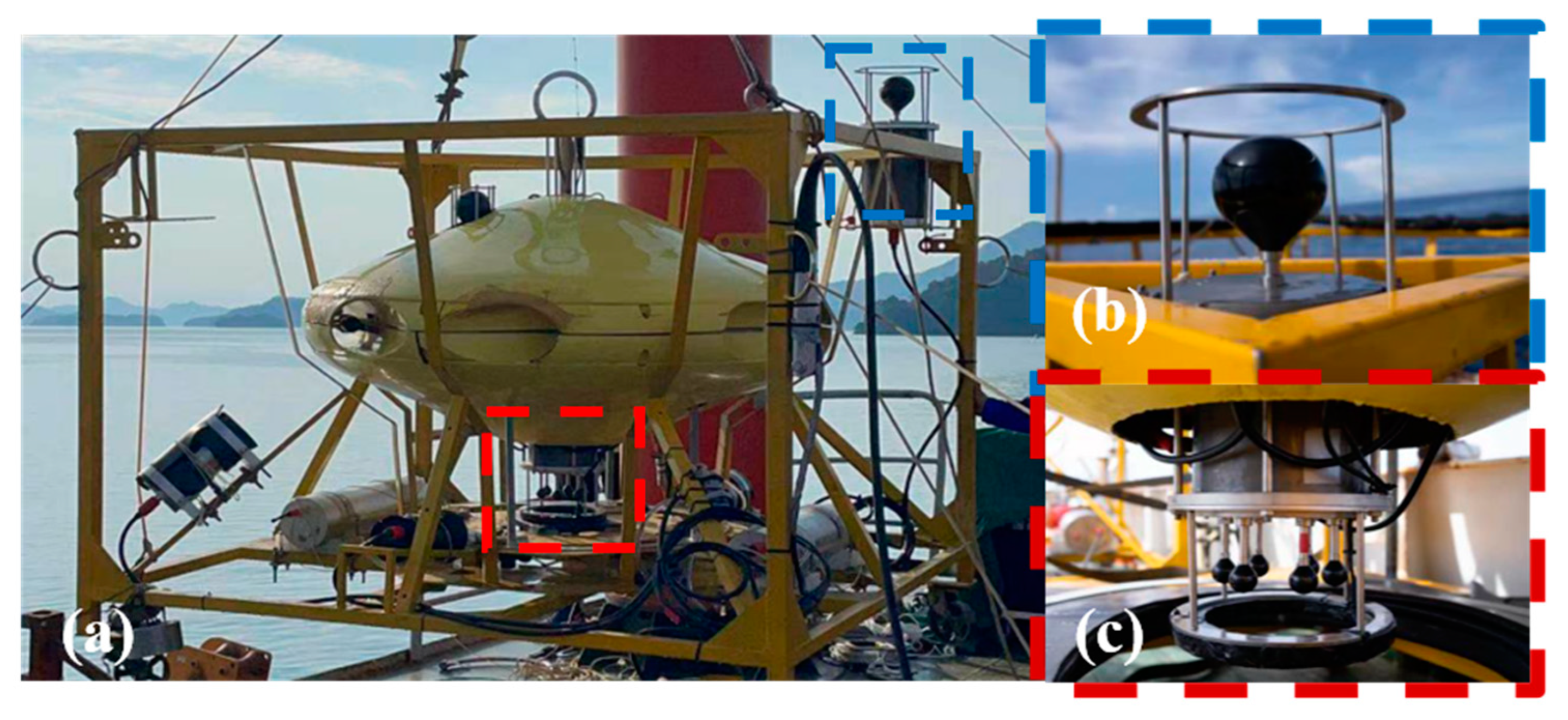
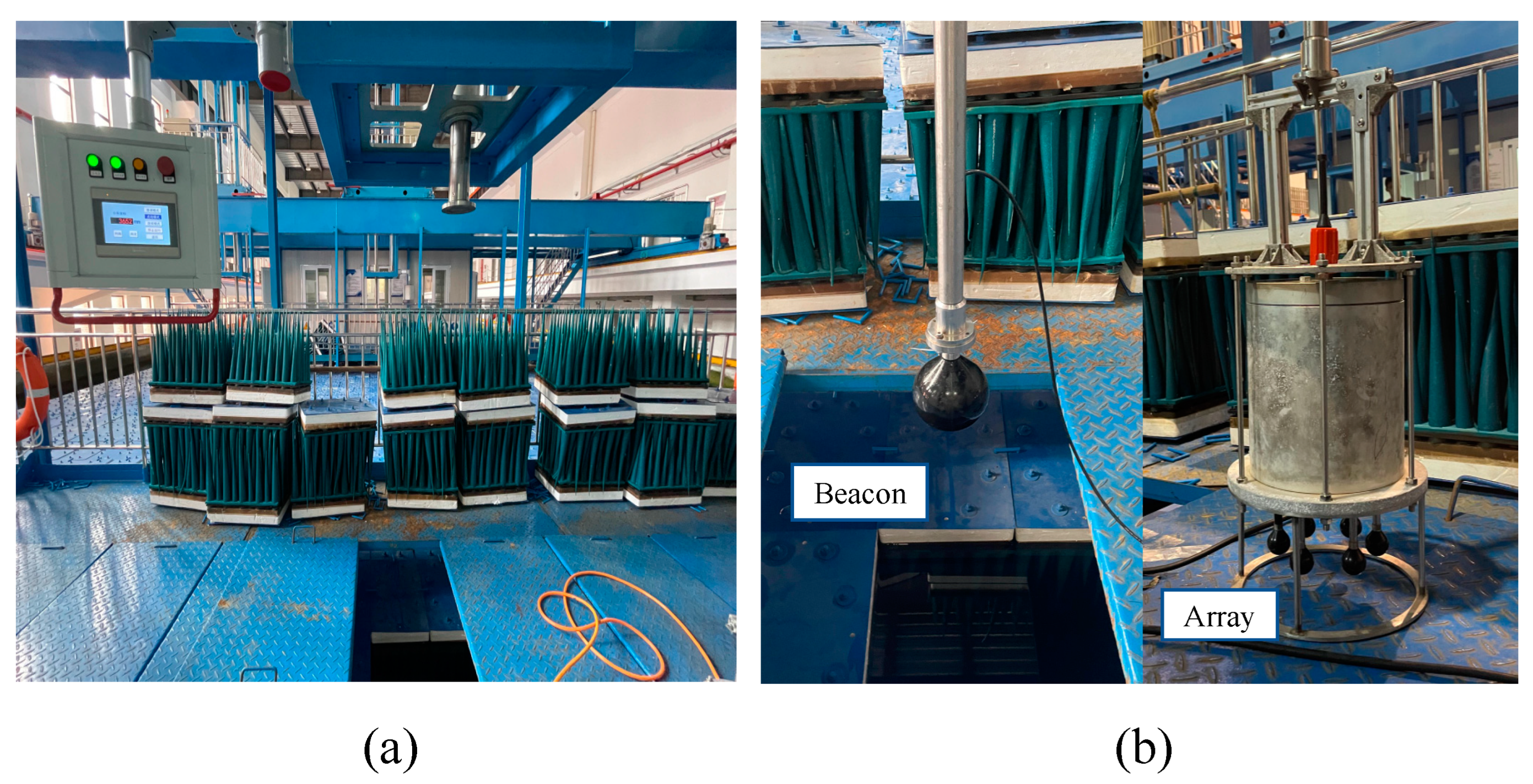
A broadband acoustic pulse is transmitted by the transmission beacon and detected by the USBL receiving array (pictures shown in Figure 2). The travel time between the beacon and the receiving array is then measured and converted into a range. The measured phase difference is applied to estimate the direction of arrival (DOA), also called “bearing”. Knowing the range and bearing, the relative position of the transmission beacon can be calculated. It should be noted that the position accuracy is mainly dependent on the bearing, especially for long-range applications.

Superdirective beamforming (SDB) [6,7,8,9] has gained much interest because it provides high angular resolution and a high directivity factor (DF). Theoretically, a small array, i.e., a USBL array, using SDB, can perform as well as a large array using conventional beamforming (CBF). Deconvolution beamforming (dCv) [6], as one of the SDB techniques, provides small beam widths, low sidelobe levels and a high DF while maintaining the robustness of CBF. Thus, the dCv-based superdirective USBL technique is expected to have higher bearing accuracy. However, this bearing accuracy still depends on many factors. For the environment, noise and multipath effects can directly degrade the signal quality [10,11]. For the array, imprecision in the hydrophone manufacturing process and array installation can reduce the bearing accuracy under ideal conditions [12].

The array error limits the upper accuracy limit of the system and must be calibrated before using the array. Array geometry errors (the actual position of the hydrophone deviating from the nominal position) have significant effects on positioning accuracy [13], and have been widely studied in microphone array calibration [14,15,16]. Initially, researchers used high-precision laser transit to locate each array element separately, but the high cost of optical equipment was prohibitive [17]. More recently, the goal of research has been to calculate the position of the array elements using only the captured acoustic signal, called acoustic geometry calibration or array self-calibration [12]. Pairwise distance (PD), time of arrival (TOA), and time difference of arrival (TDOA) measurements are often used for self-calibration [18]. For underwater array applications, conventional methods for distributed arrays, such as LBL arrays [19], do not apply to the calibration of USBL arrays. Reference [13] reduced the USBL elements spacing error to less than 1 mm, but the process was very complicated.

The equivalent receiving position of the hydrophone is called the acoustic center [20]. For better bearing performance, the acoustic response of each hydrophone is expected to be consistent, but unfortunately, this is not realistic [21]. Like microphones, whose acoustic centers are not always in the exact centers of the enclosing rubber ball [22], hydrophones can face the same problem. Reference [23] mentions that there is a directional offset in their USBL measurements, and they speculate that it is due to local acoustic interactions with the pontoons, but in fact, it is more likely due to array mismatch. Even if there is no installation error, the acoustic center of the hydrophone may not coincide with the geometric center. The mismatch depends not only on the electrical and mechanical features of the sensor, but also on its imperfect receiving pattern and the directivity of the received signal [24]. In addition, the acoustic center of the hydrophone may drift with rust and aging, and it is necessary to recalibrate after its replacement [25]. Reference [26] mentions that the additional phase shift introduced by USBL receivers could affect the phase difference measurement, but they only considered narrowband signals and ignored the different reception properties of hydrophones in each direction.

This paper introduces a fast calibration method for achieving high-precision calibration of superdirective USBL systems. In particular, the method addresses directional phase differences. In this paper, two error calibration models with different levels of complexity are proposed, and the effectiveness of the proposed method is verified by a series of tank experiments. After uniform phase delay calibration and non-uniform phase delay calibration, the system DOA estimation root mean squared error (RMSE) is reduced from 1.663° to 0.391° and 0.081°, respectively, and the maximum error is reduced from 3.5° to 0.7° and 0.2°. The results show that the calibration time cost can be significantly reduced from several hours to tens of minutes by choosing an appropriate rotation interval. Under this circumstance, the calibration accuracy can also be ensured.

This paper is organized as follows: Section 2 describes the beamforming method of the USBL system. Section 3 models the calibration model, and Section 4 discusses the calibration process for the two calibration models. The experimental results of the anechoic tank are analyzed in Section 5, which verifies the effectiveness of the calibration method. Section 6 discusses the possible causes of the non-uniform phase delay. The final section shows conclusions and future works.

2. Broadband Beamforming

CBF is a simple and robust beamforming method [27,28], but its beam pattern suffers from fat beams and high-level sidelobes, which makes it weak in multi-target applications and low signal-to-noise ratio (SNR) environments.

In principle, CBF assumes that plane waves from the far field hit hydrophones, which then delay-and-sum the signal for each channel. $H(\omega ,\theta )=e^{j\omega \tau }$ is equipped here to represent the delay matrix at a given look-angle $\theta$ and signal frequency $\omega$. To be specific, $\tau =d_i(\theta )/c$, where $c$ is sound velocity and $d_i(\theta )$ is the projection of the distance from the ith array elements to the origin on the look-angle $\theta$. So, the CBF output can be described as:

$$Y(\omega ,\theta )={\displaystyle \sum _{i=1}^N{H}_i(\omega ,\theta )}{X}_i(\omega )$$

(1)

where $X_i(\omega )$ is the Fourier-transformed signal received by hydrophone i. In the case of broadband beamforming, the CBF output power is usually the sum of the power over all frequencies. An l-length time series signal is subjected to a fast Fourier transform (FFT), corresponding to a frequency $f_k=k{f}_s/l$ at each sampling point, where $k$ is the frequency index. The power of broadband beamforming can be described as:

$${\left|B(\theta )\right|}^2=\frac{1}{M}{\displaystyle \sum _{k=1}^M{\left|Y({\omega }_k,\theta )\right|}^2}$$

(2)

where M is the length of the frequency index covering the broadband signal frequency.

Based on the determined beam pattern of the receiver array, the dCv deconvolves the CBF beam output to obtain a narrower beam width and a lower sidelobe-to-peak ratio [6]. However, the dCv algorithm is sensitive to the variation of the beam pattern because its approximation assumes that the beam pattern is only a function of $\theta -{\theta }_i$ and is independent of the target angles ${\theta }_i$, referred to as shift-invariant.

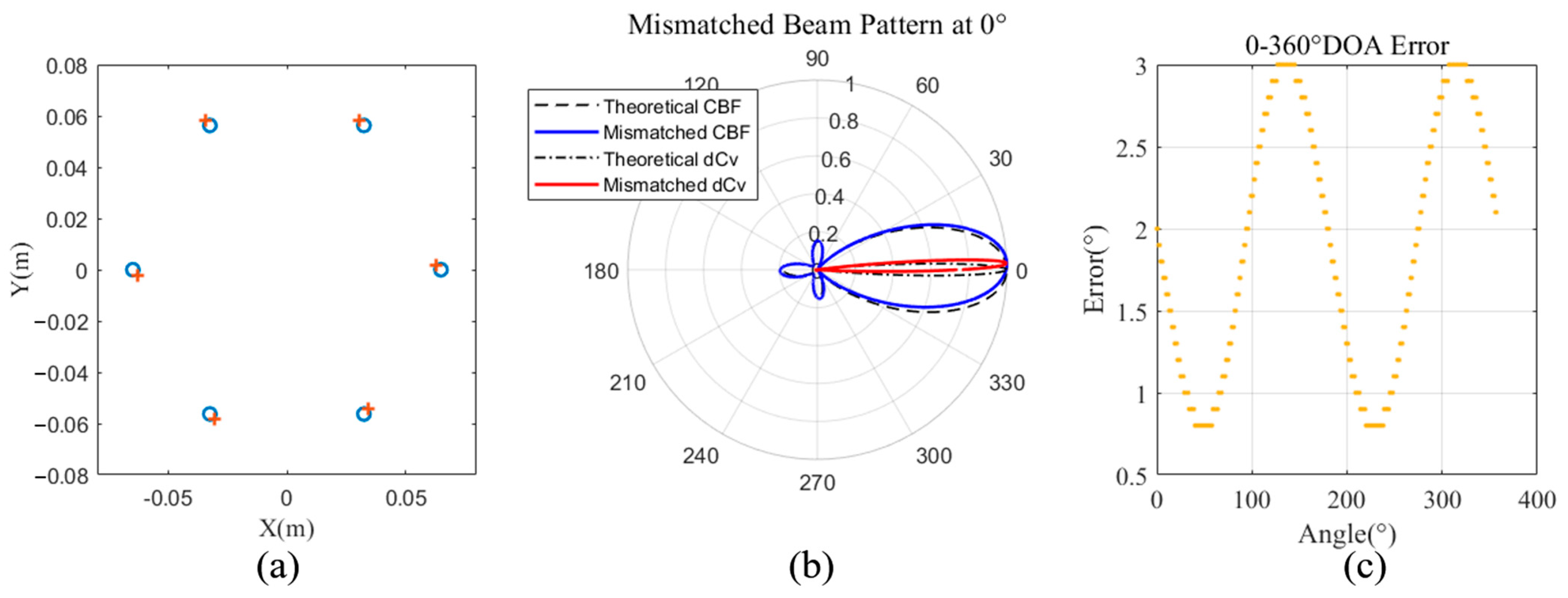
The dCv assumes that the CBF beam output has no significant distortion. However, even minor errors existing in array geometry may distort the CBF beam output, causing certain errors in estimated bearings. Taking our USBL array as an example, in Figure 3a, a random geometric error of 2 mm for each hydrophone is simulated. At this point, the mismatched array causes a distorted CBF beam pattern, and the dCv main lobe is still narrow but cannot reverse the effects of the mismatch, as shown in Figure 3b. Moreover, the DOA estimation error caused by the above geometric error is a function of the angle, as shown in Figure 3c. For our array, a geometric error of 3% of the array size would cause about a 2° bearing error, meaning a positioning error of 3.49% of the slant range.

3. Calibration Model

The geometry of the receiving hydrophone array is designed based on the deployment scenario in order to provide the best array beamforming performance. In theory, the incoming signal phase should be exactly the same for hydrophones, with the same diameter, located at the same nominal position. However, in the real world, there is inevitably a phase difference due to, for example, installation imperfections, inconsistencies inherent in the hydrophone manufacturing process, and/or varying delays in the receiving paths of the circuit board.

The circuit-induced phase difference may be the same for signals at all incoming directions, but hydrophone-induced phase difference may be a function of incoming signal direction. These factors are often mixed and cannot be discriminated easily. Hence, one considers these factors as a whole and calibrates these combined effects all at once. The effects of these mixing factors can be observed by measuring the signal arrival time difference for all hydrophone pairs. One uses a dual-hydrophone model to illustrate the calibration process for better understanding.

The phase differences among incoming signals mentioned earlier can be represented as time delays $t_d$ and equivalented to the distances shift $d$ at nominal sound velocity $c$.

$$d=t_d\cdot c$$

(3)

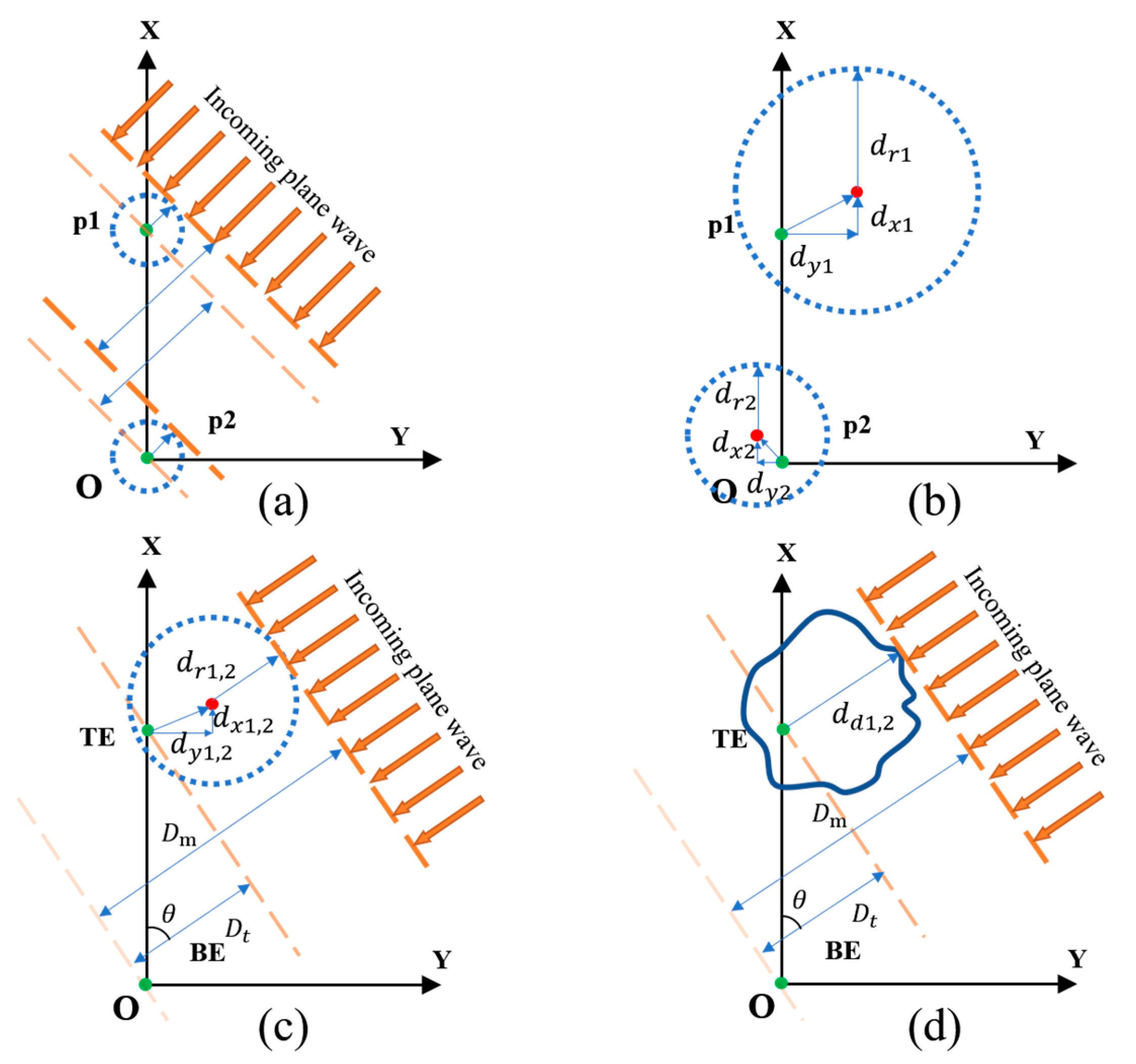
In general, Figure 4 depicts the calibration model and Figure 5 illustrates the calibration layout arrangement. To be specific, Figure 4a shows the ideal case with two ball-shaped hydrophones installed on the nominal position without installation error. Such hydrophones may be made with piezoelectric material with equal radii depicted with the blue dashed line. In this simplified two-hydrophone model, the green dot represents the geometric center of the hydrophone. The incoming plane wave from the far field hits the ceramic surface of the hydrophone and thus generates an electric signal from this moment. If all the array hydrophones have the same diameter, the delay from the ceramic surface to its geometric center is the same. The geometric center becomes the acoustic center in such an ideal case.

Often, this position can be physically shifted to the red-dot location (shown in Figure 4b) due to installation errors and/or hydrophone manufacturing inconsistencies. In addition, the circuit delay in each receiving path may be slightly different. This delay can be caused by, for example, the components used in the circuit board deviating from the nominal design value. Such delay deviation may be the same in all incoming signal directions but vary from channel to channel. For ball-shaped hydrophones, the equivalent diameter of the hydrophone varies from channel to channel, as shown in Figure 4b, depicted by the dashed line. In Figure 4b, $d_{ri}$ is modified from the nominal hydrophone radius, considering the additional contribution from each receiving path (receiving path depicted in Figure 5).

In order to perform DOA estimation in a superdirective USBL system, the phase differences between channels should be measured. The relative incoming signal phase delay in Figure 4b can be remodeled, as shown by Figure 4c. Here, the p2 hydrophone is considered to be a zero-phase point, called the Base Element (BE); thus, phase differences between the p1 hydrophone (known as the Target Element (TE)) and the BE can be measured. After converting the absolute offset shown in Figure 4b to the relative offset shown in Figure 4c, the p1 hydrophone can be modeled by an equivalent circle of radius $d_{r1,2}$ with a center shifted by $d_{x1,2}$ and $d_{y1,2}$.

For the incoming signal from angle $\theta$, the difference $E$ in the measured delay $D_m$ and nominal delay $D_t$ can be expressed by:

$$E(\theta )=D_m(\theta )-D_t(\theta )=d_{x1,2}\cos (\theta )+d_{y1,2}\sin (\theta )+d_{r1,2}$$

(4)

If one can estimate the relative hydrophone shift $d_{x1,2}$, $d_{y1,2}$, and equivalent radius $d_{r1,2}$, for all the TEs, the USBL array can be calibrated and achieve more accurate DOA estimation. In this calibration model, one needs only to store (N − 1) × 3 data in the system memory; thus, it is memory efficient for an embedded system.

However, the extra phase difference caused by hydrophone manufacturing differences does not guarantee directional consistency. Thus, the extra phase delay is not a circle of uniform radius, but a non-uniform one, as shown by the solid blue line in Figure 4d.

In the non-uniform model, the geometric center no longer has practical significance. The relative phase delay $d_{d1,2}$ between the relative equivalent receiver point and the nominal center is considered. The error can be simplified:

$$E(\theta )=D_m(\theta )-D_t(\theta )=d_{d1,2}(\theta )$$

(5)

$d_{d1,2}(\theta )$ can also be regarded as the acoustic characteristic distribution and the dual-hydrophone correction of the TE.

4. Calibration Method

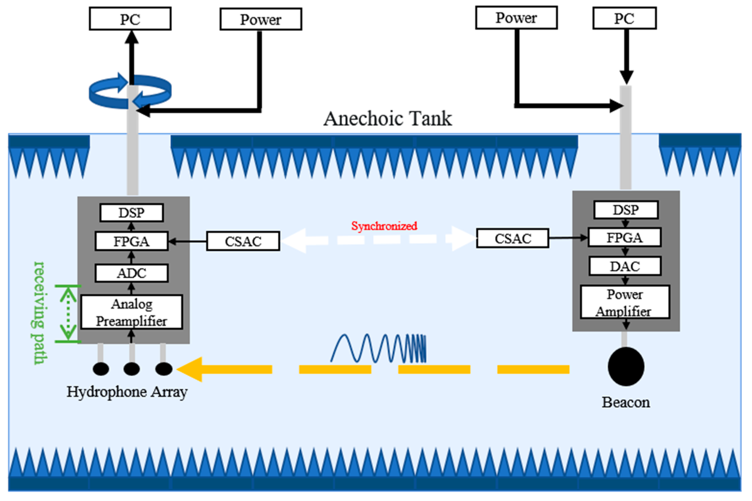
According to the calibration model established in the previous section, extra delay needs to be compensated to improve bearing accuracy. The calibration is performed in an anechoic tank, as shown in Figure 5, where a receiving array is attached to a rotatable shaft. This shaft can rotate by a small angle increment. The acoustic beacon is attached to another shaft at the same depth on the other side of the receiving array. The field-programmable gate arrays (FPGAs) at both ends are kept in time synchronization by chip-scale atomic clocks (CSACs), and the acquired signals are processed by digital signal processors (DSPs).

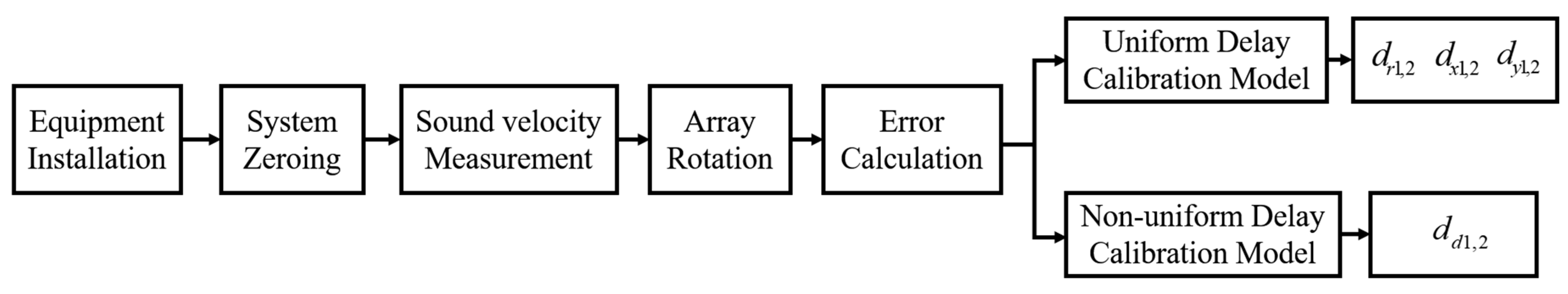
The calibration procedure is presented using a flow chart shown in Figure 6, including two models, named uniform delay calibration and non-uniform delay calibration, with different accuracy and complexity.

4.1. Error Calculation

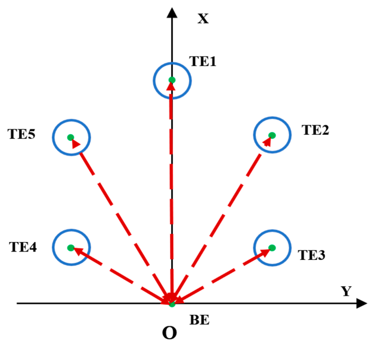
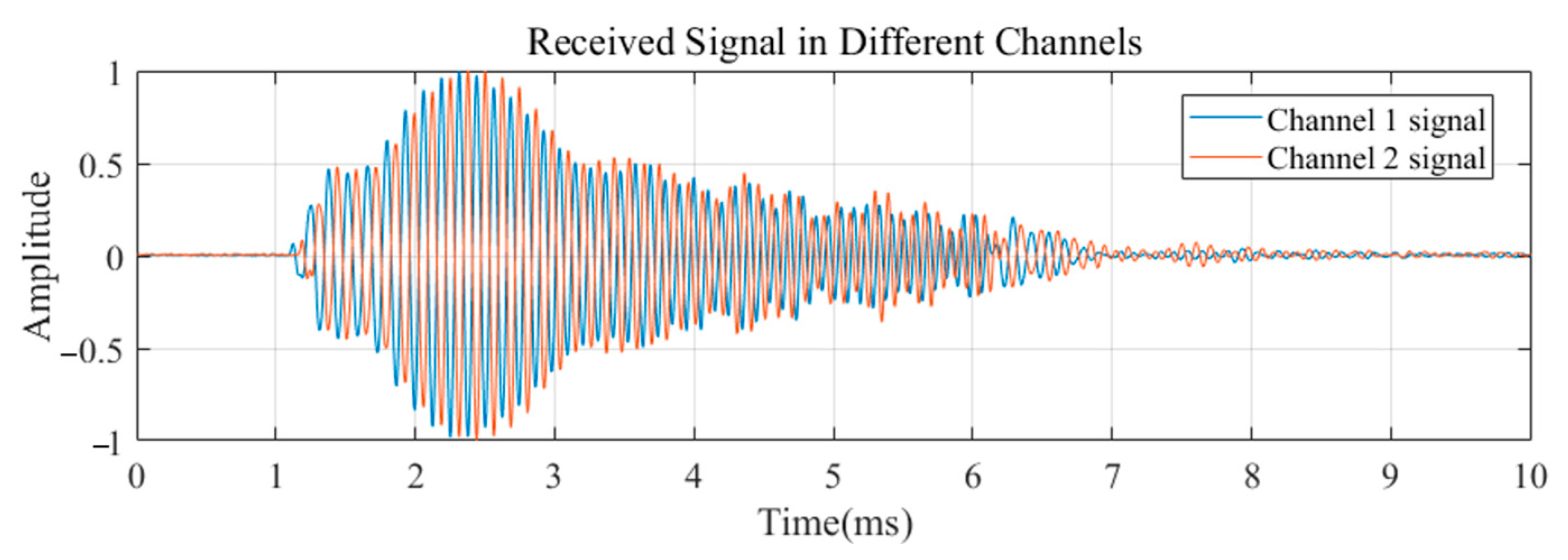
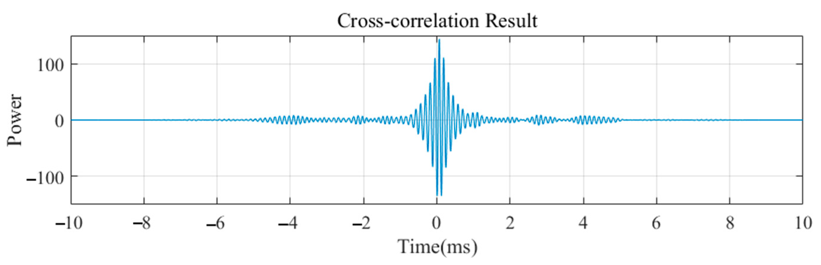
Any N-hydrophone USBL array can be decomposed into N − 1 hydrophone pairs, all with reference to the same BE. An example with a 6-hydrophone is shown in Figure 7. One may correct the delay in each pair separately. The received data are first oversampled for higher resolution, and time delays are obtained by cross-correlation with the transmitted signal. A 7–12 kHz linear frequency modulation (LFM) short pulse is chosen to get a sharp peak. The same signal is not only used for calibration purposes but also used for acoustic positioning for better consistency.

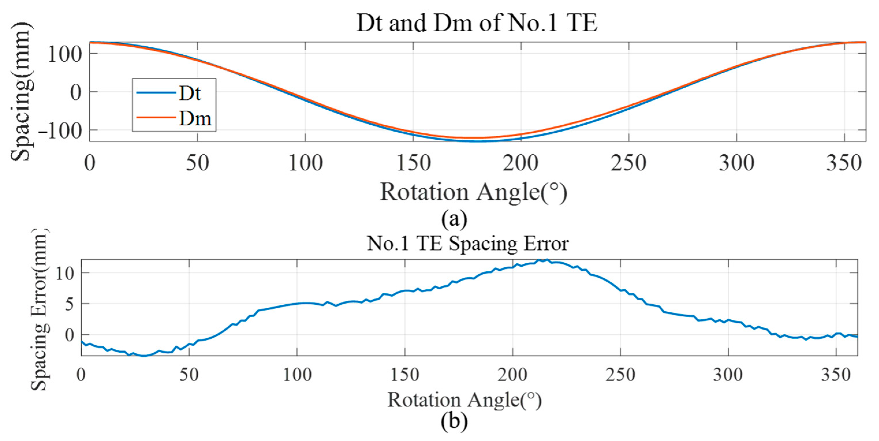
Figure 8 shows the received signals at the TE and BE hydrophones, respectively. The cross-correlation result of the TE channel is shown in Figure 9, and the peak time corresponds to the time delay caused by shaft rotation. When rotating the shaft, one will observe the $D_m$ curve through arrival time estimation while calculating the $D_t$ curve by the array geometry, as shown in Figure 10a. Both curves are not identical, and discrepancies exist, as shown in Figure 10b.

4.2. Uniform Delay Calibration

For geometrical errors in a given hydrophone, the signal delay at one angle can be compensated by an advance at the opposite angle. Hydrophone pairs, due to their symmetry in geometric position, can be used as mutual references and to avoid the introduction of additional reference hydrophones. According to (4), integrating $E$ from 0 to 2π eliminates the geometric offset. Then, the equivalent radius $d_{r1,2}$ can be calculated by taking the average:

$${\displaystyle \underset{0}{\overset{2\pi }{\int }}E}={\displaystyle \underset{0}{\overset{2\pi }{\int }}\left[d_{x1,2}\cos (\theta )+d_{y1,2}\sin (\theta )+d_{r1,2}\right]}=2\pi d_{r1,2}$$

(6)

$$〈{\displaystyle \underset{0}{\overset{2\pi }{\int }}E}〉=d_{r1,2}$$

(7)

where the geometric offset in 0–2π is integrated as 0, and the remaining differences, $E\prime =E-d_{r1,2}$, are all caused by the geometric offset.

$$E\prime (\theta )=d_{x1,2}\cos (\theta )+d_{y1,2}\sin (\theta )$$

(8)

$E\prime$ can be divided into the influence generated in the x-axis direction and the y-axis direction so that the offset in both directions at different angles can be calculated. Then, take the data received from two adjacent angles as a group, and rewrite (8) as a matrix equation:

$$\left[\begin{array}{c}{d}_{x1,2}\\ d_{y1,2}\end{array}\right]={\left[\begin{array}{cc}\cos ({\theta }_1)& \sin ({\theta }_1)\\ \cos ({\theta }_2)& \sin ({\theta }_2)\end{array}\right]}^{-1}\times \left[\begin{array}{c}E\prime ({\theta }_1)\\ E\prime ({\theta }_2)\end{array}\right]$$

(9)

An estimate of a pair of $d_{x1,2}$ and $d_{y1,2}$ can be determined by calculating sets of data by the least squares. Thus, all the parameters required for the uniform model $d_{x1,2}$, $d_{y1,2}$, and $d_{r1,2}$ are obtained. In this model, the computational complexity is O(N) and only (N − 1) × 3 data need to be stored.

In practice, it is impossible to know the relative delay of any angle. Instead, the approach involves rotating the array and uniformly sampling the calibration signal at small angular intervals. The interval angle should be as small as possible.

During CBF, a corrected array layout is used to replace the theoretical array. The theoretical position ($x_{t1}$,$y_{t1}$) of the TE position for the dual-hydrophone model is replaced by ($x_{t1}+d_{x1,2}$,$y_{t1}+d_{y1,2}$). For uniform delay, the equivalent radius $d_{r1,2}$ can be viewed as the phase difference of the signal received by the TE at each frequency ${\omega }_k$. Thus, the delay matrix H of (1) can be adapted, corresponding to an adapted phase of:

$$\delta {\phi }_k=e^{-j{d}_{r1,2}{\omega }_k/c}$$

(10)

where $\delta {\phi }_k$ is the phase adjustment of the signal at the kth frequency point, ${\omega }_k$ is the frequency at the kth frequency point.

4.3. Non-Uniform Delay Calibration

The uniform model considers only geometric offset and uniform delay, which can reduce the error of DOA estimation to some extent and requires less memory occupation for calibration data.

However, the uniform delay calibration ignores the effect of non-uniform delay. During the process of uniform delay calibration, the geometric offset causes hydrophone positions to move away from nominal positions. The array layout in beamforming is not consistent with the nominal layout, which will affect the beam pattern. For further high-precision calibration, more than the uniform model calibration is needed to improve the accuracy effectively.

Non-uniform delay calibration can avoid the insufficiency of uniform delay calibration. Referring to (1), CBF scans the look-angle from 0–2π and adjusts the phase delay according to the delay matrix of different angles. Since the correction quantity is also related to the incident angle of the signal, the $d_{d1,2}$ can be used as an additional quantity to add to the delay matrix $H$, and the corresponding adjusted phases are:

$$\delta {\phi }_k=e^{-j{d}_{d1,2}(\theta ){\omega }_k/c}$$

(11)

The non-uniform delay calibration completes the correction of the model and minimizes the effect of extra non-uniform delay. In this model, the computational complexity is O(N × n), where n is the number of look-angle numbers and (N − 1) × n data need to be stored. The higher the localization accuracy, the larger n is, which is not conducive to reducing the computational complexity to some extent.

5. Experiments and Results

To verify the calibration effectiveness of the methods, the USBL array is calibrated in an anechoic tank of 50 m × 15 m × 10 m, as shown in Figure 11. Specifically, connect the acoustic beacon and the six-element circular array with a radius of 0.065 m to two traveling cranes rigidly, and submerge them into the water at a depth of 1.5 m. Then, zero the traveling crane when the beacon and the array touch the water surface simultaneously. Additionally, coincide the USBL zero scale with the traveling crane zero scale. In this case, the rotation angle resolution of the traveling cranes is 0.1°, and the displacement resolution is 1 mm.

In the calibration layout arrangement shown in Figure 5, the shaft was rotated at 2° intervals and then received 7–12 kHz up-chirped 5 ms pulses. The sampling frequency $f_s$ was 200 kHz. To ensure a minimal time delay accuracy of 0.5 microseconds, approximately equivalent to 0.75 mm, the received signal was interpolated ten times. The beacon and the array were directly controlled by a PC via watertight cables so that data from the six channels could be processed in real time.

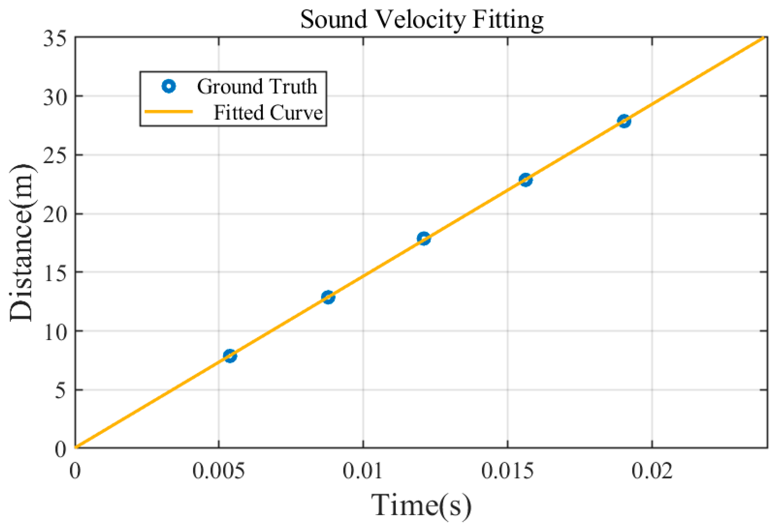
5.1. Equivalent Sound Velocity

First, the equivalent sound velocity (ESV) at a depth of 1.5 m was calculated, considering that the bending of sound rays at the same depth in a tank is negligible. After fixing the array, we moved the beacon away gradually by the traveling crane. Next, we sampled the matched filtering outputs of the calibration signal at intervals of 5 m. At each position, data were collected ten times and the average was calculated. Using least-squares fitting, the sound velocity of the tank was determined to be c = 1464.8 m/s, as shown in Figure 12.

5.2. Extra Phase Delay Measurement

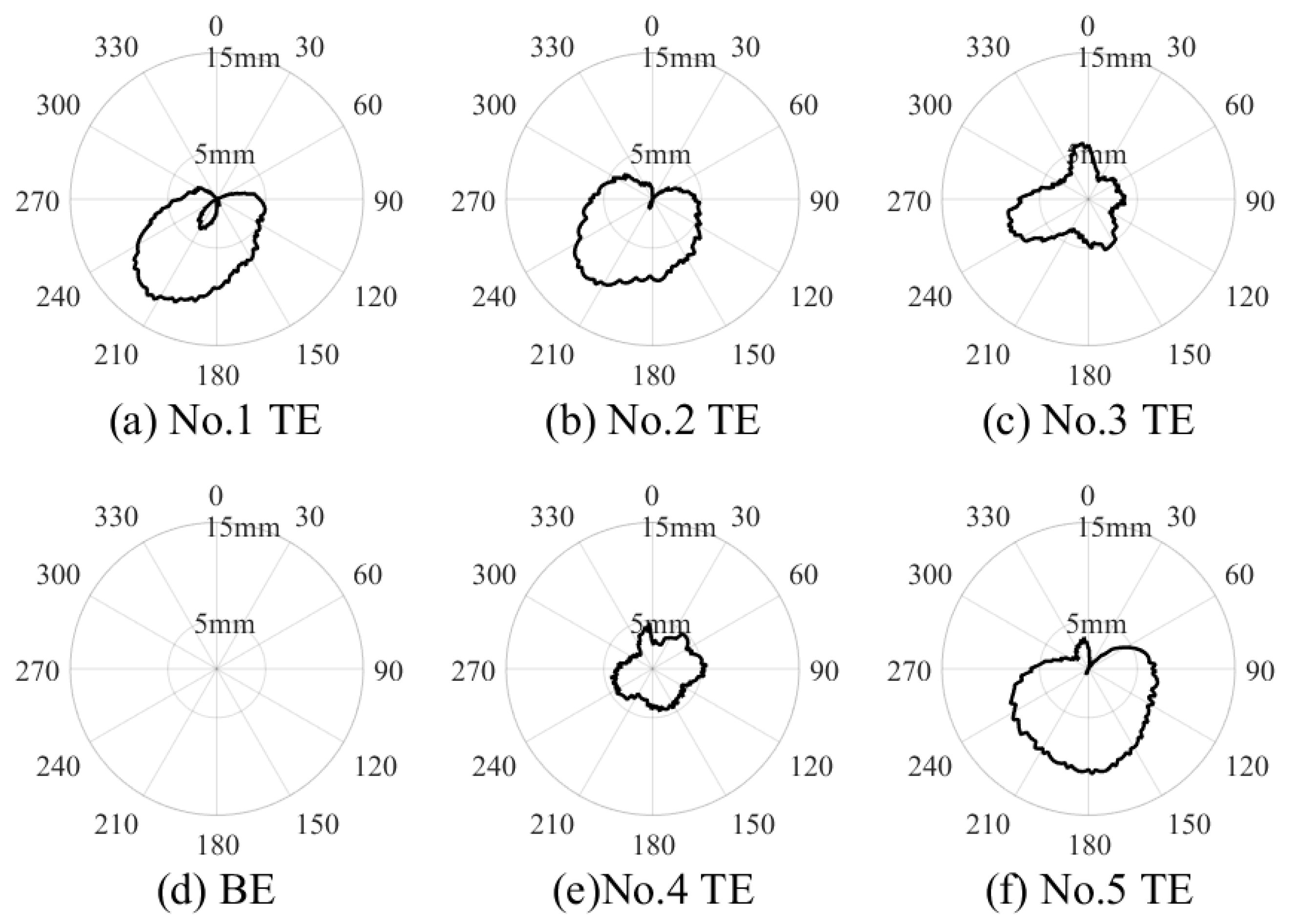
Initially, the 4th hydrophone in the six-element array was designated as the BE, while the other five elements served as TEs, as shown in Figure 7. Subsequently, we maintained the beacon at a distance of 27 m without it moving and continuously broadcast the calibration signal. At the same time, we rotated the array at 2° intervals. Following this, the calibration signals received by the array for each angle were recorded and the hydrophone pairs’ delay $D_m$ was measured. Furthermore, Figure 13 shows that the phase delay distribution is non-uniform, reflecting the difference in hydrophone performance to some extent. Notice that the phase delay in Figure 13d is 0 because we chose the 4th hydrophone as the BE, while the small circle inside the curve in Figure 13a represents a negative value near the 0° DOA, which is shown in polar coordinates in the opposite direction.

5.3. Array Calibration

According to the calibration model, the error of the BE is 0.

Table 1. Uniform delay calibration model parameters.

TE Number i	${\mathit{d}}_{\mathit{r}\mathit{i},4}$ (mm)	${\mathit{d}}_{\mathit{x}\mathit{i},4}$ (mm)	${\mathit{d}}_{\mathit{y}\mathit{i},4}$ (mm)
1	3.936	−5.894	−1.417
2	4.827	−4.170	−1.464
3	4.348	−0.611	−1.453
4	3.734	−0.324	0.886
5	5.722	−4.609	0.153

shows the calculated results of the offset errors and uniform delay of the TEs.

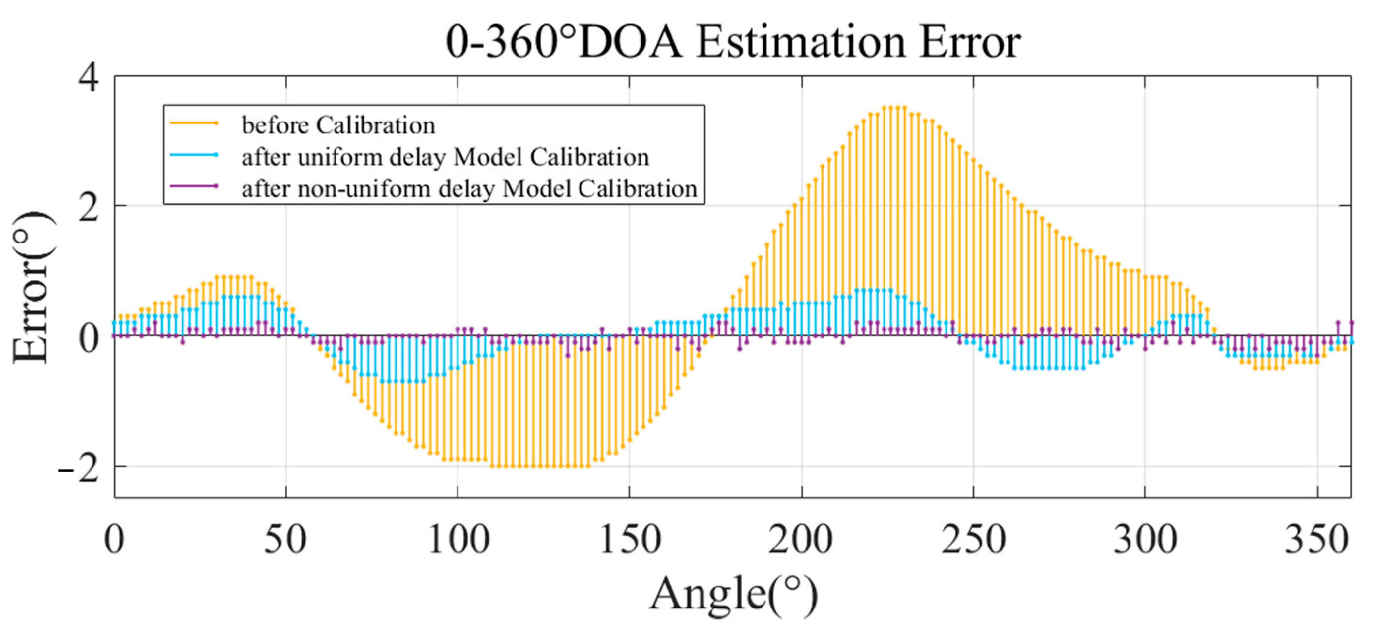
As shown in Figure 14, uniform delay model calibration effectively reduced the error to a sub-degree scale, but it is not perfect. Before the uniform delay model calibration, the RMSE of the system DOA measurement reached 1.663°. In comparison, it was significantly reduced to 0.3907°, and the max error was reduced from 3.5° to 0.7°. However, there were still some apparent errors in some angles that the uniform delay model could not correct.

Due to the high time cost, it was almost impossible to record the difference E at 0.1° array rotation intervals, which meant that we could not match the index angle to the correction volume. Therefore, we used three splines to interpolate the 2° interval data of the delay distribution (shown in Figure 13) to the 0.1° interval.

Finally, we adjusted the signal phase according to the corresponding correction volume amount to complete the calibration. The non-uniform delay model calibration error is shown in the purple line in Figure 14, and the RMSE is further reduced to 0.081°. It shows that most of the absolute errors can be controlled within 0.2°, which significantly improves the DOA measurement accuracy of the system.

5.4. Effect on Beam Pattern

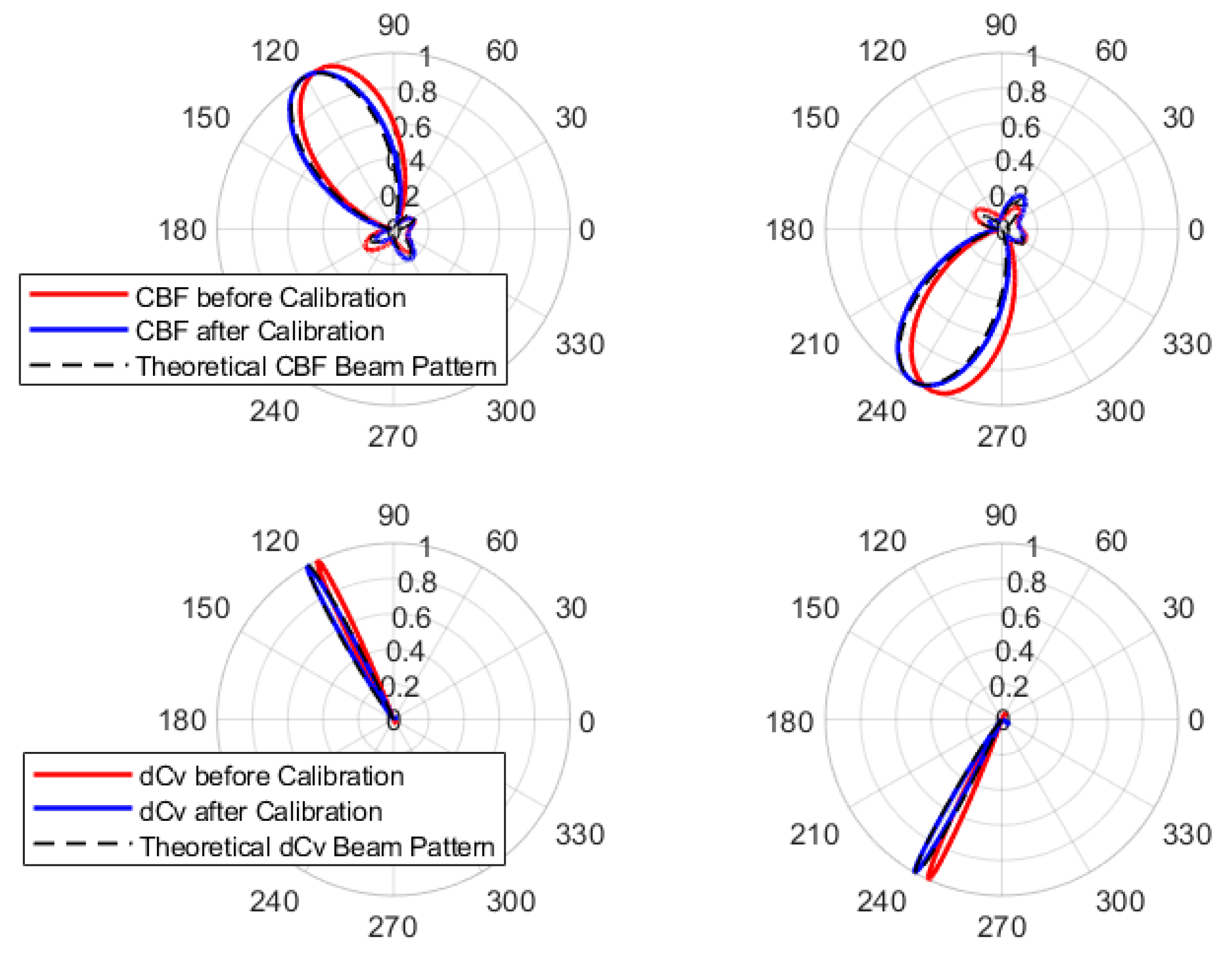
For CBF, the extra phase delay causes signal mismatch, so the maximum value of the beam pattern deviates from the theoretical angle, and the CBF beam pattern is distorted. As shown by the red line in Figure 15, the CBF beam pattern deviated from the theoretical beam pattern shown by the black dashed line. In this way, the DOA estimation of the CBF is incorrect. Moreover, the dCv beam pattern is also significantly affected, as shown in the bottom two panels of Figure 15. This is highly detrimental to the ability to exploit the high-resolution performance of the dCv.

After the correction, it is clear that the beam pattern of the CBF is improved, and the blue line in the figure more basically coincides with the dashed line of the theoretical beam pattern. As a result, the dCv beam pattern improves and returns to near the theoretical position. This result demonstrates that the correction for the non-uniform phase delay can significantly correct the distorted beam pattern and improve the accuracy of DOA estimation.

5.5. Time Spent on Calibration

The most time-consuming step in the process is to rotate the array. In order to reduce the time spent on calibration, we investigated the effect of rotation angle interval on time spent on calibration.

The angle interval of the array rotation is inversely proportional to the number of measurement points. The more measurement points there are in the calibration process, the more time it takes. Usually, the goal is to encompass a wide range of angles, but this takes a lot of time. The minimum angle interval we chose for our experiment was 2°, so we needed to measure at least 180 angles, which took us almost an hour.

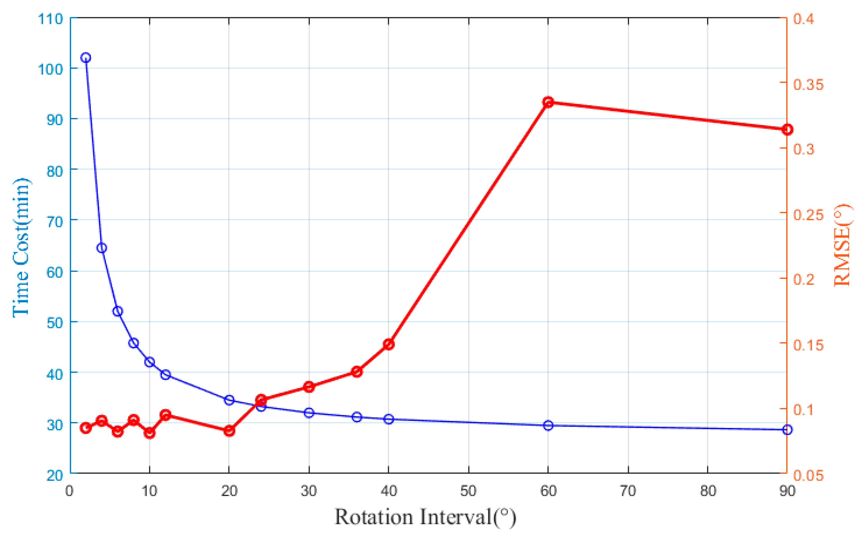
In the experiments, calibration was attempted using various rotation intervals, and the subsequent improvements in corrected DOA estimation errors are compared. As shown in Figure 16, we used the data at 2° intervals as a base and selected data at large intervals. To be specific, we assumed that the rotation interval was 4°, 6°, 8°, and higher to 90°, and performed a calibration process to compare the standard error of 0–360° after calibration.

An observed trend was that as the rotation interval increased, the error also showed an increase. The bearing RMSE was kept within 0.1° when the interval was less than 20°, which meant that the calibration accuracy met expectations.

The time cost in Figure 16 includes the necessary device commissioning time of about half an hour and rotational measurement time, scaled according to the time recorded in the experiment. As a result, by adopting this approach, calibration can be performed at 20° intervals, requiring measurement at only 18 points—ten times fewer than the initial measurement points. In this case, the calibration time can be reduced from the original 102 min to 34 min. And, we simulated the calibration with the method of literature [13], which takes about 270 min, and the comparison shows the significant improvement in the time efficiency of the new method.

From the comparison results, the calibration accuracy is not significantly reduced by appropriately relaxing the measurement interval. However, the calibration time overhead can be significantly reduced because the non-uniform phase delay varies slowly with the angle. If the phase delay changes rapidly, a reduction in the measurement interval should be considered.

6. Discussion

It has been previously reported that deconvolution is very effective in suppressing the sidelobes (despite hydrophone position errors), but it cannot correct the bearing bias caused by such errors [6]. Therefore, for dCv-based USBL systems, the signal mismatch caused by phase distortion has to be compensated carefully. Figure 13 also shows that the phase delays (relative to BE) are non-uniform and can be represented as a function of incoming signal direction. The possible reasons for such bearing-dependent array errors include:

• Installation-induced errors:

The installation error only affects the geometric position of the array elements and does not produce a non-uniform component.

Our hydrophones are rigidly attached to a precision-machined aluminum pressure housing, which has almost no offset. However, it cannot be ignored that a slight bending of the rod can also produce geometric offsets, which are difficult to observe.

• Receiving path inconsistency:

There are many inductive components in the signal sampling circuit, and tiny differences between the preamplifier circuits of each channel can produce phase differences. Most of the uniform phase delay errors are generated by the circuit phase differences. Therefore, before connecting the hydrophone, the phase difference generated by the circuit needs to be eliminated. Before the experiment, we also calibrated the preamp circuit to ensure that the phase between the channels was as uniform as possible.

• Inconsistency in the hydrophone manufacturing process:

In comparison, a more reasonable explanation is the response error inherent in the hydrophone manufacturing process. If the sensing elements of a hydrophone are physically unevenly distributed in the housing, there must be differences in the response to sound in all directions. There may also be phase inconsistencies in the internal components of the hydrophone.

7. Conclusions

This paper proposed a fast calibration method for a superdirective USBL system. The method is to fix the acoustic beacon and the array in an anechoic tank and rotate the array in small angular increments. To verify the effectiveness of this method, we conducted an anechoic tank experiment on the six-element circular array of a USBL system. The results indicate that the uniform delay model calibration can reduce the DOA estimation error to the sub-degree level, and the non-uniform delay model calibration can effectively reduce the maximum DOA error of the system from 3.5° to 0.2°, and the corrected RMSE can reach 0.081°. Meanwhile, the calibration of the dCv can be performed at the beam pattern level, which in turn improves the bearing accuracy. At the same time, the calibration time can be reduced from several hours to tens of minutes while still meeting the application requirements.

In the future, we plan to conduct fast calibration in the field, which is beneficial to get rid of the constraint of the anechoic tank in the laboratory and the need for the rapid transplantation of USBL systems. In this circumstance, the lack of a high-precision traveling crane is unsuitable for determining calibration accuracy, which could be another problem. Furthermore, it would be of great interest to fit ESV by differential GPS in the field or to measure ESV directly using the calibrated array.