A Study of Combined Graphical Acoustic Computing and the Depth Peeling Technique on Acoustic Backscattering of Multiple-Layered Structures

Abstract

An efficient graphical acoustic computing (GRACO) method is introduced. Referring to the rendering of semi-transparent objects, the depth peeling (DP) technique is compounded with the GRACO method, forming a combined GRACO and DP method (GRACO–DP) to consider the backscattering of multiple-layered structures in which the contributions of inner structures are included. After that, some examples of GRACO and GRACO–DP are tested to evaluate the accuracy and efficiency of such methods. Through the examples of impedance sphere and benchmark models, GRACO can acquire results with higher efficiency and good consistency compared to the traditional KA method. Also, the TS of a pair of circular plates is determined by GRACO, GRACO–DP, and the finite element method (FEM). The results show that GRACO–DP can fit better with the FEM results. Moreover, the TS of a ribbed double shell is predicted by both GRACO and GRACO–DP; the features of a Bragg wave scattered by the periodically arranged inner ribs can be spotted from the result of GRACO–DP.

1. Introduction

Underwater vehicles are extensively utilized devices in ocean resource exploration and marine defense technology. Due to sonar detection and acoustic stealth demand, acoustic backscattering issues of both underwater vehicles and detecting targets are always drawing concerns from researchers in this field. In this work, the ribbed double cylindrical shell, which is a commonly used structure in underwater vehicles, is chosen as the target to discuss the acoustic backscattering of structures with multiple-layered shells, the outer surfaces of which incident acoustic waves can penetrate through and the existence of inner structures can make contributions to total backscattering.

The research on acoustic backscattering dates back to the works of Rayleigh [1]. He initiatively gave a mathematical expression of the scattering of sound. Due to the limitation of the complexity of the expressions, he only considered some simple cases in which the size of the scatterer was relatively small compared to the incident wavelength. Based on Rayleigh’s work, considering the limitation on scatterer size, Morse [2,3] applied partial wave series (PWS) to separate the complicatedly dependent variables in the Helmholtz equation and the acoustic scattering solution of some simple scatterers like a rigid sphere and an infinite cylinder in a liquid medium was acquired. Following Morse’s works, Faran [4] and Junger [5] extended the PWS into the backscattering prediction of elastic scatterers like isotropic cylinders/sphere solids and shells. They found that for scatterers whose density is greater than the liquid external medium, if the incident wave frequency is higher than the first-order free-vibration mode of the scatterer, the scattering pattern of the elastic scatterer no longer fit with the rigid counterpart and the scattering pattern of the elastic scatterer changed drastically when a small change in frequency occurred in the vicinity of the scatterer’s free-vibrating modes.

Due to the limitation of analytical methods imposed on the scatterer’s geometry, some numerical and semi-numerical methods were developed. Stanton [6,7,8] proposed the deformed cylinder method (DCM). This method can cope with the scattering of deformed cylinders of finite length and, thus, most ocean objects such as marine organisms, sand ripples, and ice keels can be considered by this method as they can be approximated as elongated objects. Another frequently applied semi-numerical method is the Transition matrix (T-matrix) method proposed by Waterman [9,10] to cope with the backscattering of rigid and elastic scatterers. Recently, Gong proposed applications of this method to the backscattering issues of spheroid and capsule-shaped structures [11,12]. Although great efforts have been made by these semi-numerical methods, the shape of the considered scatterers is still limited in variety. With the rapid development of the finite element (FEM) and boundary element methods (BEM), these two methods were introduced to the acoustic field and vastly applied in studying backscattering problems of all kinds of objects [13,14,15,16,17,18]. Benefiting from the fruitful theoretical foundations of these methods, the backscattering of complex scattering in complex conditions can be determined easily. Recently, some extended methods like the smooth finite element method (SFEM) and meshfree method have been applied [19,20,21,22,23,24,25,26,27]. Although the flexibility of these methods can never be worried about, there is a common disadvantage of these rigorous numerical methods in that the efficiency of these methods plunges sharply with an increase in frequency due to the fact that refined meshed is necessary for high-frequency models.

Considering the efficiency of high-frequency and large-scale models, an asymptotic method called the Kirchhoff approximation (KA), also known as physical acoustics (PA), is introduced. The KA regards the backscattering of the scatterer as the Helmholtz integration of the illuminated regions. Urick [28] referenced Kerr’s [29] work on the radar cross section and gave the backscattering target the strength of some rigid simple structures using the KA. Later, Gordon [30] worked out the explicit expression of the Helmholtz integration of a flat polygonal element, and his contribution made it possible to approximate the total backscattering of an arbitrary surface as the sum of a series of planar elements. Fan [31,32] solved the discretized KA models with Gordon’s integration, and the planar element method (PEM) was formed to efficiently cope with the backscattering of large-scale and high-frequency models. Since the expression of Gordon’s integrations is independent between elements, the integration procedure of the discretized KA can be easily processed through a parallel program. In the electromagnetic field, the computer 3D graphical rendering technique is introduced to parallelly consider electromagnetic scattering [33,34]. Likewise, this thought is introduced to the acoustic field to form the graphical acoustic computing (GRACO) method [35,36]. Aided by the efficient and reliable graphical rendering technique, the time cost of KA is shortened to a striking degree.

In the current work, GRACO is applied to study the backscattering issues of multiple-layered structures. The ribbed double shell is taken as an example. In many previous works of research on KA-based backscattering issues, the scatterer is regarded as a rigid or impedance surface. The acoustics cannot penetrate through the outer surface of the scatterer. Thus, the contribution of the inner structure is usually abruptly overlooked. In this paper, the depth peeling (DP) technique [37], which is usually used to cope with the rendering of semi-transparent objects, is combined with the traditional GRACO method to deal with the backscattering of multiple-layered structures.

The remainder of this paper is organized as follows: In Section 2, a brief introduction of the Kirchhoff approximation is given; additionally, the discretized scheme of the traditional KA as well as the GRACO method are introduced; moreover, the hidden surface elimination operations of the traditional routine and Z-buffer are compared; at last, the implementation of DP into GRACO is briefed. In Section 3, the target strength of some examples such as a sphere, a benchmark, a pair of circular plates, and a ribbed double shell is considered with different methods, and the results of different methods are compared to narrate the advantages of GRACO–DP. In Section 4, the conclusions are given.

2. Theories and Methods

2.1. The Integral Equation and the Kirchhoff Approximation

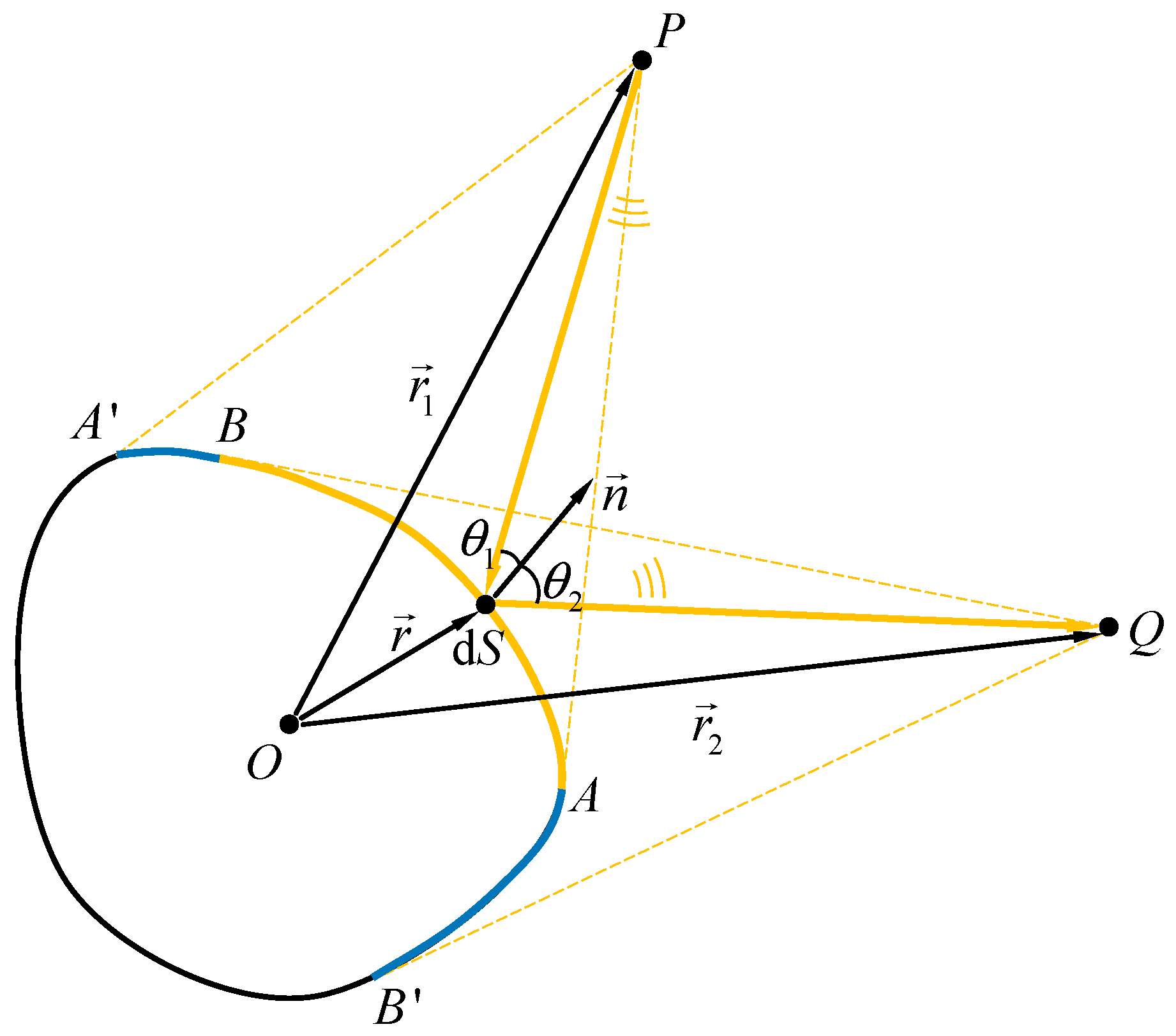
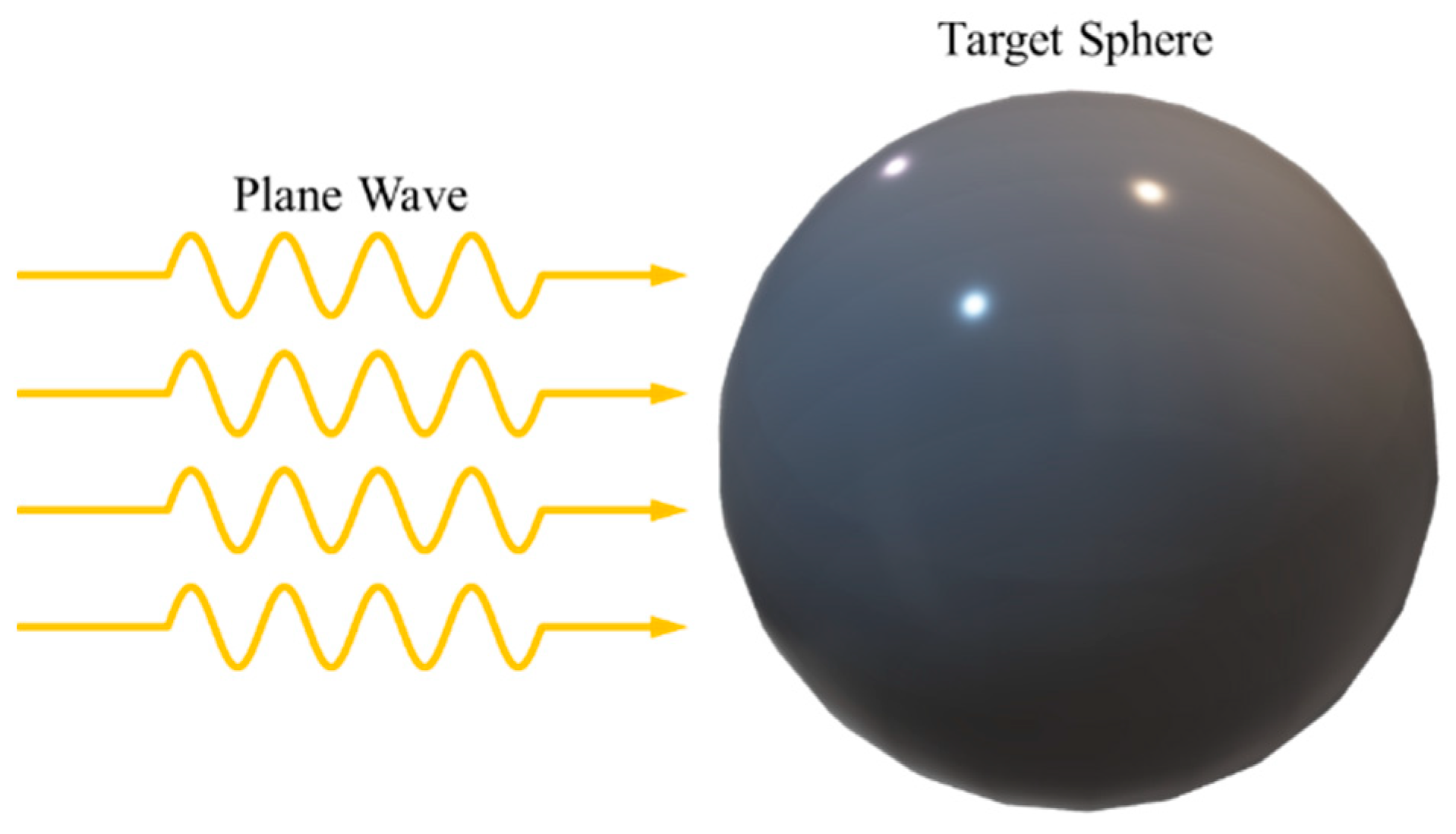
As shown in Figure 1, an object with surface S is insonified by a far-field point source P. The incident velocity potential over the target surface is

$${\varphi }_i\left(\overrightarrow{r}\right)=\frac{e^{ik\left|{\overrightarrow{r}}_1-\overrightarrow{r}\right|}}{\left|{\overrightarrow{r}}_1-\overrightarrow{r}\right|},$$

(1)

where k is the acoustic wave number in water. According to the Kirchhoff integral equation of acoustic scattering [3], the scattering potential at observation point Q is

$${\varphi }_s\left({\overrightarrow{r}}_2\right)=\frac{1}{4\mathsf{\pi }}{\displaystyle \underset{S}{∯}\left[{\varphi }_s\left(\overrightarrow{r}\right)\frac{\partial }{\partial n}\left(\frac{e^{ik\left|{\overrightarrow{r}}_2-\overrightarrow{r}\right|}}{\left|{\overrightarrow{r}}_2-\overrightarrow{r}\right|}\right)-\frac{\partial {\varphi }_s\left(\overrightarrow{r}\right)}{\partial n}\left(\frac{e^{ik\left|{\overrightarrow{r}}_2-\overrightarrow{r}\right|}}{\left|{\overrightarrow{r}}_2-\overrightarrow{r}\right|}\right)\right]\mathrm{d}S}.$$

(2)

There is usually no analytical solution for an object with a complex shape according to Equation (2). Thus, the Kirchhoff approximation (KA) is a frequently used method to cope with complex-shaped models. In the KA, there are two hypotheses included to simplify the acoustic scattering model: (1) only the scattering contribution of the illuminated region is considered; (2) the tangent plane approximation. Only considering the illuminated region means that the shadowed region $\stackrel{⌢}{A{}^{\prime }B{}^{\prime }}$ and the penumbra regions $\stackrel{⌢}{AB{}^{\prime }}$ and $\stackrel{⌢}{A{}^{\prime }B}$ are excluded from the integral area, and the total scattering integration can be approximated by integration over the illuminated region:

$${\varphi }_s\left({\overrightarrow{r}}_2\right)\approx \frac{1}{4\mathsf{\pi }}{\displaystyle \underset{S_{\stackrel{⌢}{AB}}}{\iint }\left[{\varphi }_s\left(\overrightarrow{r}\right)\frac{\partial }{\partial n}\left(\frac{e^{ik\left|{\overrightarrow{r}}_2-\overrightarrow{r}\right|}}{\left|{\overrightarrow{r}}_2-\overrightarrow{r}\right|}\right)-\frac{\partial {\varphi }_s\left(\overrightarrow{r}\right)}{\partial n}\left(\frac{e^{ik\left|{\overrightarrow{r}}_2-\overrightarrow{r}\right|}}{\left|{\overrightarrow{r}}_2-\overrightarrow{r}\right|}\right)\right]\mathrm{d}S}.$$

(3)

The tangent plane approximation suggests that the scattering character of the points on the scatterer surface is approximated to a cluster of planar elements with the properties of infinite tangent planes. Therefore, the scattering velocity potential on the target surface can be approximated by the reflecting model of an infinite plane insonified by the plane wave

$${\varphi }_s\left(\overrightarrow{r}\right)=V\left({\theta }_1\right){\varphi }_i\left(\overrightarrow{r}\right),$$

(4)

where $V\left({\theta }_1\right)$ is the reflection coefficient at the scattering point and ${\theta }_1$ is the angle between the vector of the incident wave and the normal of the scattering point. Furthermore, the ratio of total acoustic pressure to total normal vibration velocity at the surface is equal to the acoustic impedance of an infinite plane:

$$\frac{i\omega \rho \left[{\varphi }_i\left(\overrightarrow{r}\right)+{\varphi }_s\left(\overrightarrow{r}\right)\right]}{\partial \left[{\varphi }_i\left(\overrightarrow{r}\right)+{\varphi }_s\left(\overrightarrow{r}\right)\right]/\partial n}=-Z_n,$$

(5)

where ω and ρ are angular frequency and water density, respectively, and Z_n is the acoustic impedance of the target surface. The relation between the acoustic impedance and the reflection coefficient can be expressed as

$$\frac{\rho c/\cos {\theta }_1}{Z_n}=\frac{1-V\left({\theta }_1\right)}{1+V\left({\theta }_1\right)},$$

(6)

where c is the water acoustic velocity. Substituting Equations (4)–(6) and Green’s function into Equation (3), the acoustical velocity potential of receiving point P can be expressed as

$${\varphi }_s\left({\overrightarrow{r}}_2\right)\approx -\frac{ik}{4\mathsf{\pi }}{\displaystyle \underset{S_{\stackrel{⌢}{AB}}}{\iint }\frac{e^{ik\left(r_1+r_2\right)}}{r_1{r}_2}{e}^{-ik\left(\overrightarrow{r}\cdot \frac{{\overrightarrow{r}}_1}{r_1}+\overrightarrow{r}\cdot \frac{{\overrightarrow{r}}_2}{r_2}\right)}V\left({\theta }_1\right)\left(\cos {\theta }_1+\cos {\theta }_2\right)\mathrm{d}S}.$$

(7)

For the backscattering problem, the source point P and the observation point Q are at an identical position, and the variables related to P and Q can be combined together. That means, ${\overrightarrow{r}}_1={\overrightarrow{r}}_2={\overrightarrow{r}}_s$ and ${\theta }_1={\theta }_2=\theta$. Therefore, the scattering velocity potential at the observation point can be expressed as

$${\varphi }_s\left({\overrightarrow{r}}_s\right)=-\frac{ik}{2\mathsf{\pi }{r}_s^2}I,$$

(8)

where

$$I=e^{2ik{r}_s}{\displaystyle \underset{S_{\stackrel{⌢}{AB}}}{\iint }{e}^{-2ik\overrightarrow{r}\cdot \frac{{\overrightarrow{r}}_s}{r_s}}V\left(\theta \right)\cos \theta \mathrm{d}S}.$$

(9)

The backscattering velocity potential can be obtained with the integration of Equation (9). For a target surface of complex shape, the integration of Equation (9) cannot be obtained directly. Some discretization techniques can be applied to simplify the complex surface into a series of simple planar elements and the scattering potential integral can be acquired by summing up the integrations over each element. In an underwater sonar system, the target strength (TS) is a much more commonly used parameter to describe the stealth of the underwater target. It is defined as the log value of the ratio between the equivalent backscattering acoustic intensity at a position one unit of distance from the acoustic center and the incident acoustic intensity at the acoustic center:

$$\mathrm{TS}=20\log {\displaystyle \underset{r\to \infty }{\lim }}\left|\frac{ik}{2\mathsf{\pi }}I\right|.$$

(10)

where $I_s$ is the acoustic intensity of the scattering field, $I_i$ is the incident acoustic intensity, ${\overrightarrow{r}}_O$ is zero vector, ${\overrightarrow{r}}_P$ is the vector from the origin O to the source (observation) point P, $r_0$ = 1 m is the unit length and is omitted here due to the SI used in the current study. For simple shapes, the integration of I can be easily solved. However, when coping with complex surfaces, it is impossible to acquire the integration over these surfaces, and some discretization technique is needed to simplify this problem. What should be mentioned is that the $\left|e^{2ik{r}_s}\right|$ is not deleted in the integration of I. This is because in the following discretization procedures, the reference point of different elements varies, and the $e^{2ik{r}_s}$ term generates a phase difference between different elements.

2.2. The Discretization Schemes for Kirchhoff Approximation

2.2.1. The Planar Element Method

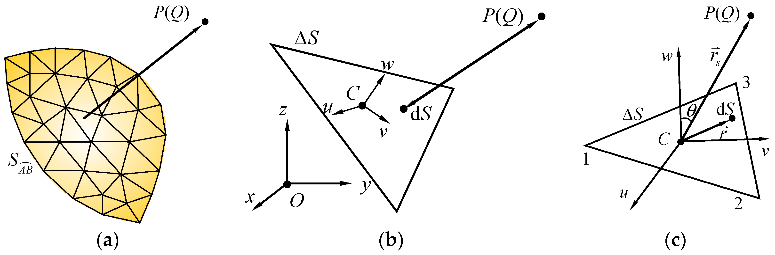
As shown in Figure 2a, an arbitrarily shaped surface can be discretized by a series of elements, and in the following discussions, triangular elements are taken as an example to introduce the planar element method. Thus, the integral part I can be equalized as the summation of integrals on every individual element:

$$I={\displaystyle \sum \mathsf{\Delta }I},$$

(11)

where

$$\mathsf{\Delta }I=e^{2ik{r}_{\mathsf{\Delta }S}}V\left(\theta \right)\cos \theta {\displaystyle \underset{\mathsf{\Delta }S}{\iint }{e}^{-2ik\overrightarrow{r}\cdot \frac{{\overrightarrow{r}}_{\mathsf{\Delta }S}}{{}_{\mathsf{\Delta }S}}}\mathrm{d}S},$$

(12)

where ${\overrightarrow{r}}_{\mathsf{\Delta }S}$ is the vector from the reference center of each element, which is set at the barycenter of each element, to the observation (source) point. For each element, the integration can be considered in the local coordinate system individually, in which the element lies on the u–C–v plane. In this local coordinate system, ${\overrightarrow{r}}_s/r_s=u\overrightarrow{i}+v\overrightarrow{j}+w\overrightarrow{k}$, $\overrightarrow{r}=x\overrightarrow{i}+y\overrightarrow{j}$, and the normal unit direction is $\overrightarrow{n}=\overrightarrow{k}$. Thus, the integration of each element can be reduced into

$$\mathsf{\Delta }I=e^{2ik{r}_{\mathsf{\Delta }S}}V\left(\theta \right)w{\displaystyle \sum _{n=1}^3\frac{e^{-2ik\left(x_{n}u+y_{n}v\right)}\left(p_{n-1}-p_n\right)}{\left(2ku+2k{p}_{n-1}v\right)\left(2ku+2k{p}_{n}v\right)}},$$

(13)

where $p_1$, $p_2$ and $p_3$ are slopes of Line: 1→2, Line: 2→3, and Line: 3→1, respectively, and $p_0=p_3$; (x_n, y_n) is the node coordinate of the element.

2.2.2. The Graphical Acoustic Computing Method

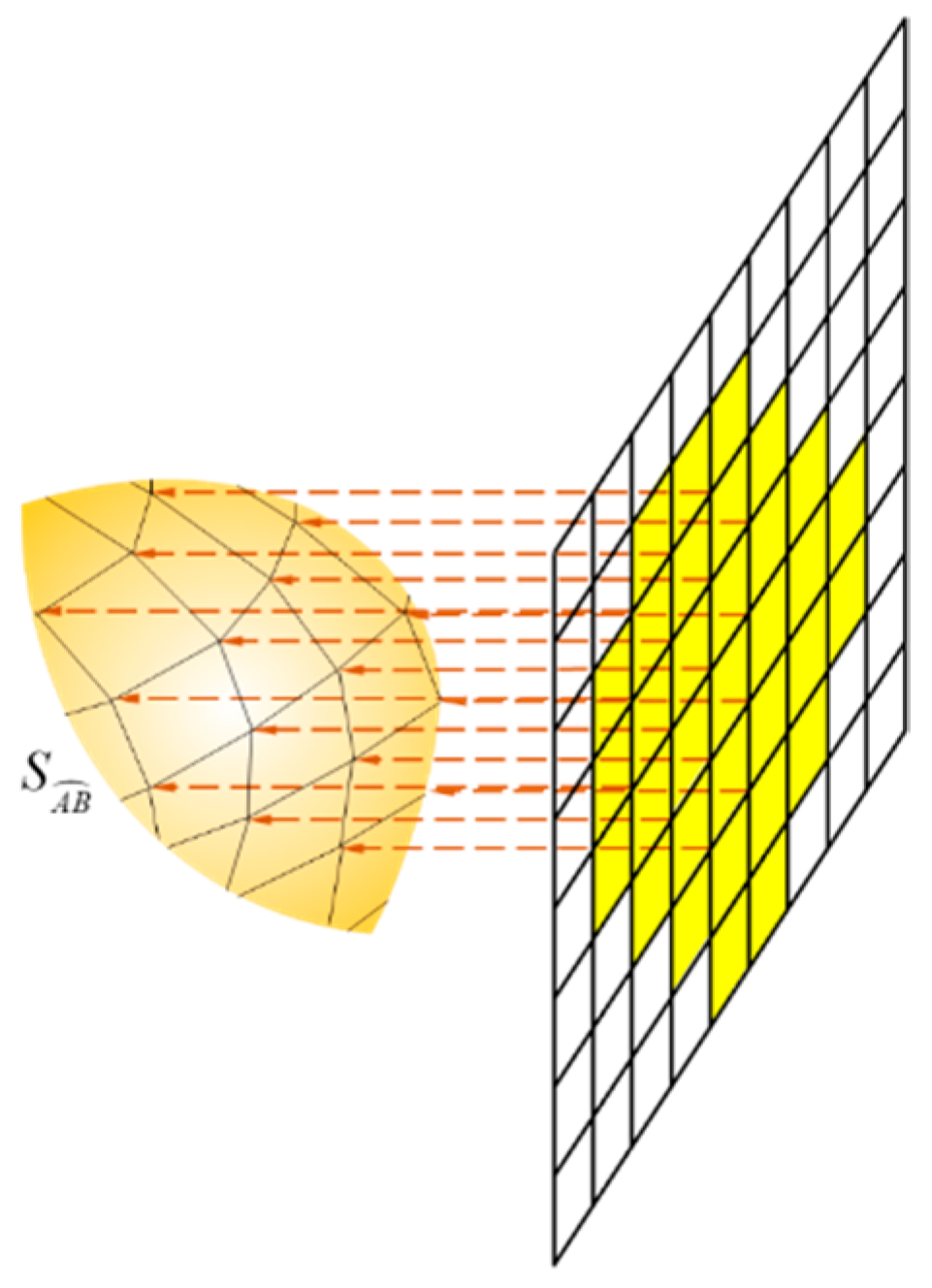
In the graphical rendering pipeline, the image of a 3D object can be projected onto a map with rectangle pixels containing the color information. Using the 3D graphical rendering technique, the target object can be discretized automatically as quadrilateral elements defined by each pixel as shown in Figure 3, and the integrating processes of each element can be implemented in the GPU thread of each pixel parallelly. Thus, the time cost of solving the backscattering of a target surface is drastically reduced.

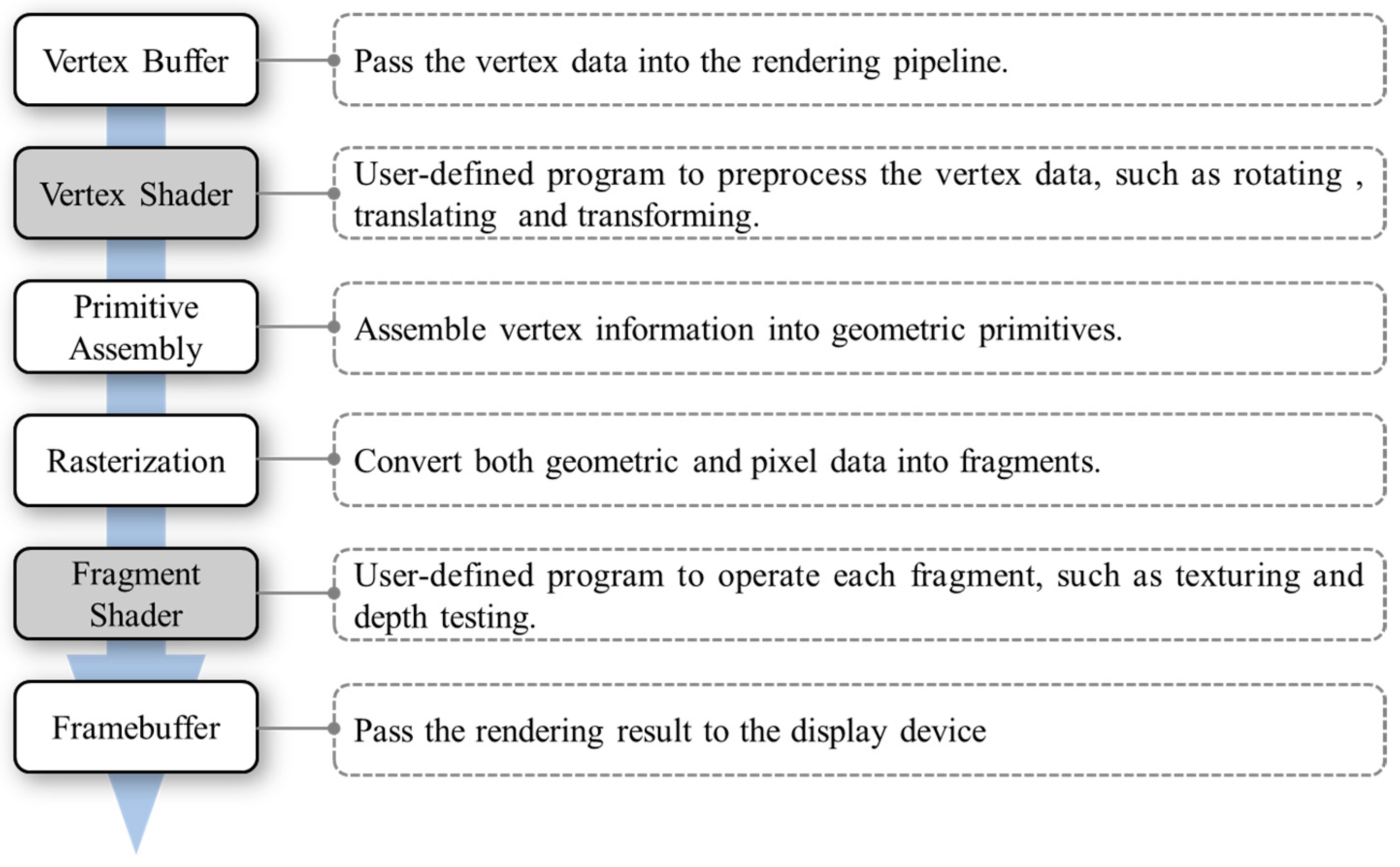
The graphical rendering pipeline of OpenGL roughly obeys the workflow in Figure 4. In the GRACO application, as the vertex shader and fragment shader are user-defined programs, the general-purpose (not just used for the graphical rendering purpose) operations can be defined in these procedures. And in the rasterization step, the 3D geometry is scanned parallelly by rays shot from each pixel, and the surface meshes are automatically generated in this step.

According to Equation (12), it can be seen that the integral results between different elements are independent of each other. Therefore, the integral procedure of each element can be processed parallelly. As shown in Figure 3, an object is insonified by an acoustic wave. And the incident acoustic wave can be approximated as a plane wave since it is emitted by a far-field source. In GRACO, the target object can be regarded as the object for rendering. The incident wave can be regarded as a group of rays perpendicular to the screen. The acoustic rays can be split into tubes by the grids defined by the screen pixels. The acoustic ray tubes cast onto the target surface generate a series of quadrilateral elements. Thus, the discretization scheme of GRACO is formed through this routine.

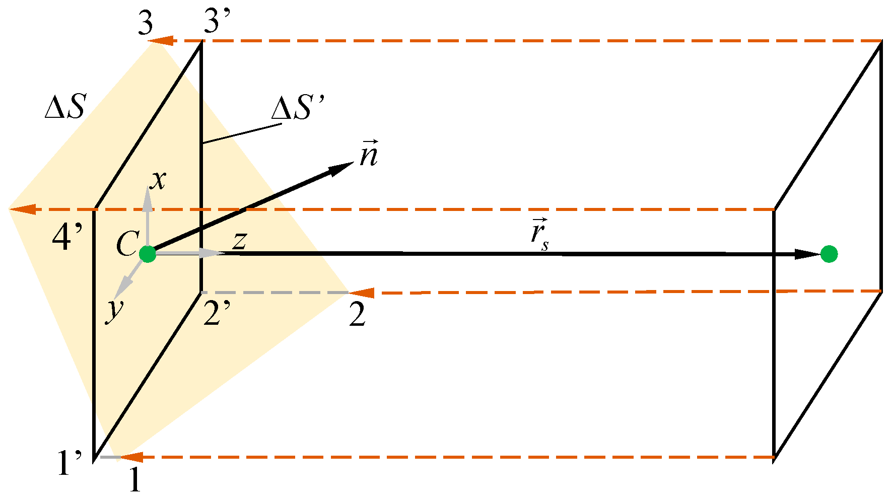
As shown in Figure 5, a single element and corresponding ray tube are extracted from the discretized model to discuss the acoustic integration of a single element. Equation (12) is still applicable for quadrilateral elements. The integral area ∆S can be projected onto the plane that is parallel to the screen plane and pass through the center point of ∆S. And Equation (12) can be transformed as

$$\mathsf{\Delta }I=e^{2ik{r}_{\mathsf{\Delta }S}}{\displaystyle \underset{\mathsf{\Delta }{S}^{\prime }}{\iint }{e}^{-2ik\overrightarrow{r}\cdot \frac{{\overrightarrow{r}}_{\mathsf{\Delta }S}}{r_{\mathsf{\Delta }S}}}V\left(\theta \right)\mathrm{d}{S}^{\prime }},$$

(14)

where $\mathrm{d}{S}^{\prime }=\mathrm{d}S\cos \theta$. In the local coordinate system of $\mathsf{\Delta }{S}^{\prime }$, the vector of normal direction is $\overrightarrow{n}=n_x\overrightarrow{i}+n_y\overrightarrow{j}+n_z\overrightarrow{k}$ and, thus, the expression of ∆S plane can be expressed as

$$n_{x}x+n_{y}y+n_{z}z=0.$$

(15)

Therefore, the integration point on ∆S can be expressed with x and y:

$$\overrightarrow{r}=\left(x,y,-\frac{n_x}{n_z}x-\frac{n_y}{n_z}y\right).$$

(16)

As the unit vector of the scattering direction is perpendicular to the screen plane, ${\overrightarrow{r}}_s/r_s=\overrightarrow{k}$. The integration of a single element can be solved:

$$\begin{array}{ll}\mathsf{\Delta }I& =e^{2ik{r}_{\mathsf{\Delta }S}}{\displaystyle \underset{\mathsf{\Delta }{S}^{\prime }}{\iint }{e}^{2ik\left(\frac{n_x}{n_z}x+\frac{n_y}{n_z}y\right)}V\left(\theta \right)\mathrm{d}x\mathrm{d}y}\\ & =e^{2ik{r}_{\mathsf{\Delta }S}}V\left(\theta \right)\left({\displaystyle {\int }_{-X/2}^{X/2}{e}^{2ik\frac{n_x}{n_z}x}\mathrm{d}x}\right)\left({\displaystyle {\int }_{-Y/2}^{Y/2}{e}^{2ik\frac{n_y}{n_z}y}\mathrm{dy}}\right)\\ & =e^{2ik{r}_{\mathsf{\Delta }S}}V\left(\theta \right)\frac{\sin \left(kX{n}_x/n_z\right)}{k{n}_x/n_z}\frac{\sin \left(kY{n}_y/n_z\right)}{k{n}_y/n_z}.\end{array}$$

(17)

where X and Y represent the dimensions of the pixel.

Embedding Equation (17) in the per-fragment shader program, the integration procedure of each element can be completed in the kernel for each pixel’s rendering. Such a solution procedure, referred to as the graphical acoustic computing method in this paper, can be carried out parallelly by a GPU and, thus, this method considerably reduces the time cost of computation [26].

2.3. The Hidden Surface Elimination Operation

In engineering practice, the target objects are usually complex. As only the illuminated regions are considered in physical optics, the shadowed surfaces should be removed when treating complex objects in the KA, and this procedure is termed the hidden surface elimination operation.

2.3.1. The Traditional Hidden Surface Elimination Technique

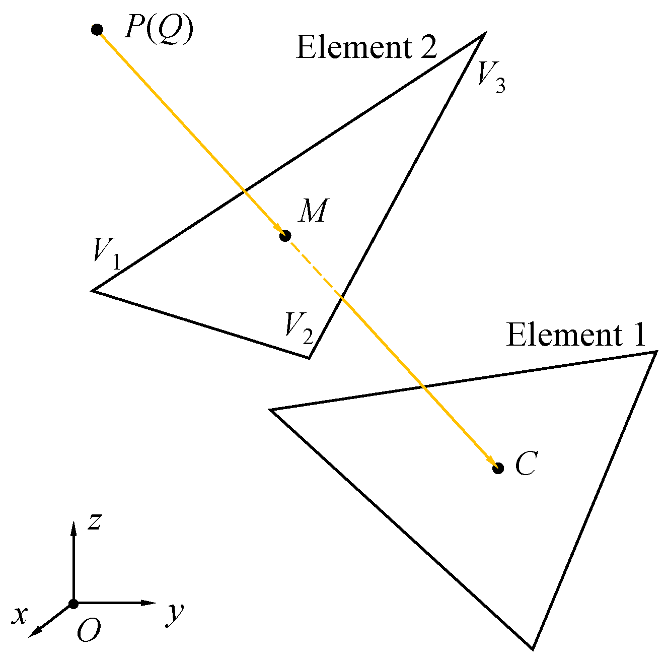
In the planar element method, there is a simple hidden surface elimination operation method performed by searching shadowed elements one by one. As shown in Figure 6, the searching procedure of this hidden surface elimination operation is organized as follows:

(1) Calculate the coordinate of M;

(2) Evaluate whether Point M is within Element 2 through Equation (18):

$$\left(\overrightarrow{V_{1}M}\times \overrightarrow{V_1{V}_2}\right)\cdot \left(\overrightarrow{V_{2}M}\times \overrightarrow{V_2{V}_3}\right)>0.$$

(18)

If Equation (18) is true, M is within Element 2 and Element 1 is regarded as shielded by Element 2; otherwise, M is out of or on the edge of Element 2 and Element 1 is not shadowed by Element 2;

(3) Repeat Step 2 until Element 2 is found to block the ray from P to C. If a shielding element for Element 1 is found, discard the integration contribution of Element 1.

This method searches shadowed elements (one by one) and each element pair through the other elements to evaluate the illumination situation of the concerned element. Thus, there are N × N instances of shadowing test time consumptions where N is the number of elements. The time cost for this method upsurges drastically with an increase in the number of elements.

2.3.2. The Z-Buffer Rendering Technique

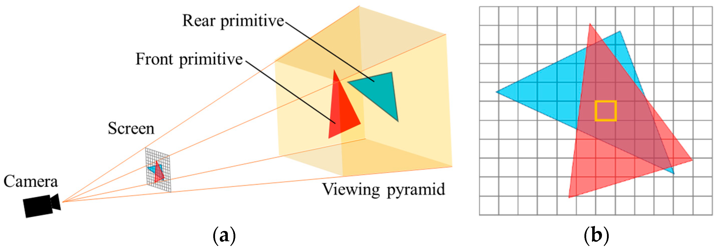
In graphical rendering, the hidden surface elimination algorithm is carried out in the rasterization step via the Z-buffer technique [38]. As shown in Figure 7a, two primitives are located in the viewing pyramid. When observing these two primitives from the position of the camera, parts of the rear primitive (blue) are shadowed by the front one (red). In OpenGL, the Z-buffer technique is applied to calculate the shadowing relationship. In the vertex shader step, the vertex coordinates of the primitives in the viewing pyramid are projected onto the screen using the MVP matrix (model, view, and projection matrix) as shown in Figure 7b. And the vertex coordinates as well as some accessory information, such as the depth, normal direction, color and texture coordinates, etc., are wrapped in the vertex data structure. In the rasterization step, each primitive is divided by the pixels as fragments. The coordinates and accessory information of each fragment are interpolated according to vertex information. For the pixels covered by more than one fragment, the depth information (the distance from the fragment to the camera) of these fragments is compared, and the nearest fragment is chosen to render the current pixel.

During the OpenGL rendering procedures, the projection, scanning, interpolation, and comparison of operations are implemented parallelly in the GPU kernels. Thus, the time cost of hidden surface elimination operations is drastically cut by the parallel program, compared to the traditional hidden surface elimination technique.

2.4. The Depth Peeling and Scattering of Multiple-Layered Structures for GRACO

In the previous sections, only the acoustic backscattering of the outermost surface is considered. That is, the backscattering wave is composed of reflecting waves from the outmost surface but no acoustic wave penetrates through the outer surface and strikes the inner structure. When considering the acoustic backscattering contribution of the inner structure, there are two extra aspects needed to be considered: (1) the transmission coefficient penetrating the outer surfaces should be defined; (2) how to identify shadowing element pairs.

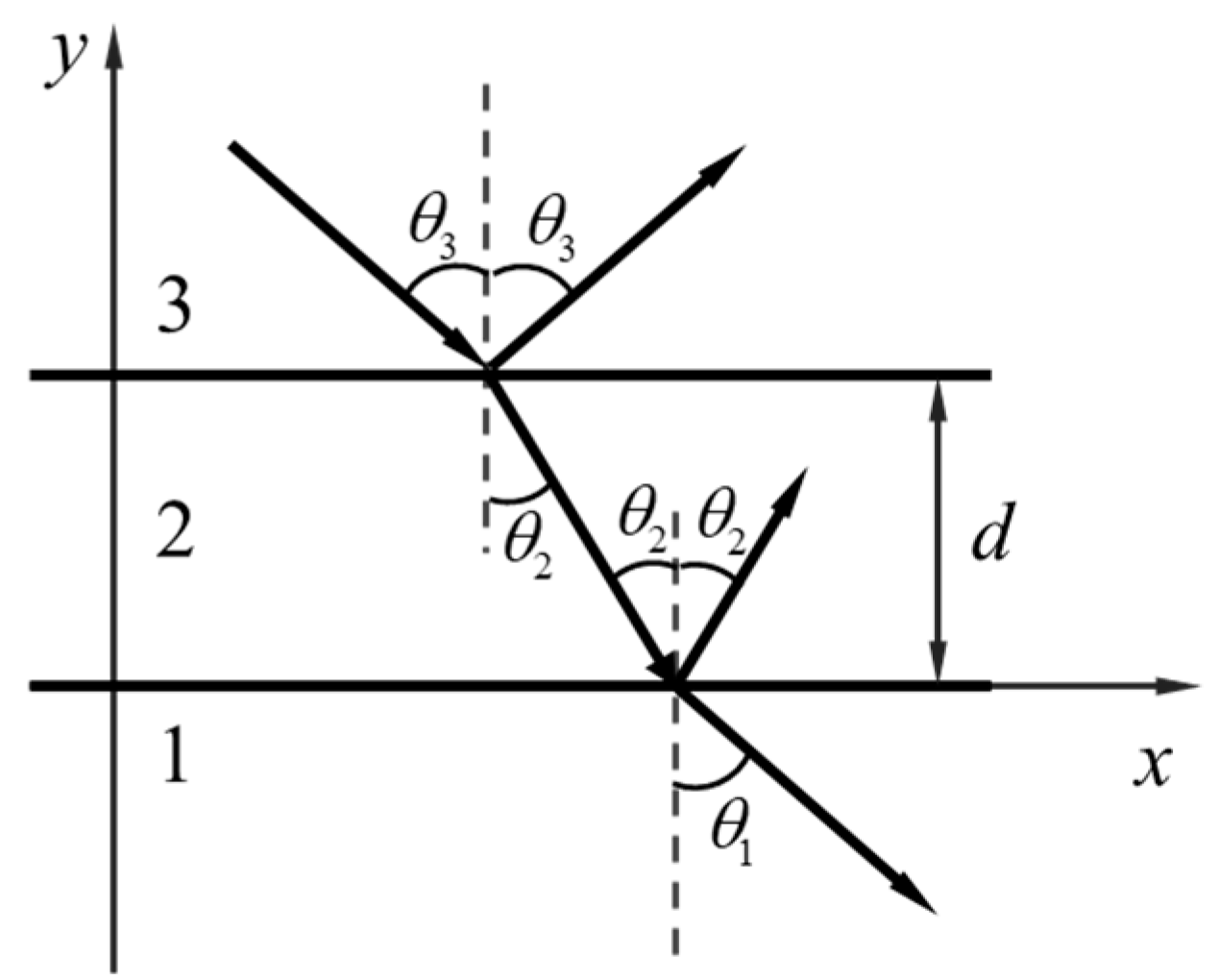
Due to the properties of the target elements being regarded as those of an infinite tangent plane in the Kirchhoff approximation, the reflection and transmission coefficients can be approximated with those of an infinite plane. According to waves in layered media [39], the reflection and transmission coefficients of an infinite plane as shown in Figure 8 are

$$V=\frac{\left(Z_1+Z_2\right)\left(Z_2-Z_3\right)e^{-\mathrm{i}{k}_{2z}d}+\left(Z_1-Z_2\right)\left(Z_2+Z_3\right)e^{\mathrm{i}{k}_{2z}d}}{\left(Z_1+Z_2\right)\left(Z_2+Z_3\right)e^{-\mathrm{i}{k}_{2z}d}+\left(Z_1-Z_2\right)\left(Z_2-Z_3\right)e^{\mathrm{i}{k}_{2z}d}},$$

(19)

and

$$W=\frac{1+V}{\cos \left(k_{2z}d\right)-\mathrm{i}\left(Z_2/Z_1\right)\sin \left(k_{2z}d\right)}$$

(20)

where k_2z is the z-directional component of the second-layer wave vector, d is the thickness of the second layer, and Z_i is the acoustic impedance of the ith layer medium.

$$Z_i=\frac{{\rho }_i{c}_i}{\cos {\theta }_i},i=1,2,3,$$

(21)

where ρ_i and c_i are the density and acoustic velocity of ith layer, respectively.

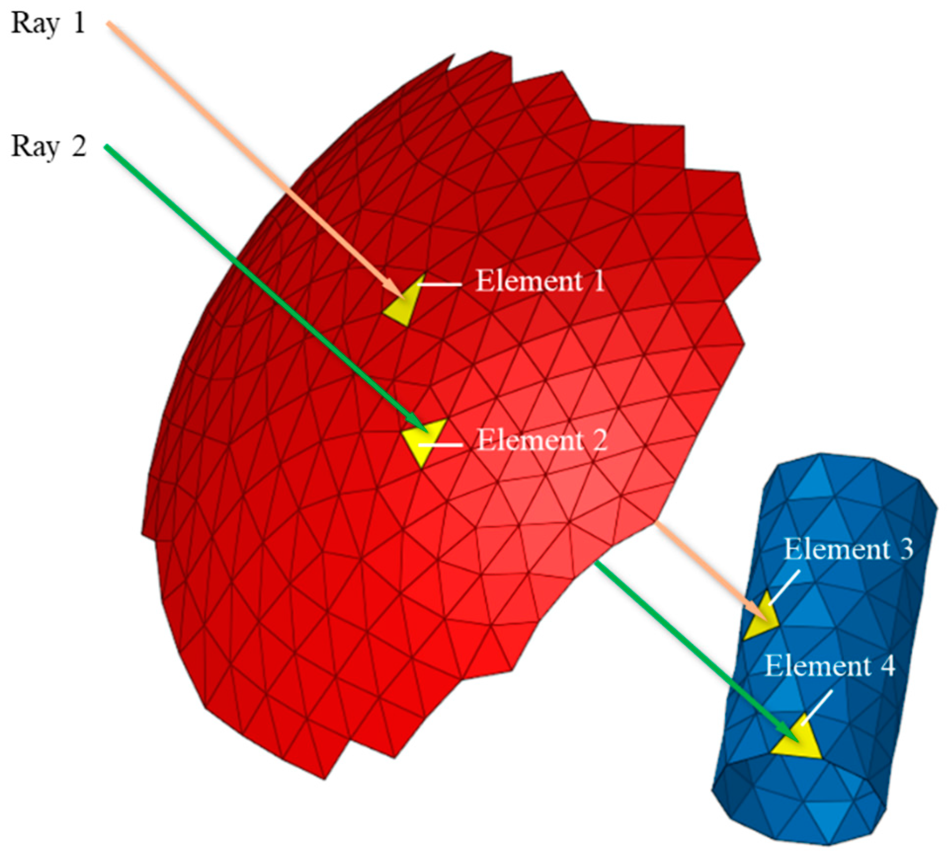
As shown in Figure 9, the acoustic rays insonify a complex target with an outer surface (red) and an inner structure (blue). If the outer surface is acoustic-penetrable, the existence of the inner structure makes contributions to the total backscattering. Due to the incident angle being different, the transmission coefficients of Element 1 and 2 shot by parallel rays are different. Thus, the weight coefficients for the contributions of each inner element (Elements 3 and 4) are not always the same. The weight coefficients for inner elements are determined by the outer-layer elements that shield each inner element from incident acoustic rays. That is, the weight coefficient of Element 3 is determined by the transmission coefficient of Element 1 and Element 4 is determined by Element 2. Therefore, an algorithm for identifying the shadowing element pairs between the outer surface and the inner structure is needed to designate proper weight coefficients for inner elements.

In the traditional discretized KA, the technique of finding shadowing pairs is the same as that in the traditional hidden surface elimination technique. Similarly, the shadow test operations are carried out element by element for each considered element, and this method is quite inefficient.

In 3D graphical rendering, the depth peeling (DP) method which is commonly applied to render semi-transparent materials can be utilized to consider the penetration of the acoustic rays. In the previous section, the Z-buffer technique is introduced to select the fragments nearest to the camera at each pixel. In the depth peeling method, the target object is rendered multiple times, and the rendering results are stored in different layers of framebuffers. For the first layer, the fragments nearest to the camera at each pixel are rasterized and stored in the first-layer framebuffer. For the second layer, at each pixel, the fragments whose Z-depth values are smaller than that in the first-layer framebuffer at the current pixel are discarded, and the fragments which are second nearest to the camera are rendered and stored in the second-layer framebuffer. For higher-order layers, the depth values of the previous layer are taken as the threshold to filter out the fragments that have been rendered in the previous layers. After rendering the images of different layers, the framebuffers in different layers are blended with weighted coefficients, and the image of the semi-transparent object is acquired.

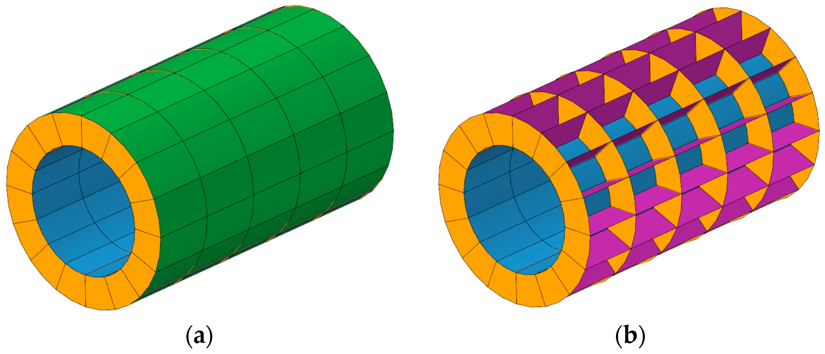
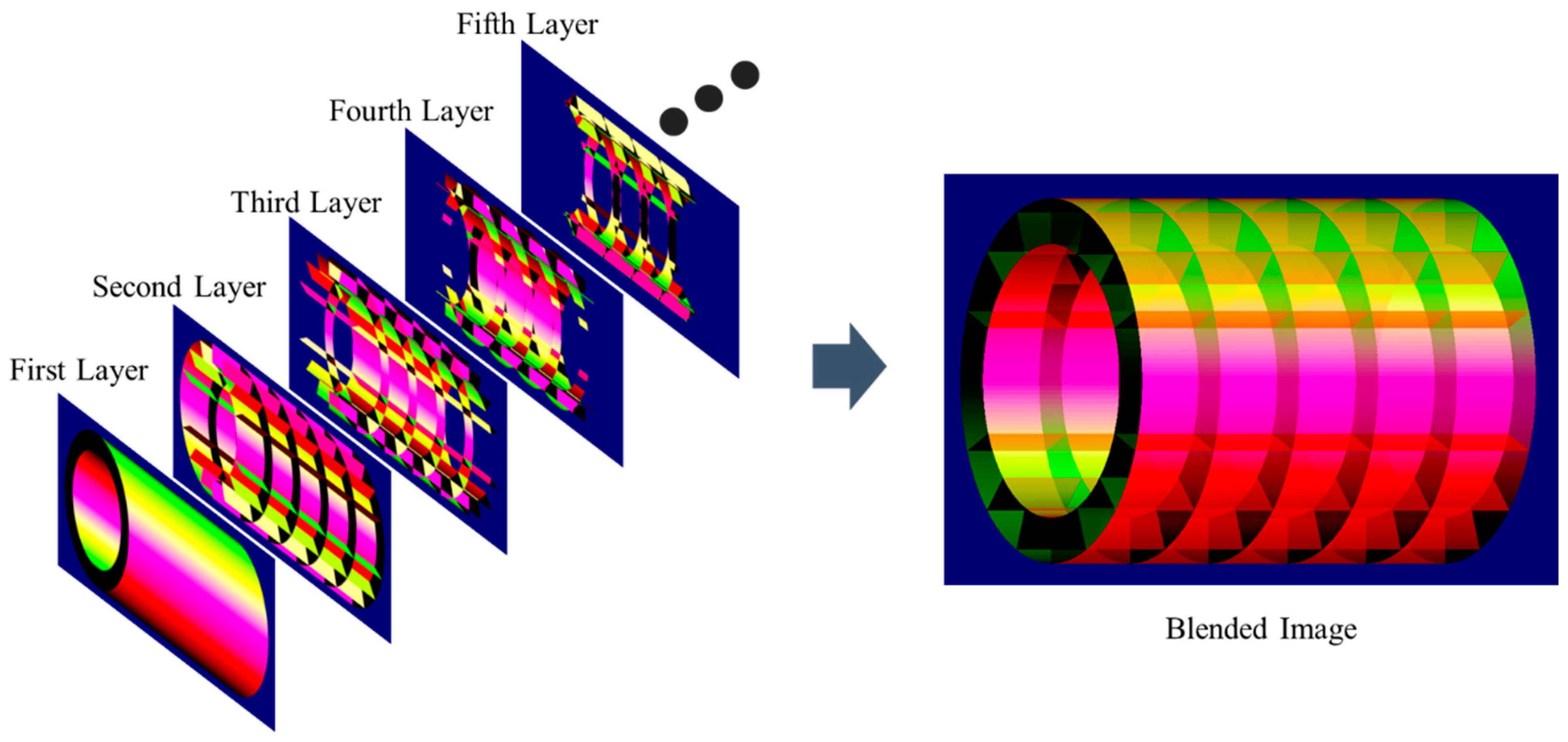
An example double shell with grids is presented in Figure 10. As shown in Figure 11, the depth peeling method is used to render this semi-transparent double shell. In this depth peeling rendering pipeline, the color of each pixel is defined as the normal direction of each rendered element. The fragments that are first nearest, second nearest, third nearest, etc., are projected onto the pixels of first-layer, second-layer, third-layer, etc., framebuffers. After the rendering of different layers, the target semi-transparent image is acquired by blending the image of different layers together.

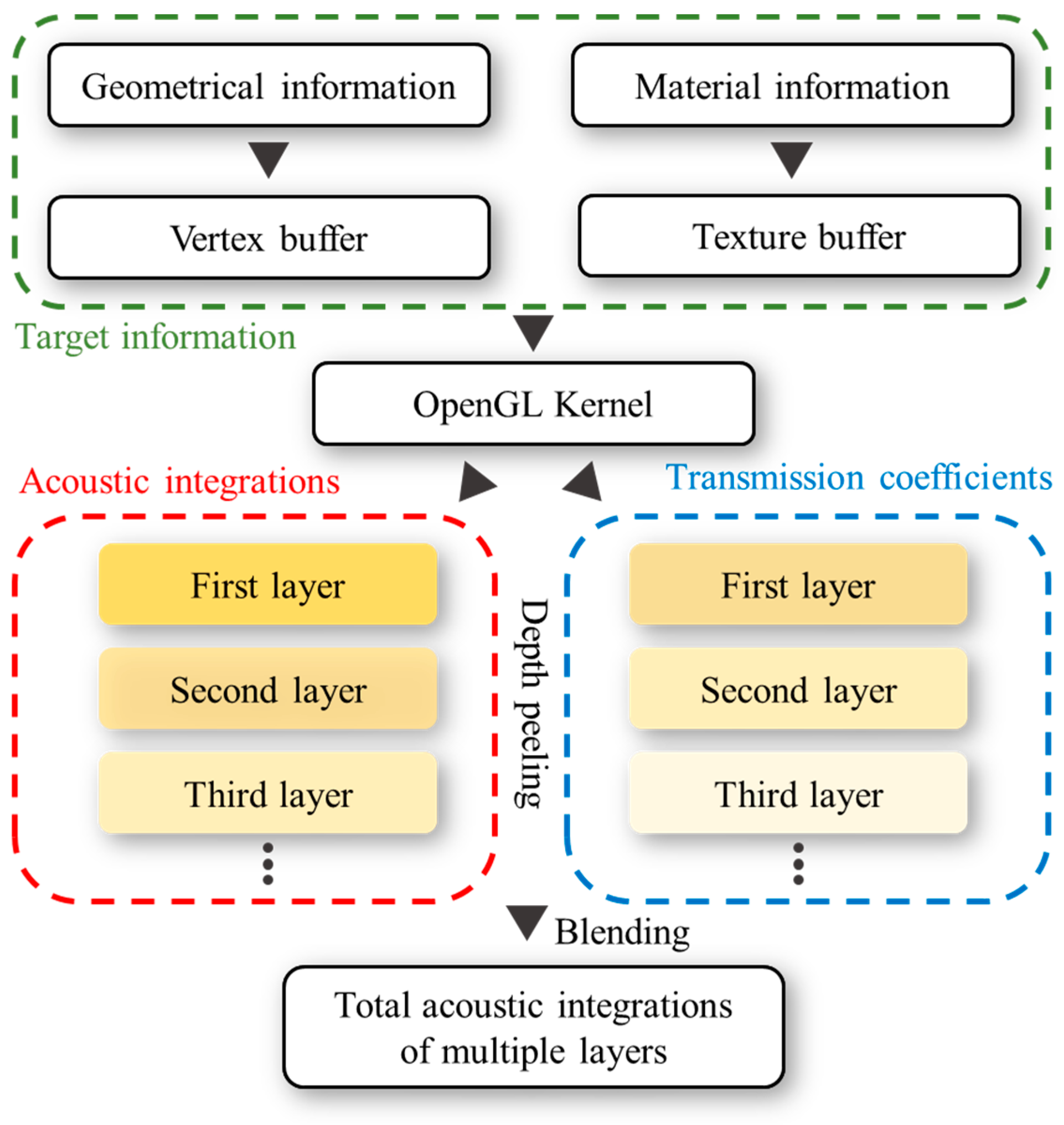
In GRACO, the depth peeling technique can be applied to cope with the penetration of acoustic rays. As shown by the procedures in Figure 12, both the backscattering integrations and transmission coefficients of the nearest nth layer are rendered through the depth peeling technique, and then, the total backscattering contributions of the outer surface as well as the internal structure can be acquired through summing up the integration results of different layers weighted with the previous layer’s transmission coefficient:

$$\mathsf{\Delta }{I}_{\mathrm{total}}=\mathsf{\Delta }{I}_1+{\displaystyle \sum _{i=2}^N\left[\left({\displaystyle \prod _{j=1}^{i-1}{W}_j^2}\right)\mathsf{\Delta }{I}_i\right]},$$

(22)

where $\mathsf{\Delta }{I}_1$ is the acoustic integration of the ith-layer element, and $W_j$ is the transmission coefficient of the jth-layer element.

3. Examples and Discussions

3.1. GRACO Solutions for Typical Models

3.1.1. A Sphere Model

An impedance sphere with 1 m radius is insonified by an acoustic source point whose velocity potential is ${\varphi }_i\left(\overrightarrow{r}\right)=\frac{e^{ik\left|{\overrightarrow{r}}_P-\overrightarrow{r}\right|}}{r_P}$. As the source point is far from the sphere, the acoustic field near the sphere can be regarded as a plane wave as shown in Figure 13. Setting the sphere center O as the origin point and the direction from P to O as the x axis, the velocity potential of the incident wave near the sphere can be approximated as

$${\varphi }_i\left(\overrightarrow{r}\right)=A{e}^{ikx},A=\frac{e^{ik{r}_P}}{r_P}.$$

(23)

According to the PWS solution, the backscattering of the impedance sphere in a plane wave can be expressed as [2]

$$\{\begin{array}{l}{\varphi }_s\left(r,\theta \right)=-A{\displaystyle \sum _{n=0}^{\infty }{\mathrm{i}}^n\left(2n+1\right)b_n\left(ka\right)h_n^{\left(1\right)}\left(kr\right)P_n\left(\cos \theta \right),}\\ b_n\left(ka\right)=\frac{j_n{}^{\prime }\left(ka\right)+\mathrm{i}\beta j_n\left(ka\right)}{h_n^{\left(1\right){}^{\prime }}\left(ka\right)+\mathrm{i}\beta h_n^{\left(1\right)}\left(ka\right)},\\ \beta =\frac{\rho c}{Z}.\end{array}$$

(24)

where $j_n(\cdot )$ is the spherical Bessel function, $h_n^{\left(1\right)}(\cdot )$ is the spherical Hankel function of the first kind, $P_n(\cdot )$ is the Legendre function, and β is the specific admittance of the surface.

Referenced by the PWS solution, the target strength of this model is also given by other numerical and asymptotic methods: FEM, BEM, PEM, and GRACO. The solution schemes of PEM and GRACO are given in Equation (13) and Equation (17), respectively. The hardware and software used in different methods are listed in

Table 1. The hardware and software used in different methods.

	PWS/PEM	FEM/BEM	GRACO
Hardware	CPU: Intel (R) Xeon (R) CPU E5-2643 v4 @ 3.4 GHz RAM: 128 GB GPU: NVIDIA Quadro M4000
Software	Matlab2020a	COMOSOL 5.6	Visual Studio 2017

. The TSs of the sphere with different normal absorbing coefficients solved by different methods are presented in Figure 14. And the time costs of different methods for different models are listed in

Table 2. Time costs for different methods.

Frequency f (Hz)	Element Size Δ (m)	Time Costs t (s)
		FEM	BEM	PEM	GRACO
1000	0.25	12	7	0.019	0.031
2000	0.125	65	20	0.042	0.030
3000	0.083	289	48	0.117	0.030
4000	0.063	865	83	0.263	0.034
5000	0.05	5825	142	0.543	0.033

Note: The pixel number used in GRACO is fixed to N_pixel = 1000 × 1000 for different models, and the size of the screen is mapped to 2 m × 2 m, i.e., the pixel dimensions for the current models of GRACO are set to X = 0.002 m and Y = 0.002 m.

.

As can be seen from Figure 14, the solutions of FEM and BEM almost coincide with the analytical PWS solution, while the overlapping KA and GRACO solutions fluctuate around the PWS solution. The cause of the different accuracies between FEM/BEM and KA/GRACO is that both FEM and BEM are based on the rigorous model and the solutions of these methods are sufficiently accurate when appropriately dense meshes are selected, while the contribution of the shadowed areas of the target are omitted for both KA and GRACO and the solutions of these methods cannot match well with the analytical solution, especially in the low-frequency range (i.e., ka < 2π, where a is the half of the major size of projection of the scatterer).

Although the accuracy of GRACO cannot compete with that of some rigorous numerical methods like FEM and BEM, GRACO is still prioritized in engineering practice when considering large objects in high-frequency ranges. The reason for GRACO’s priority is due to the time costs of FEM and BEM as shown in Table 1. For the current example at f = 5000 Hz, the time cost is about 5825 s for the FEM model, 142 s for BEM, 0.543 s for PEM, and 0.033 s for GRACO. For larger objects or higher frequencies, the time costs of FEM and BEM are intolerable.

3.1.2. A BeTSSi Benchmark Submarine

In this section, the target strengths of a BeTTSi [40] submarine (Benchmark Target Echo Strength Simulation) with different normal absorption coefficients are considered by both GRACO and BEM. The major dimensions of the considered submarine model are total length L = 62 m and radius of the body r = 3.5 m. The pixel dimensions for the current model of GRACO are set to X = 0.02 m and Y = 0.02 m. The figure of this submarine is illustrated in Figure 15. The target predictions of such a model are presented in Figure 16.

Since there is no analytical solution for this benchmark model, the BEM solution is chosen as the reference solution instead. Considering the massive time and calculation resource consumption, the frequency of the incident wave is controlled within relatively low values, i.e., f = 500 Hz and 1000 Hz. According to Figure 16, it can be figured out that the TS curves predicted by GRACO are quite close to the reference solutions predicted by BEM at most incident directions. At the incident direction in the vicinity of θ = 0° and 180°, there are visible errors in the GRACO solution. This is because the ka values of such cases are smaller than those in cases with incident angle θ = 90°. The differences between GRACO and BEM at θ = 0° and 180° in Figure 16a,b are much bigger than those in Figure 16c,d. It can be deduced that the error of GRACO is negatively correlated to this ka value.

According to the examples of the sphere and benchmark models, it can be recognized that KA-based GRACO is a sufficiently accurate method for the TS prediction of high-frequency acoustic backscattering. Especially, in most engineering application practices, time and economic issues usually draw more concern than accuracy. Therefore, GRACO harbors more advantages than rigorous numerical methods, such as FEM and BEM.

3.2. Comparison of GRACO and GRACO–DP

3.2.1. A Pair of Circular Plates

Most underwater vehicles are multiple-layered structures. There are always inner shells, platforms, ribs, etc., inside the outmost surface. It is necessary to investigate the acoustic backscattering contribution of inner structures. In this section, a pair of circular plates is taken as the example as shown in Figure 17. This pair of plates is made of steel with Young’s modulus E = 210 GPa and Poisson’s ratio ν = 0.3. The target strength of this model is calculated with three different methods: FEM, GRACO, and GRACO–DP. The pixel dimensions for the current model of GRACO are set to X = 0.002 m and Y = 0.002 m. The results are presented in Figure 18.

In Figure 18, the target strength of the pair of circular plates is predicted through three different methods. FEM is verified as sufficiently precise and, thus, it is regarded as the reference method in the current example. Both GRACO and GRACO–DP are based on high-frequency Kirchhoff approximations. The difference between these two methods is that GRACO only considers the backscattering contribution of the elements nearest to the observer, while GRACO–DP can collect the acoustic backscattering contribution of inner structures through the depth peeling technique. It can be determined from Figure 18a,b that the solution determined by GRACO–DP can fit better than that of GRACO to the FEM solution. It can also be found that the solutions of both FEM and GRACO–DP reach a bottom value at f = 3200 Hz while the solution of GRACO does not fall at this point. To explain this phenomenon, the phase differences between the outermost surface and the shadowed area are obtained and illustrated in Figure 19, where φ_near is the phase of the backscattering velocity potential of the directly illuminated elements and φ_far is the phase of the backscattering velocity potential of the shadowed elements. Figure 19 demonstrates that the phase difference φ_far-φ_near reaches 180° at f = 3200 Hz. Thus, the backscattering of the shadowed area counteracts parts of the backscattering contribution of the directly illuminated area. And these counteracting effects lead to the falling point at f = 3200 Hz of FEM and GRACO–DP, while the traditional GRACO method cannot take this part into account.

3.2.2. A Ribbed Double Shell

In this section, a ribbed double shell is constructed and its measurements are given as shown in Figure 20. The outer and inner diameters of the shell are 4 m and 3 m, respectively. The length of the shell is 6 m. Four longitudinal trusses are circumferentially distributed and six transverse ribs are arranged evenly along the length direction. The walls and ribs of the structure are made of 5 mm steel with Young’s modulus E = 210 GPa and Poisson’s ratio ν = 0.3. Water is present between the outer and inner shells. The target strengths of this model are solved by both GRACO and GRACO–DP. The pixel dimensions for the current model of GRACO are set to X = 0.002 m and Y = 0.002 m. TS maps altering with the incident angle θ and the frequency f are presented in Figure 21. Additionally, the TS–θ curves at f = 2000, 5000, 8000, and 10,000 Hz are extracted and depicted in Figure 22.

As shown in Figure 21 and Figure 22, the target strength predicted by GRACO–DP is much larger than that predicted by GRACO. According to Figure 21b, acquired from GRACO–DP, there are some pairs of “/\-shaped” bright trending lines, whereas these trending lines cannot be spotted in Figure 21a which was acquired from GRACO. These bright trending lines are Bragg waves [41] generated by the periodically arranged ribs covered by the outer surface. These phenomena mean the backscattering contributions of the inner structures are considerable compared to the total backscattering.

4. Conclusions

In this work, a KA-based GRACO method is introduced to deal with high-frequency acoustic backscattering problems of large-scale objects. Also, the depth peeling technique which is commonly used to deal with the 3D graphical rendering of transparent objects is integrated into the GRACO method to consider the backscattering contributions of inner structures. Some numerical examples are carried out with the following conclusions:

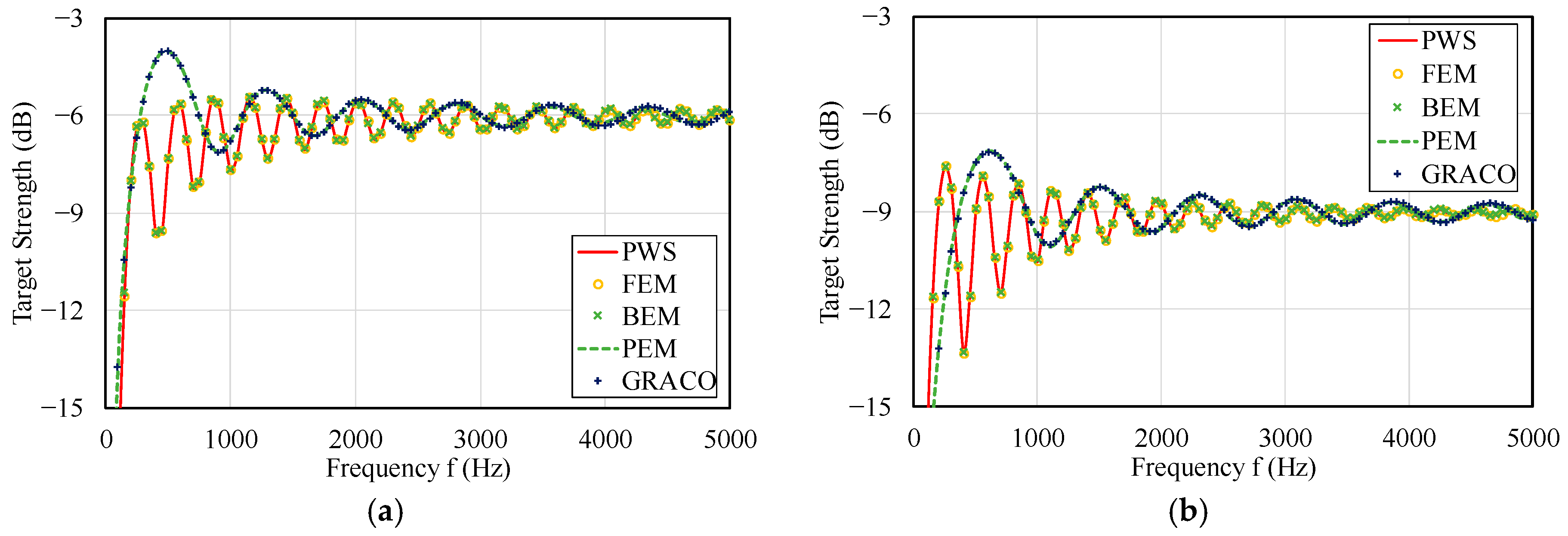
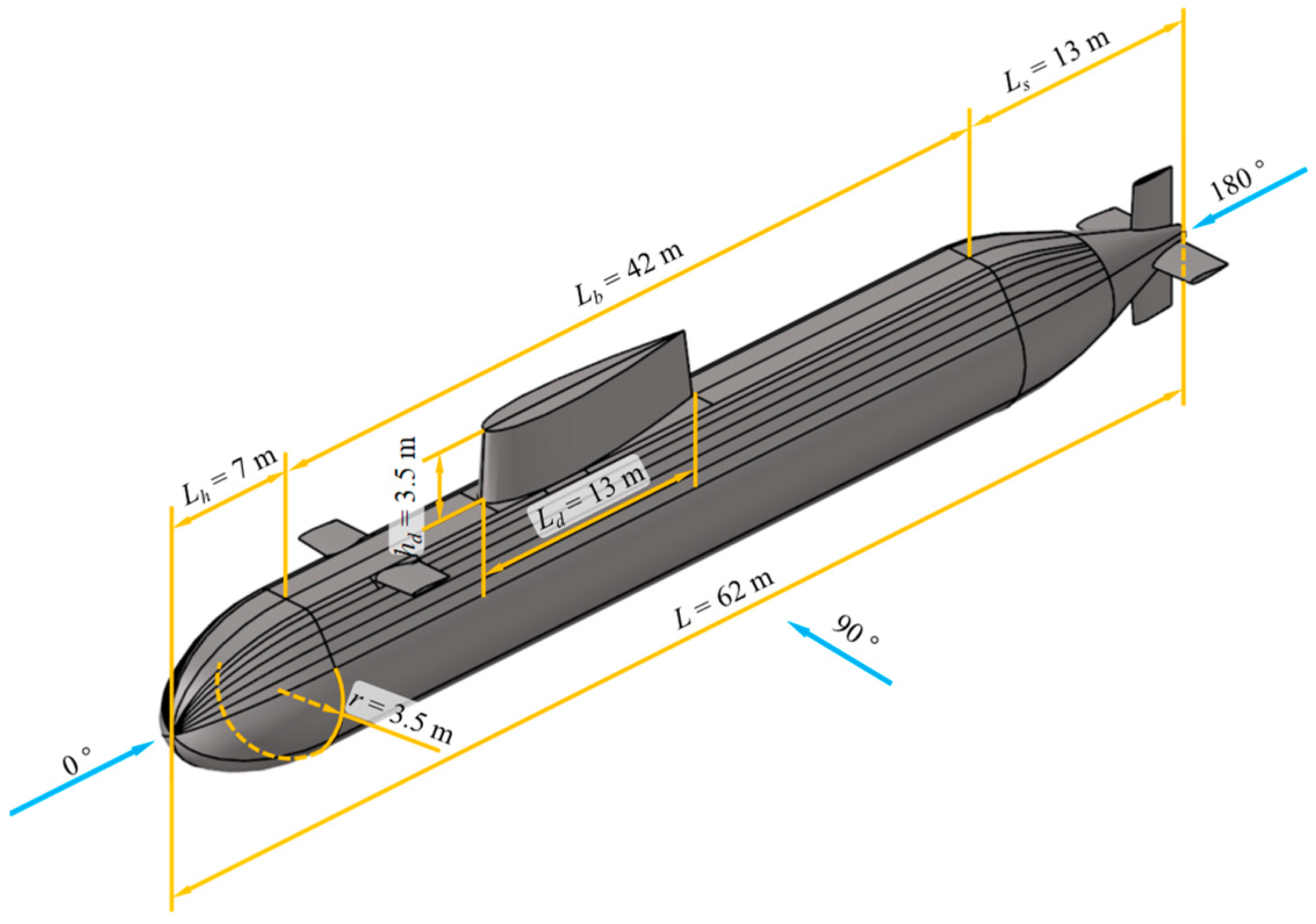
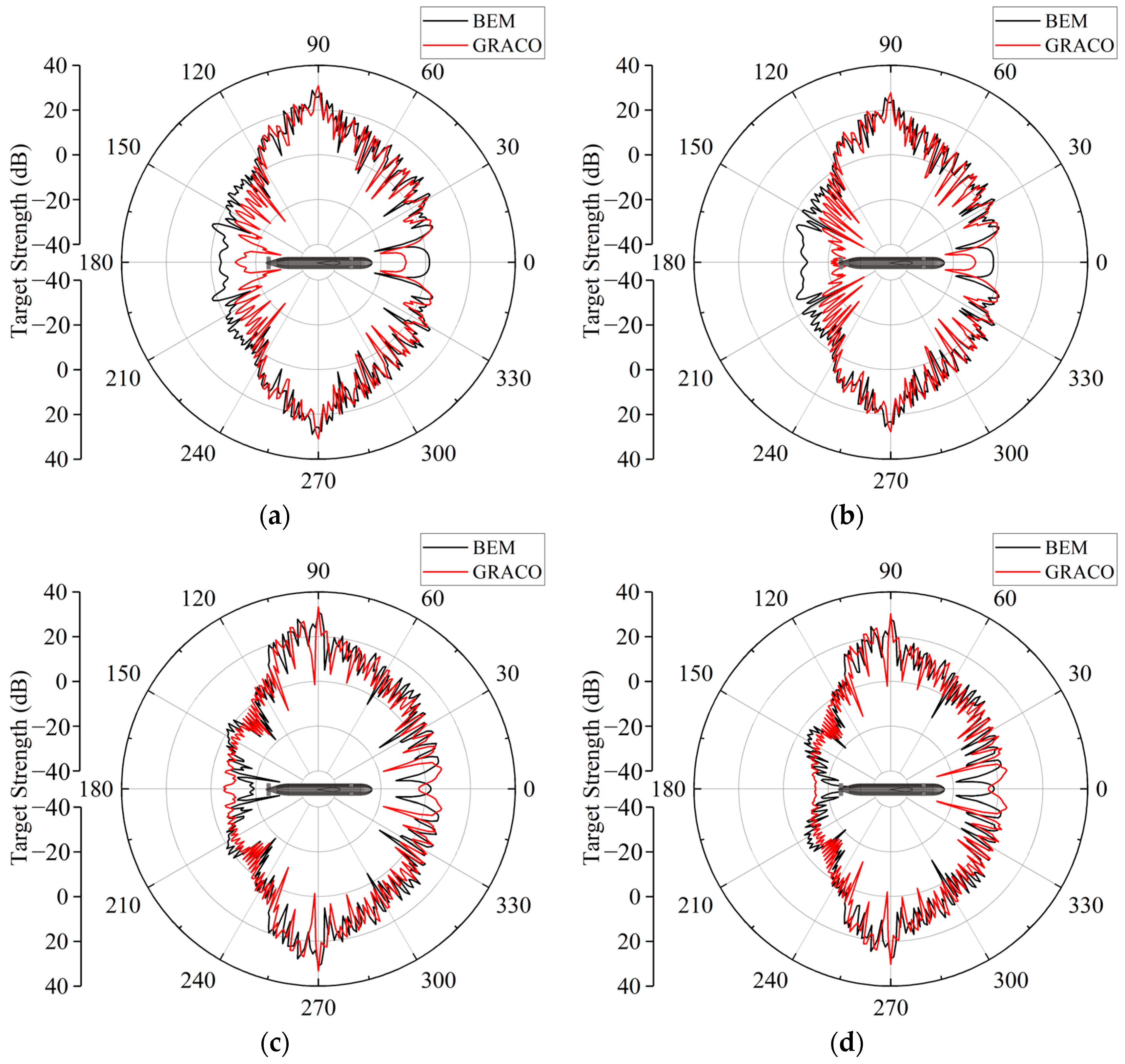
Firstly, the target strength of an impedance sphere and a large-scale benchmark model has been evaluated with different methods. Through the solutions of the sphere example, it can be determined that the GRACO method can acquire sufficient accurate TS solutions for high-frequency backscattering problems with much less computational consumption and time costs. The numerical example of the benchmark model tells one that GRACO performs well in terms of accuracy when predicting the target strength of complex object and that GRACO still keeps high efficiency when coping with the high-frequency backscattering of large-scale models while traditional numerical methods like FEM and BEM have difficulties concerning efficiency and computational costs.

Secondly, a pair of circular plates is taken as an example to discuss the backscattering of multiple-layer structures. Compared to the traditional GRACO method, the GRACO–DP method can properly obtain the backscattering contributions that are shadowed by outer surfaces. Therefore, the solution of GRACO–DP is better fitted to the FEM solution which is regarded as the reference solution of this example.

Finally, a ribbed double shell model is considered by both the GRACO and GRACO–DP. The results show that there exist considerable differences between the solutions from different methods for most incident angles. Moreover, features of Bragg waves which are generated by the periodically arranged ribs can be spotted from the GRACO–DP solution, while such features cannot be observed from the solution of GRACO. Thus, in engineering practice, the combination of DP and GRACO is necessary for determining the backscattering of multiple-layered structures.

The current work shines light on the backscattering correction of a KA-based method considering the acoustic penetration of multiple-layered structures, but some limitations and problems remain unresolved and need to be studied in future works. For example, the multiple back-and-forth reflections between the outer surfaces and the inner shells should be considered more carefully. Furthermore, the influence of the curvature of the surfaces on the transmission coefficients is not discussed in detail.

References

1. Rayleigh, J.W.S.B. The Theory of Sound; Macmillan & Company: London, UK, 1896. [Google Scholar]
2. Morse, P.M.C. Vibration and Sound; McGraw-Hill: New York, NY, USA, 1948. [Google Scholar]
3. Morse, P.M.C.; Ingard, K.U. Theoretical Acoustics; Princeton University Press: Princeton, NJ, USA, 1986. [Google Scholar]
4. Faran, J.J., Jr. Sound scattering by solid cylinders and spheres. J. Acoust. Soc. Am. 1951, 23, 405–418. [Google Scholar] [CrossRef]
5. Junger, M.C. Sound scattering by thin elastic shells. J. Acoust. Soc. Am. 1952, 24, 366–373. [Google Scholar] [CrossRef]
6. Stanton, T.K. Sound scattering by cylinders of finite length. I. Fluid cylinders. J. Acoust. Soc. Am. 1988, 83, 55–63. [Google Scholar] [CrossRef]
7. Stanton, T.K. Sound scattering by cylinders of finite length. II. Elastic cylinders. J. Acoust. Soc. Am. 1988, 83, 64–67. [Google Scholar] [CrossRef]
8. Stanton, T.K. Sound scattering by cylinders of finite length. III. Deformed cylinders. J. Acoust. Soc. Am. 1989, 86, 691–705. [Google Scholar] [CrossRef]
9. Waterman, P.C. New formulation of acoustic scattering. J. Acoust. Soc. Am. 1969, 45, 1417–1429. [Google Scholar] [CrossRef]
10. Waterman, P. Matrix theory of elastic wave scattering. J. Acoust. Soc. Am. 1976, 60, 567–580. [Google Scholar] [CrossRef]
11. Gong, Z.; Li, W.; Chai, Y.; Zhao, Y.; Mitri, F.G. T-matrix method for acoustical Bessel beam scattering from a rigid finite cylinder with spheroidal endcaps. Ocean. Eng. 2017, 129, 507–519. [Google Scholar] [CrossRef]
12. Gong, Z.; Li, W.; Mitri, F.G.; Chai, Y.; Zhao, Y. Arbitrary scattering of an acoustical Bessel beam by a rigid spheroid with large aspect-ratio. J. Sound Vib. 2016, 383, 233–247. [Google Scholar] [CrossRef]
13. Seybert, A.F.; Soenarko, B.; Rizzo, F.J.; Shippy, D.J. An advanced computational method for radiation and scattering of acoustic waves in three dimensions. J. Acoust. Soc. Am. 1985, 77, 362–368. [Google Scholar] [CrossRef]
14. Seybert, A.F.; Rengarajan, T.K. The use of CHIEF to obtain unique solutions for acoustic radiation using boundary integral equations. J. Acoust. Soc. Am. 1987, 81, 1299–1306. [Google Scholar] [CrossRef]
15. Hunt, J.T.; Knittel, M.R.; Barach, D. Finite element approach to acoustic radiation from elastic structures. J. Acoust. Soc. Am. 1974, 55, 269–280. [Google Scholar] [CrossRef]
16. Hunt, J.T.; Knittel, M.R.; Nichols, C.S.; Barach, D. Finite−element approach to acoustic scattering from elastic structures approach to acoustic scattering from elastic structures. J. Acoust. Soc. Am. 1975, 57, 287–299. [Google Scholar] [CrossRef]
17. Karasalo, I. Modelling of acoustic scattering from a submarine. In Proceedings of the Meetings on Acoustics, Edinburgh, UK, 2 July 2012; Volume 17, p. 070017. [Google Scholar]
18. Wilkes, D.R.; Duncan, A.J.; Marburg, S. A Parallel and Broadband Helmholtz FMBEM Model for Large-Scale Target Strength Modeling. J. Theor. Comput. Acoust. 2020, 28, 2050001. [Google Scholar] [CrossRef]
19. Chai, Y.; Li, W.; Gong, Z.; Li, T. Hybrid smoothed finite element method for two-dimensional underwater acoustic scattering problems. Ocean. Eng. 2016, 116, 129–141. [Google Scholar] [CrossRef]
20. Chai, Y.; You, X.; Li, W. Dispersion reduction for the wave propagation problems using a coupled “FE-Meshfree” triangular element. Int. J. Comput. Methods 2020, 17, 1950071. [Google Scholar] [CrossRef]
21. You, X.; Gui, Q.; Zhang, Q.; Chai, Y.; Li, W. Meshfree simulations of acoustic problems by a radial point interpolation method. Ocean. Eng. 2020, 218, 108202. [Google Scholar] [CrossRef]
22. Li, Y.; Dang, S.; Li, W.; Chai, Y. Free and forced vibration analysis of two-dimensional linear elastic solids using the finite element methods enriched by interpolation cover functions. Mathematics 2022, 10, 456. [Google Scholar] [CrossRef]
23. Gui, Q.; Zhang, G.; Chai, Y.; Li, W. A finite element method with cover functions for underwater acoustic propagation problems. Ocean. Eng. 2022, 243, 110174. [Google Scholar] [CrossRef]
24. Chai, Y.B.; Huang, K.Y.; Wang, S.P.; Xiang, Z.C.; Zhang, G.J. The Extrinsic Enriched Finite Element Method with Appropriate Enrichment Functions for the Helmholtz Equation. Mathematics 2023, 11, 1664. [Google Scholar] [CrossRef]
25. Liu, C.; Min, S.; Pang, Y.; Chai, Y. The Meshfree Radial Point Interpolation Method (RPIM) for Wave Propagation Dynamics in Non-Homogeneous Media. Mathematics 2023, 11, 523. [Google Scholar] [CrossRef]
26. Gui, Q.; Li, W.; Chai, Y.B. The enriched quadrilateral overlapping finite elements for time-harmonic acoustics. Appl. Math. Comput. 2023, 451, 128018. [Google Scholar] [CrossRef]
27. Li, Y.C.; Liu, C.; Li, W.; Chai, Y.B. Numerical investigation of the element-free Galerkin method (EFGM) with appropriate temporal discretization techniques for transient wave propagation problems. Appl. Math. Comput. 2023, 442, 127755. [Google Scholar] [CrossRef]
28. Urick, R.J. Principles of Underwater Sound Third Edition; McGraw-Hill: New York, NY, USA, 1983. [Google Scholar]
29. Kerr, D.E. Propagation of Short Radio Waves; McGraw-Hill: New York, NY, USA, 1951. [Google Scholar]
30. Gordon, W. Far-field approximations to the Kirchoff-Helmholtz representations of scattered fields. IEEE Trans. Antennas Propag. 1975, 23, 590–592. [Google Scholar] [CrossRef]
31. Fan, J.; Tang, W.L.; Zhuo, L.K. Planar elements method for forecasting the echo characteristics from sonar targets. J. Ship Mech. 2012, 16, 171–180. [Google Scholar]
32. Peng, Z.; Wang, B.; Fan, J. Simulation and experimental studies on acoustic scattering characteristics of surface targets. Appl. Acoust. 2018, 137, 140–147. [Google Scholar] [CrossRef]
33. Rius, J.M.; Ferrando, M.; Jofre, L. GRECO: Graphical electromagnetic computing for RCS prediction in real time. IEEE Antennas Propag. Mag. 1993, 35, 7–17. [Google Scholar] [CrossRef]
34. Wei, P.B.; Zhang, M.; Niu, W.; Jiang, W.Q. GPU-based combination of GO and PO for electromagnetic scattering of satellite. IEEE Trans. Antennas Propag. 2012, 60, 5278–5285. [Google Scholar] [CrossRef]
35. Fan, J.; Zhuo, L.K. Graphical acoustics computing method for echo characteristics calculation of underwater targets. Acta Acustica 2006, 31, 511. [Google Scholar]
36. Zhang, Y.; Yang, Y.; Chai, Y.; Li, W. Graphical acoustic computing method incorporated with the shooting and bouncing ray: Application to target strength prediction of concave objects with second-order reflection effects. J. Sound Vib. 2022, 541, 117358. [Google Scholar] [CrossRef]
37. Bavoil, L.; Myers, K. Order independent transparency with dual depth peeling. NVIDIA OpenGL SDK 2008, 1, 12. [Google Scholar]
38. Dyer, S.; Whitman, S. A vectorized scan-line Z-buffer rendering algorithm. IEEE Comput. Graph. Appl. 1897, 7, 34–45. [Google Scholar] [CrossRef]
39. Brekhovskikh, L. Waves in Layered Media; Elsevier: Amsterdam, The Netherlands, 2012. [Google Scholar]
40. He, C.; Zheng, Y.; Xiang, X.; Ma, Y. Kirchhoff approximations for the forward-scattering target strength of underwater objects. J. Theor. Comput. Acoust. 2020, 28, 1950008. [Google Scholar] [CrossRef]
41. Pan, A.; Fan, J.; Wang, B. Acoustic scattering from a double periodically bulkheaded and ribbed finite cylindrical shell. J. Acoust. Soc. Am. 2013, 134, 3452–3463. [Google Scholar] [CrossRef] [PubMed]
Figure 1. Acoustic scattering from a target. The golden curve A B represents the illuminated region, blue curves A B and A B represent the penumbra region, and the black curve A B presents the shadowed region. In Kirchhoff approximation, only the illuminated are considered to calculate the scattering contributions.
Jmse 11 01801 g001
Figure 2. The illustration of the planar element method. (a) The discretization scheme of the illuminated region. (b) The illustration of one single element. (c) the integration of each element is evaluated in the local coordinate system; the origin point C is at the barycenter of the element, and the element lies on the u–C–v plane.
Jmse 11 01801 g002
Figure 3. The object projecting in the graphical acoustic computing method.
Jmse 11 01801 g003
Figure 4. The major 3D graphical rendering procedures.
Jmse 11 01801 g004
Figure 5. The projection and integration of a single element. The numbers 1, 2, 3 and 4 represent the node numbers of the element ∆S determined by the ray tube, and the numbers 1’, 2’, 3’ and 4’ are node numbers of the projected element ∆S’.
Jmse 11 01801 g005
Figure 6. A simple hidden surface elimination operation of the planar element method. Element 1 is the problem element that should be judged whether to be shadowed or not. Element 2 is the test element to be evaluated whether or not it shields Element 1. Point C is the center of Element 1, and Point M is the intersection point of acoustical ray P C and the plane of Element 2.
Jmse 11 01801 g006
Figure 7. Rendering of two overlapped primitives. (a) The view pyramid, (b) The pixel grids.
Jmse 11 01801 g007
Figure 8. The reflection and transmission properties of acoustic waves in infinite plane.
Jmse 11 01801 g008
Figure 9. The paths of rays penetrating the outer surface.
Jmse 11 01801 g009
Figure 10. An example ribbed double shell: (a) the perspective; (b) the inner structure.
Jmse 11 01801 g010
Figure 11. Depth peeling of the example double shell. In the current rendering program, the color of each pixel is defined as the normal direction of each rendered element.
Jmse 11 01801 g011
Figure 12. The procedure of depth peeling in GRACO.
Jmse 11 01801 g012
Figure 13. A sphere insonified by a plane wave.
Jmse 11 01801 g013
Figure 14. Target strength predictions of an impedance sphere with different methods. (a) normal absorbing coefficients αn = 0.0. (b) αn = 0.5.
Jmse 11 01801 g014
Figure 15. The sketch of the BeTSSi submarine.
Jmse 11 01801 g015
Figure 16. The TS directivity patterns of the concerned submarine predicted by BEM and GRACO. (a) f = 500 Hz, αn = 0.0; (b) f = 500 Hz, αn = 0.5; (c) f = 1000 Hz, αn = 0.0; (d) f = 1000 Hz, αn = 0.5.
Jmse 11 01801 g016
Figure 17. The measurements and arrangement of a pair of circular plates.
Jmse 11 01801 g017
Figure 18. Target Strength prediction of the pair of circular plates with different incident angles. (a) α = 0°, (b) α = 10°.
Jmse 11 01801 g018
Figure 19. The backscattering velocity potential phase difference between the directly illuminated area and shadowed area.
Jmse 11 01801 g019
Figure 20. The illustration of a ribbed double-layered shell. (a) the outer surface, (b) the inner structure.
Jmse 11 01801 g020
Figure 21. The target strength map of the ribbed double shell. (a) GRACO; (b) GRACO–DP.
Jmse 11 01801 g021
Figure 22. The target strength curves of the ribbed double shell at different frequencies. (a) f = 2000 Hz; (b) f = 5000 Hz; (c) f = 8000 Hz; (d) f = 10,000 Hz.
Jmse 11 01801 g022