Article

A Sparse Bayesian Learning Method for Direction of Arrival Estimation in Underwater Maneuvering Platform Noise

1
National Key Laboratory of Underwater Acoustic Technology, Harbin Engineering University, Harbin 150001, China
2
Key Laboratory of Marine Information Acquisition and Security (Harbin Engineering University), Ministry of Industry and Information Technology, Harbin 150001, China
3
College of Underwater Acoustic Engineering, Harbin Engineering University, Harbin 150001, China
*
Author to whom correspondence should be addressed.
J. Mar. Sci. Eng. 2023, 11(10), 1879; https://doi.org/10.3390/jmse11101879
Submission received: 21 August 2023 / Revised: 22 September 2023 / Accepted: 25 September 2023 / Published: 27 September 2023
(This article belongs to the Special Issue Underwater Acoustics and Digital Signal Processing)

Abstract

:
The underwater maneuvering platform generates self-noise when sailing, which shows spatial directionality to the arrays fixed on the platform. In this paper, it is called spatially colored noise (SCN). The direction of arrival (DOA) estimation results are often influenced by this self-noise, leading to a decrease in estimation accuracy and to the appearance of spurious peaks. To resolve this problem, a sparse Bayesian learning (SBL) method adapted to underwater maneuvering platform noise is proposed in this paper. The SBL framework with unknown SCN is established first. Then, the SCN covariance matrix is estimated by projecting the received data covariance matrix into the noise subspace, and the DOA estimation results are finally obtained through multiple iterations. The simulation results show that the proposed method avoids spurious peaks, and compared to the existing methods, the proposed method achieves a higher accuracy in the case of low SNRs and small snapshot numbers. The sea trial data processing results show that the proposed method provides lower and flatter noise spectrum levels without spurious peaks.

1. Introduction

Direction of arrival (DOA) estimation is a substantial part of passive sonar detection, and different types of DOA estimation methods have emerged. Lots of classical beamforming methods such as conventional beamforming (CBF) and minimum variance distortionless response (MVDR) have been widely used for a long time [1,2,3,4,5]. To improve the resolution of adjacent signals, a number of eigenspace-based high-resolution methods have been proposed, such as multiple signal classification (MUSIC) [6,7,8]. However, the performance of these eigenspace-based methods deteriorates when incident signals are coherent. Maximum likelihood (ML) methods can achieve good performance, but they are unable to balance estimation accuracy against computational time [9]. In recent years, sparse reconstruction (SR)-based methods have gained much attention [10,11,12,13,14,15,16,17]. Among them, sparse Bayesian learning (SBL) is a representative one. Taking advantage of the spatial sparsity of signals, SBL employs a priori assumption on the signals by applying the signal power, and the results are derived through the Bayesian theorem. Compared with beamforming methods and eigenspace-based methods, SBL performs well in the case of low signal-to-noise ratios (SNRs), small snapshot numbers, and coherent signals.
Most DOA estimation methods presume that the noise is isotropic noise. However, during the navigation of the underwater maneuvering platform, self-noise is generated by internal mechanical vibration, propeller rotation, and other factors. This self-noise is usually time-varying and unknown. For the sonar arrays that are fixed on the platform, the received noise presents directionality in the spatial domain. In this paper, we call it spatially colored noise (SCN). When estimating DOAs in such a situation, the performance of the methods mentioned above degrades, e.g., the estimation accuracy decreases, and even spurious peaks occur.
To address the DOA estimation problem in unknown SCN, some researchers have conducted relevant work. In [18], the SCN covariance matrix is expressed with a finite Fourier series, and then an ML method is used to obtain the results. Based on [18], a particle swarm optimization technique was proposed to optimize the calculation speed [19]. Ref. [20] proposes to project the data covariance matrix to the noise subspace to acquire the approximate expression of the SCN covariance matrix and then iteratively solve the problem through an ML method. However, these methods have a heavy computational burden due to their multi-dimensional search. There are also some SR-based methods to deal with SCN. Directional noise field sparse spectrum fitting (DN-SpSF) was proposed based on sparse spectrum fitting (SpSF) using a finite Fourier series to represent the noise covariance matrix, and the problem is solved by convex optimization [21]. In [22], this idea is extended under the SBL framework. However, the regularization parameters in [21] are difficult to select, and because these two methods use covariance vectors for estimation, the computational complexity increases intensively when the array aperture increases. A method named SCN-MSBL is proposed in [23], characterizing the noise using prolate spheroidal wave functions. However, when the modeling error between the noise model and the real received noise becomes larger, its performance gradually gets worse.
Exploiting the spatial sparsity of source signals, we propose an SBL-based method adapted to underwater maneuvering platform noise. Unlike DN-SpSF and SCN-MSBL, in which the noise is fitted by constructing a parametric model, we obtain the noise covariance matrix by projecting the received data covariance matrix into the noise subspace. The main contribution of the paper is as follows. (1) The spatial characteristics of the underwater maneuvering platform noise are analyzed by using sampled noise from real environments. (2) The SBL framework is extended to that in unknown SCN, and the SCN covariance matrix is fitted by projecting the received data covariance matrix into the noise subspace. (3) The performance and effectiveness of the proposed method are tested through simulation and sea trial data processing. The simulation results show that the proposed method provides a high estimation accuracy without spurious peaks. The sea trial results verify the feasibility of this method in underwater maneuvering platform noise.

2. Problem Description

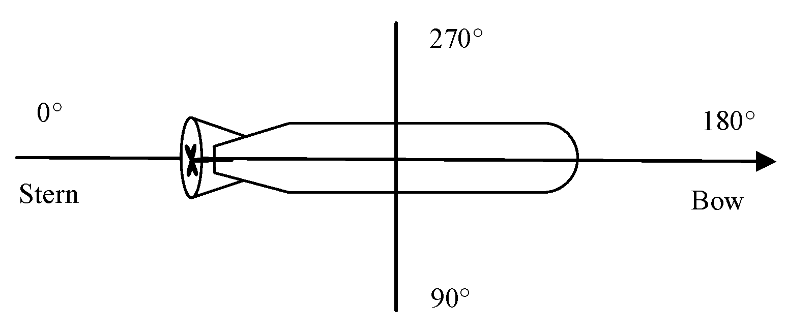
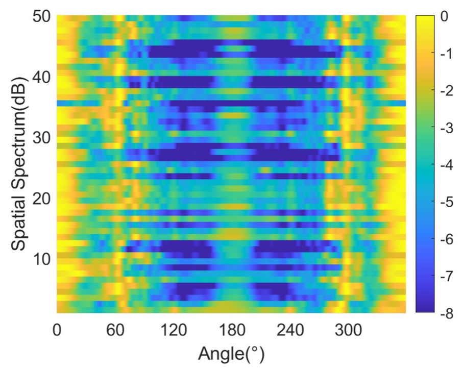
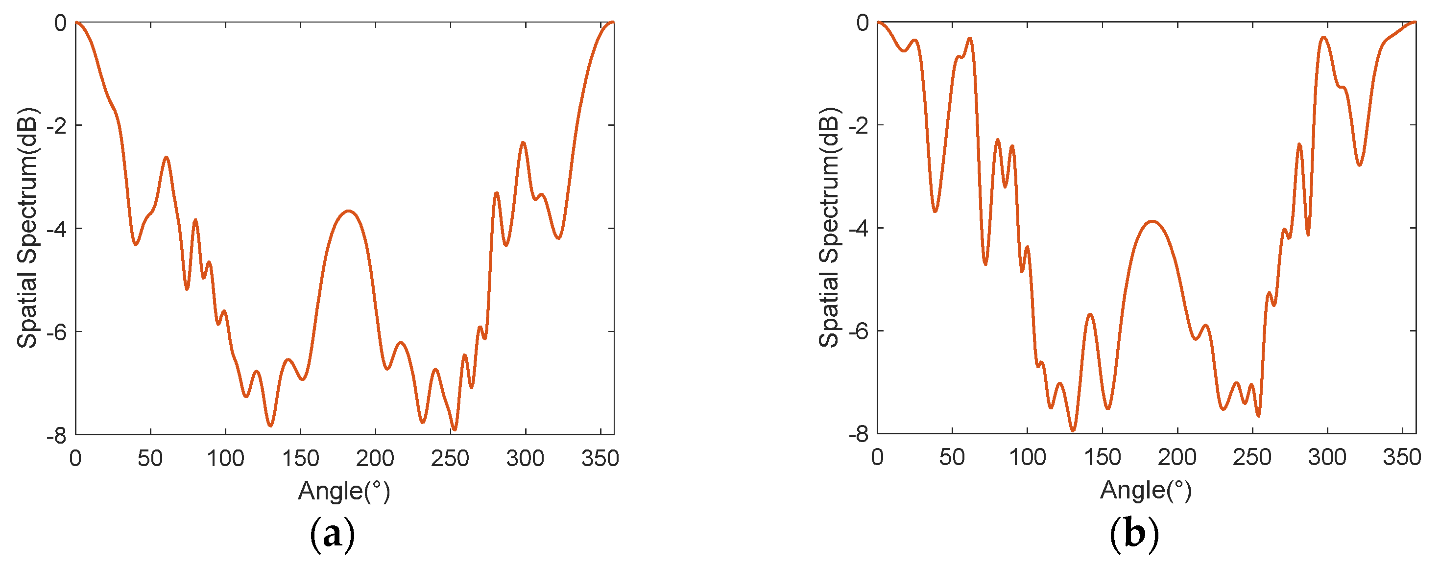
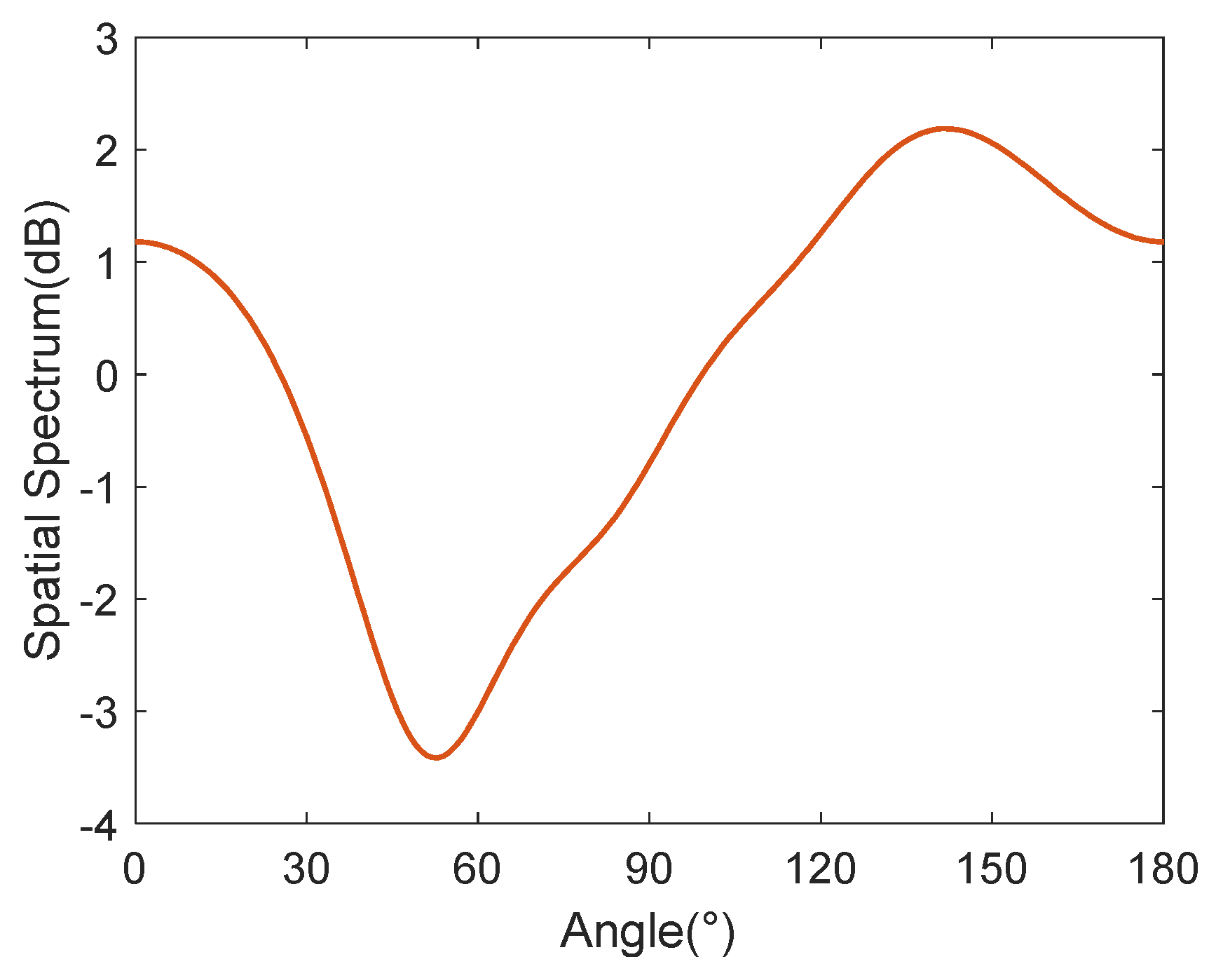
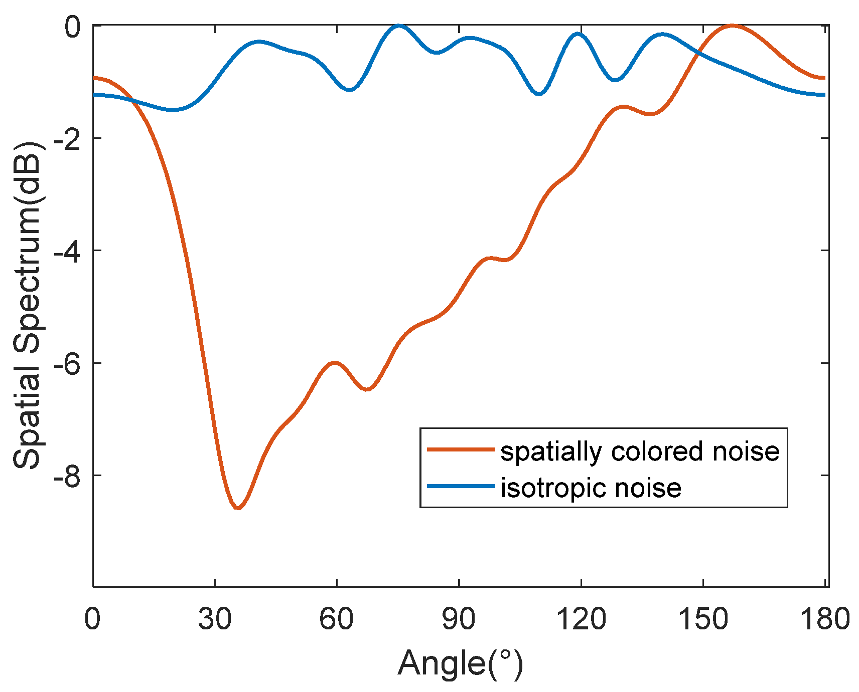
2.1. Spatial Distribution of Underwater Maneuvering Platform Noise

To explore the influence of the underwater maneuvering platform noise on DOA estimation using sonar arrays mounted on the platform, the noise spatial distribution was first analyzed. We processed 50 s data obtained from a sea trial. This segment of data were received by a 25-element linear array carried by an underwater maneuvering platform. It should be noted that during this period, there were no targets in the far-field. Therefore, it can be considered that the main part of the array receiving noise was the self-noise generated by the platform motion. The corresponding directions of the stern and bow of the underwater platform during the sea trial are shown in Figure 1.
As shown in Figure 1, 0° denotes the stern direction of the platform, and 180° denotes the bow direction. Figure 2 shows the bearing time record (BTR) of underwater platform noise in a certain frequency band using CBF. As shown, the underwater platform self-noise is obviously directional in the spatial domain. Due to the influence of the mechanical noise and the propeller noise, the spectrum level in the area near the stern of the platform (0–60°, 300–359°) is significantly higher than that in other areas. Additionally, the noise spectrum level in the area near the bow (170–190°) is also higher than that in the side area.
In order to show the spatial distribution of the noise more intuitively, Figure 3 shows the spatial spectrum at different times. Comparing Figure 3a,b, it is noticed that the noise spatial distribution varies from time to time, and it is hard to obtain a stationary noise covariance matrix [24]. Therefore, we need a DOA estimation method in an unknown SCN environment, which can provide a high estimation accuracy under limited array apertures and low SNR conditions.

2.2. Establishment of Noise Model

In this subsection, we divide the noise into two parts. One minor part is the isotropic noise, representing the environmental noise. The other major part is the SCN, representing the underwater maneuvering platform noise.
According to [25], we make the following assumptions for the isotropic noise:
(1)
Assume that there is a spherical surface on which Nw discrete points are randomly distributed.
(2)
Each discrete point is placed with independent narrow-band noise with the same power.
(3)
A receiving array is placed at the sphere center, and the sphere radius is significantly large compared to the array aperture. Therefore, the noise is approximated as a plane wave.
Following the above assumptions, the received isotropic noise data can be expressed as
n F F = i = 1 N w a F θ i , φ i s θ i , φ i
where θ i denotes the azimuth angle, φ i denotes the elevation angle, and s θ i , φ i denotes the received noise generated at θ i , φ i . Assume an M-element uniform linear array (ULA); a F θ i , φ i denotes the steering vector of the noise at θ i , φ i , shown as
a F ( θ i , φ i ) = 1 , exp ( j w d cos θ i cos φ i ) , , exp ( j w ( M 1 ) d cos θ i cos φ i ) T
where d is the element spacing, w = 2 π / λ is the wavenumber, and λ is the wavelength.
Similar to the isotropic noise condition, the SCN can be represented by adding enough discrete noise sources in some regions of the near field, denoted as
n N F = k = 1 N c a N r k s r k
where Nc is the number of near-field discrete noise sources. r k is the distance from the k-th near-field noise source to the reference element. a N r k is the near-field steering vector, denoted as
a N ( r k ) = 1 , r k r 2 k exp ( j w ( r 2 k r k ) ) , , r k r M k exp ( j w ( r M k r k ) ) T
where r M k denotes the distance from the k-th noise source to the M-th element.
Therefore, the underwater platform noise can be expressed as
n = n N F + n F F = k = 1 N c a N r k s r k + i = 1 N w a F θ i , φ i s θ i , φ i
To verify the effectiveness of the noise model, Figure 4 shows the spatial spectrum of the simulation noise. As shown, the noise is spatially colored, and the spectrum level is higher near the endfire directions, which shows similarity to the noise spatial distribution presented in Figure 4.

2.3. Received Data Model

Assume that K signals are incident from the far-field, the received data model at snapshot t can be expressed as
x ( t ) = A ( θ ) s ( t ) + n ( t ) , t { 1 , 2 , , T }
where T represents the total snapshot number, A ( θ ) = [ a ( θ 1 ) , , a ( θ K ) ] , and a ( θ k ) is denoted as 1 , , exp ( j w ( M 1 ) d cos ( θ k ) ) T .
For the multi-snapshot case of the SR model, Equation (6) is extended as
X = A ¯ S ¯ + N
where N = [ n ( 1 ) , , n ( T ) ] , X = [ x ( 1 ) , , x ( T ) ] , A ¯ = [ a ( θ 1 ) , , a ( θ L ) ] is an overcomplete dictionary formed by the steering vectors corresponding to θ = { θ 1 , , θ L } , where L satisfies L M > K , and S ¯ = [ s ¯ ( 1 ) , , s ¯ ( T ) ] is the zero-padding extension of S .

3. Proposed Method

Since SBL achieves a high accuracy under low SNRs and small snapshot numbers compared to CBF and MUSIC, in this section, we first extend the SBL framework to that under an unknown SCN covariance matrix. Then, to reconstruct this noise covariance matrix, we project the received data covariance matrix to the noise subspace through a maximum likelihood method, and the final estimation results are obtained through multiple iterations. Unlike SCN-MSBL and DN-SpSF, the proposed method does not set a parameterized model to obtain an approximate representation of the noise, but it rather directly acquires the SCN covariance matrix by projecting the received data covariance matrix to the noise subspace.

3.1. Sparse Bayesian Learning Framework under an Unknown SCN Covariance Matrix

Assume that the signals and the noise are uncorrelated, and the received data from different snapshots are independent of each other. The probability density of the SCN is expressed as
p ( N ; Σ n ) = t = 1 T C N ( n ( t ) ; 0 , Σ n )
where Σ n represents the noise covariance matrix. It is worth noting that if the noise is isotropic white Gaussian noise, Σ n = σ 2 I , where σ 2 denotes the noise power. Since N exhibits correlation in the spatial domain, Σ n cannot be represented by a diagonal matrix.
Depending on the received data model provided in Equation (7), the likelihood function of X is expressed as
p ( X | S ¯ ; Σ n ) = t = 1 T π Σ n 1 exp x ( t ) A ¯ s ¯ ( t ) H Σ n 1 x ( t ) A ¯ s ¯ ( t )
where | · | denotes the determinant operation.
Assuming that S ¯ is zero-mean complex Gaussian and distributed in the spatial domain, it can be expressed as
p ( S ¯ ; γ ) = t = 1 T l = 1 L 1 π γ l exp | s ¯ l ( t ) | 2 γ l
where Γ = diag ( γ ) , the hyperparameter γ = [ γ 1 , γ 2 γ L ] 0 , and each γ l represents the signal power corresponding to θ l . s ¯ l ( t ) denotes the l-th element in s ¯ ( t ) . Then, the evidence p ( X ; γ , Σ n ) is expressed as
p ( X ; γ , Σ n ) = t = 1 T π Σ x 1 exp x H ( t ) Σ x 1 x ( t )
where Σ x represents the covariance matrix of X, expressed as
Σ x = A ¯ Γ A ¯ H + Σ n
Following the Bayesian framework, the posterior probability of S ¯ with respect to X can be derived by using Equations (9)–(11), expressed as
p ( S ¯ | X ; γ , Σ n ) = C N ( S ¯ | μ , Σ s ) = t = 1 T π Σ s 1 exp s ¯ ( t ) μ t H Σ s 1 s ¯ ( t ) μ t
where μ = [ μ 1 , μ 2 , , μ T ] represents the expectation of S ¯ , and Σ s represents the variance of S ¯ . To obtain the expressions of Σ s and μ , we rewrite Equation (9) to change the expression to that in the original SBL [11,12], shown as
p ( X | S ¯ ; Σ n ) = t = 1 T π Σ n 1 exp x ( t ) A ¯ s ¯ ( t ) H Σ n 1 x ( t ) A ¯ s ¯ ( t ) = t = 1 T π Σ n 1 exp x ˜ ( t ) A ˜ s ¯ ( t ) 2 2
where x ˜ ( t ) = Σ n 1 2 x ( t ) and A ˜ = Σ n 1 2 A ¯ . Using the Woodbury identity, Σ s and μ can be expressed as
Σ s = ( A ˜ H A ˜ + Γ 1 ) 1 = ( A ¯ H Σ n 1 A ¯ + Γ 1 ) 1 = Γ Γ A ¯ H ( A ¯ Γ A ¯ H + Σ n ) 1 A ¯ Γ
μ = Σ s A ˜ H X ˜ = Σ s A ¯ H Σ n 1 X = Γ A ¯ H ( A ¯ Γ A ¯ H + Σ n ) 1 X
It is obvious that the calculation of Σ s and μ needs the defined hyperparameters γ and Σ n . According to Equation (10), the distribution of S ¯ depends on γ , which means the value of γ will affect the final result of the sparse reconstruction. To obtain a more reasonable γ , we first obtain the log function of Equation (11) and neglect the constant term, i.e.,
log ( p ( X ; γ , Σ n ) ) T log | Σ x | tr ( X H Σ x 1 X )
where tr ( · ) represents the trace operation. By maximizing the above equation, the estimates of γ and Σ n are obtained. Here, we adopt the expectation maximization method to resolve this problem since it is hard to take the partial derivatives of γ and Σ n directly. Therefore, γ is represented as
γ l = μ l μ l H T + Σ s l , l
where μ l is the l-th row of μ , and Σ s l , l is the l-th diagonal element of Σ s .
Due to the fact that it is hard to acquire an accurate distribution of the SCN covariance matrix Σ n , we are not able to utilize the above method for updating. Therefore, it is necessary to acquire a new method to estimate Σ n .

3.2. SCN Covariance Matrix Estimation

We maximize the log function of Equation (9) with respect to the potential targets S κ . For a fixed Σ n and A ¯ κ , S κ is expressed as
S κ = ( A ¯ κ H Σ n 1 A ¯ κ ) 1 A ¯ κ Σ n 1 X
where κ is the number of potential targets, and A ¯ κ consists of the steering vectors corresponding to the κ highest peaks from A ¯ . When the target number K is known, κ = K , and S κ = S = ( A H Σ n 1 A ) 1 A H Σ n 1 X .
Thus, the noise N can be expressed as
N = X A S κ = P A X
where P A = I A ¯ κ ( A ¯ κ H Σ n 1 A ¯ κ ) 1 A ¯ κ H Σ n 1 .
Furthermore, Σ n is approximately denoted as
Σ n = N N H T = P A R ^ P A H
where R ^ = X X H / N denotes the sample covariance matrix. Therefore, Σ n retains most of the SCN information, and the final results are obtained through multiple iterative steps.

3.3. Iterative Steps and Computational Complexity

Since this proposed method is adapted to underwater maneuvering platform noise, it is named underwater maneuvering platform noise sparse Bayesian learning (UNSBL).
The iterative steps are as Algorithm 1:
Algorithm 1: Underwater maneuvering platform noise sparse Bayesian learning (UNSBL)
Input: X , A ¯ ;
Initialization: hyperparameters γ and Σ n ; maximum number of iterations i max ; iteration termination parameter ε ;
While not converge do
(1) Calculate Σ s and μ using Equations (15) and (16);
(2) Update γ using Equation (18);
(3) Update Σ n using Equation (21);
(4) If γ n e w γ o l d 2 / γ n e w 2 < ε or i = i max , break;
(5) Else, go to step (1);
(6) End if
End while
Output: γ ;
In subsequent experiments, initialize γ and Σ n as identity matrices, i max = 2000 , and ε = 10 4 .
According to the above steps, it can be seen that in each iteration, the calculations of μ , Σ s , and γ are almost the same as those of classical SBL methods. For the update of Σ n , O κ M 2 complex multiplications are added. The computational complexity of the conventional SBL methods is O M 2 L + M L T . Because κ < M L , the computational complexity of UNSBL is approximately the same as that of the conventional SBL methods.

4. Simulation Analysis

Several simulation experiments were conducted to test the performance of UNSBL in this section. We compared the performance with that of several existing methods mentioned above, including CBF, MUSIC, SBL, DN-SpSF, and SCN-MSBL. The regularization parameter of DN-SpSF was selected as 8 in the following experiments. Due to the non-uniform distribution of the noise probability density, in the case of SCN, SNR can be defined as
SNR = 10 lg 2 π E s t s * t 0 2 π v n θ d θ
where v n θ represents the noise power at θ .

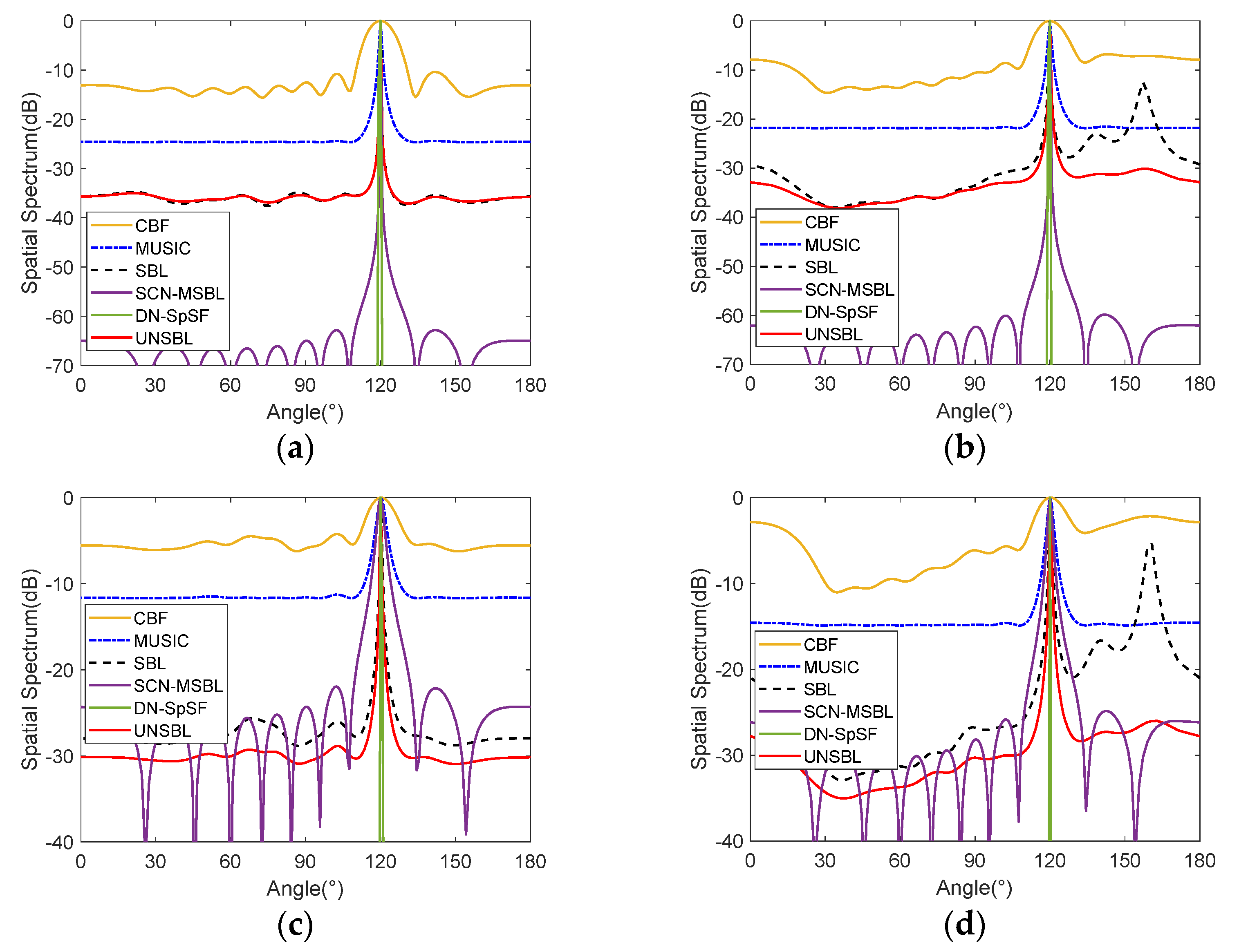
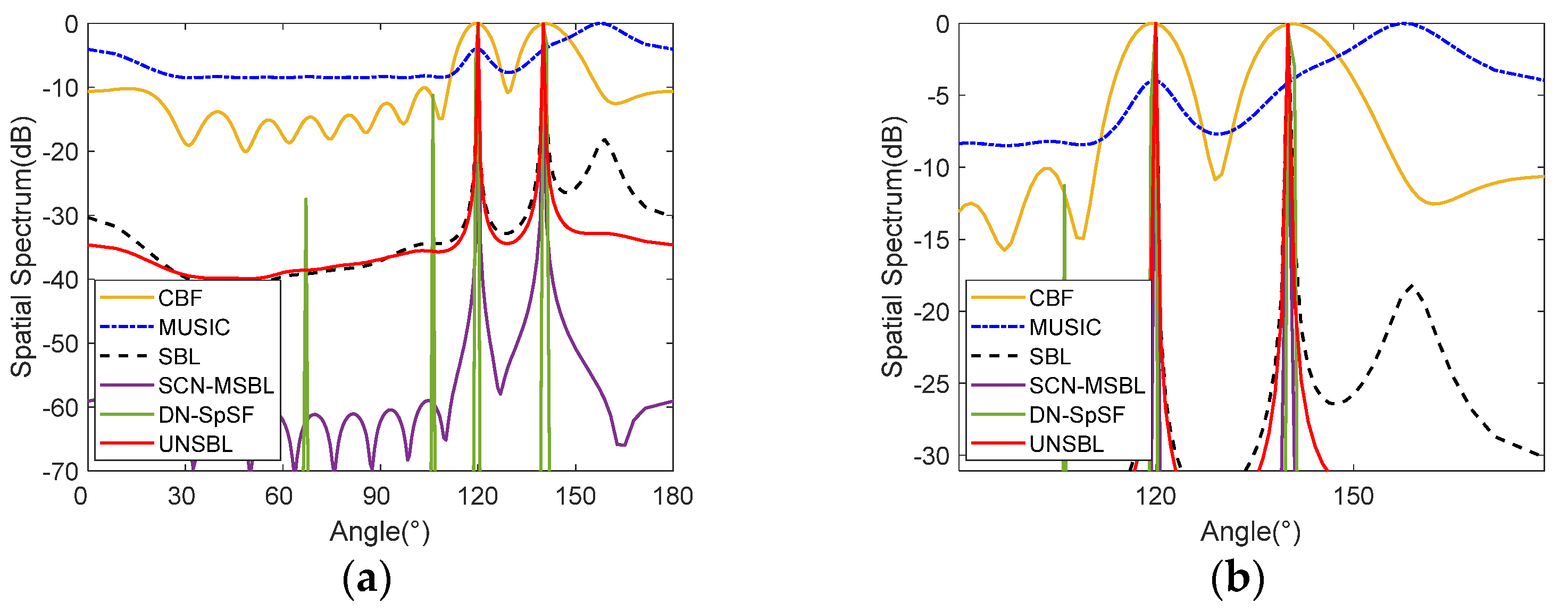
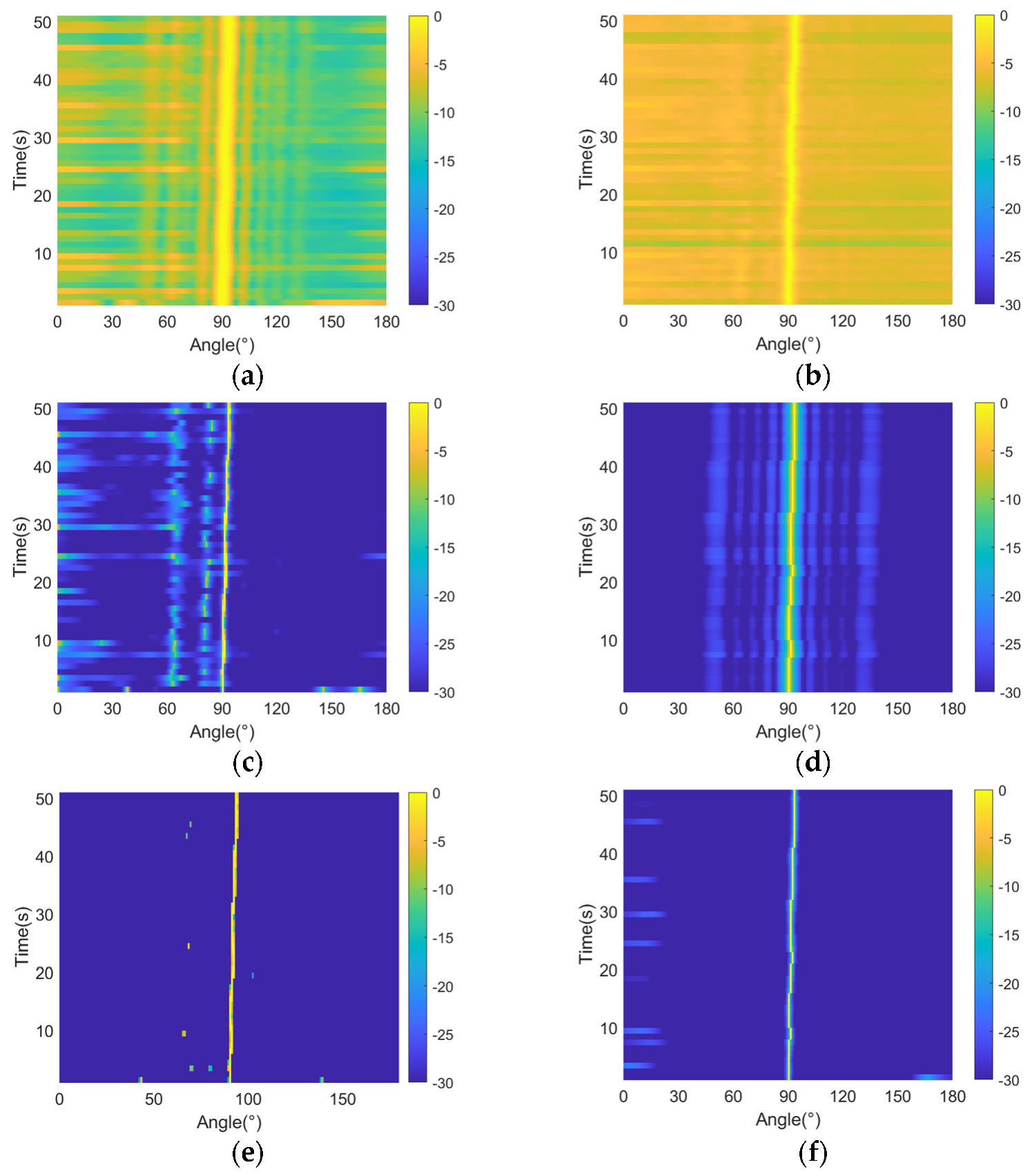
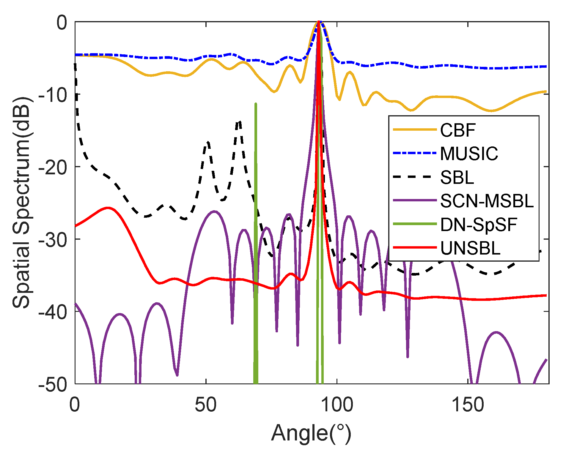
4.1. Spatial Spectra

First, the spatial spectrum estimation results of each method are examined in the presence of isotropic noise as well as SCN. Assume that a 10-element ULA with half-wavelength spacing is used to receive the source signal. A far-field narrowband signal is incident from 120°, the snapshot number is 100, and the discrete angle interval is set to 1°. The SCN model is established according to Section 2.2. Figure 5 shows the spatial spectra of the isotropic noise and the SCN received by the array in the case of no incident signal.
As shown, the spatial spectrum amplitude difference of the isotropic noise is within 2 dB. Unlike the isotropic noise, the simulated spatial spectrum amplitude difference of the SCN is about 9 dB. The peak and valley values of the noise appear around 160° and 30°, respectively. The noise spectrum level is higher near 0° and 180°, which is similar to the noise spatial distribution of the underwater platform mentioned in Section 2.2.
Next, we investigate the spatial spectra of the tested methods under different noise sources and SNRs. The results are shown in Figure 6.
As can be seen, the SR-based methods (SBL, SCN-MSBL, DN-SpSF, UNSBL) have sharper spectral peaks than MUSIC and CBF. Comparing Figure 6a,c and Figure 6b,d, we find that in the isotropic noise, all the tested methods can accurately estimate the target direction without spurious peaks. Moreover, the noise spectrum of each method is relatively flat, while under the SCN, the noise spectrum of CBF becomes higher in the ranges of 0–30° and 150–180°. The performance of SBL deteriorates under this situation. It has spurious peaks at 160° and 130°, which will cause misjudgment of the target in practical applications. MUSIC, SCN-MSBL, DN-SpSF, and the proposed UNSBL perform well under these two noise conditions. Thus, they are robust to different spatial distributions of noise. However, the performance of SCN-MSBL is greatly affected by SNRs.
Finally, we examine the spatial spectra of the tested methods with coherent signals. Assume that two coherent signals are incident from 120° and 140°, and the remaining simulation conditions are the same as in Figure 6d. Figure 7 shows the results of different methods.
As shown, MUSIC cannot deal with coherent signals, and the rest methods are able to estimate the DOAs. In Figure 7a, SBL still has spurious peaks due to the influence of SCN; it is worth noting that DN-SpSF generates spurious peaks because the regularization parameter used in the previous experiment is slightly small in this case. This fact indicates that the performance of DN-SpSF is sensitive to the selection of the regularization parameter. SCN-MSBL and the proposed UNSBL achieve good and robust performance with coherent signals compared to the other methods.

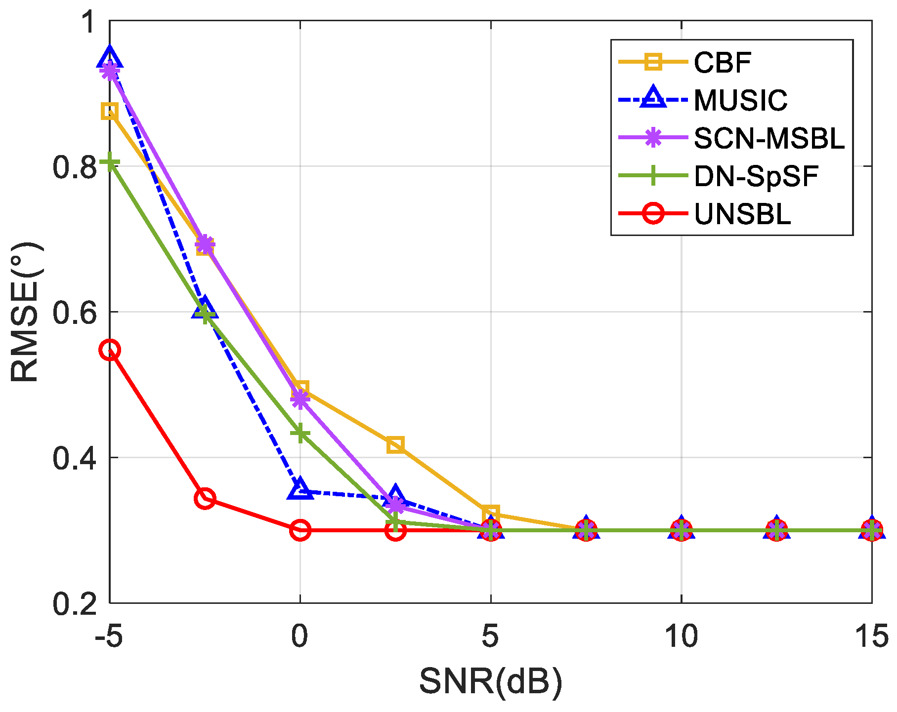
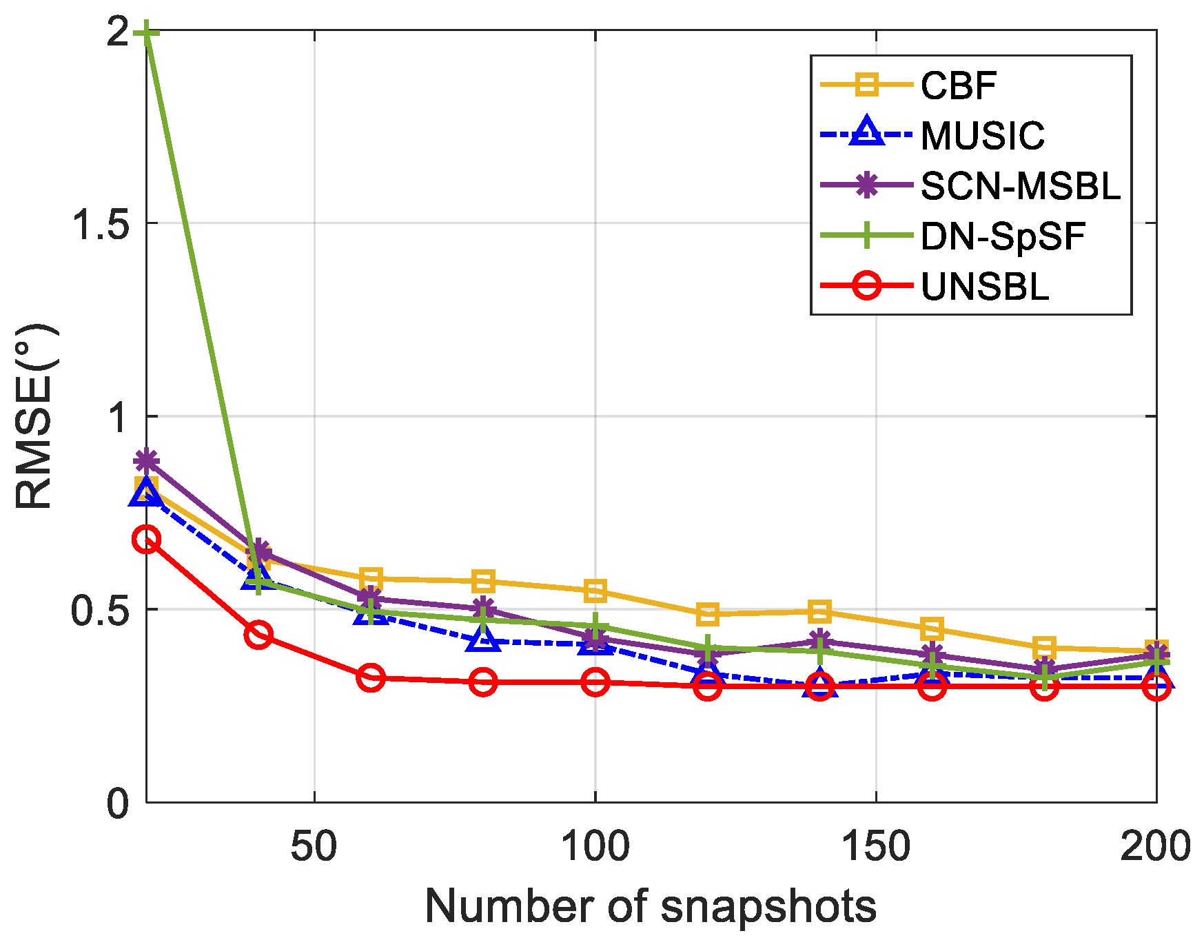
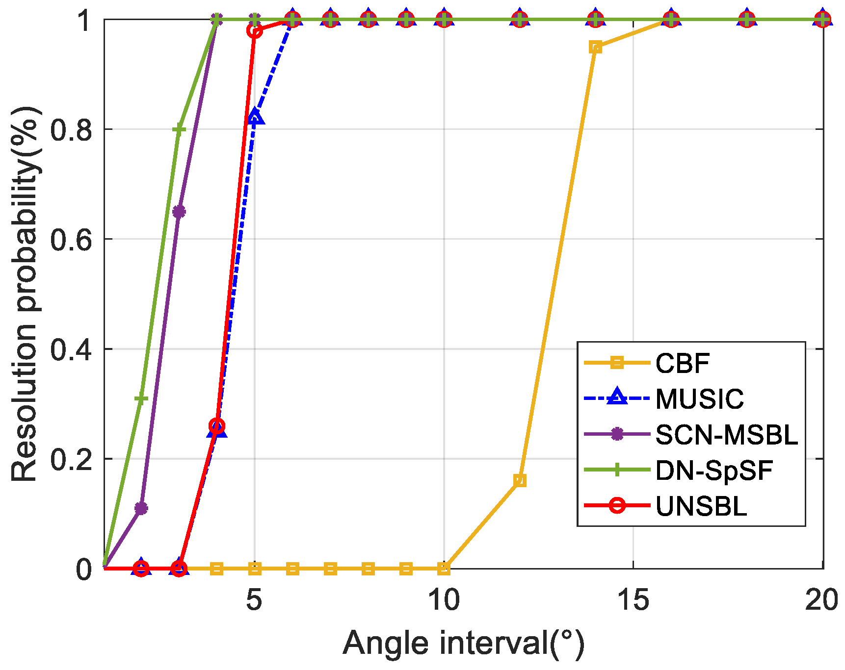
4.2. Statistical Performance
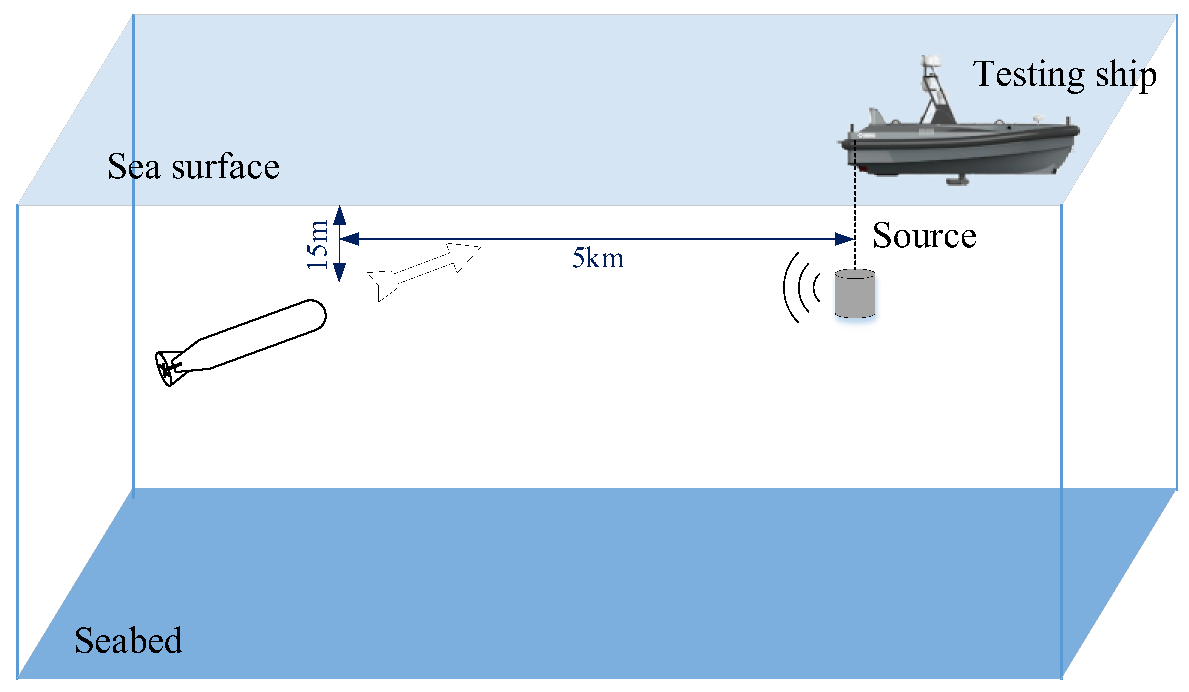
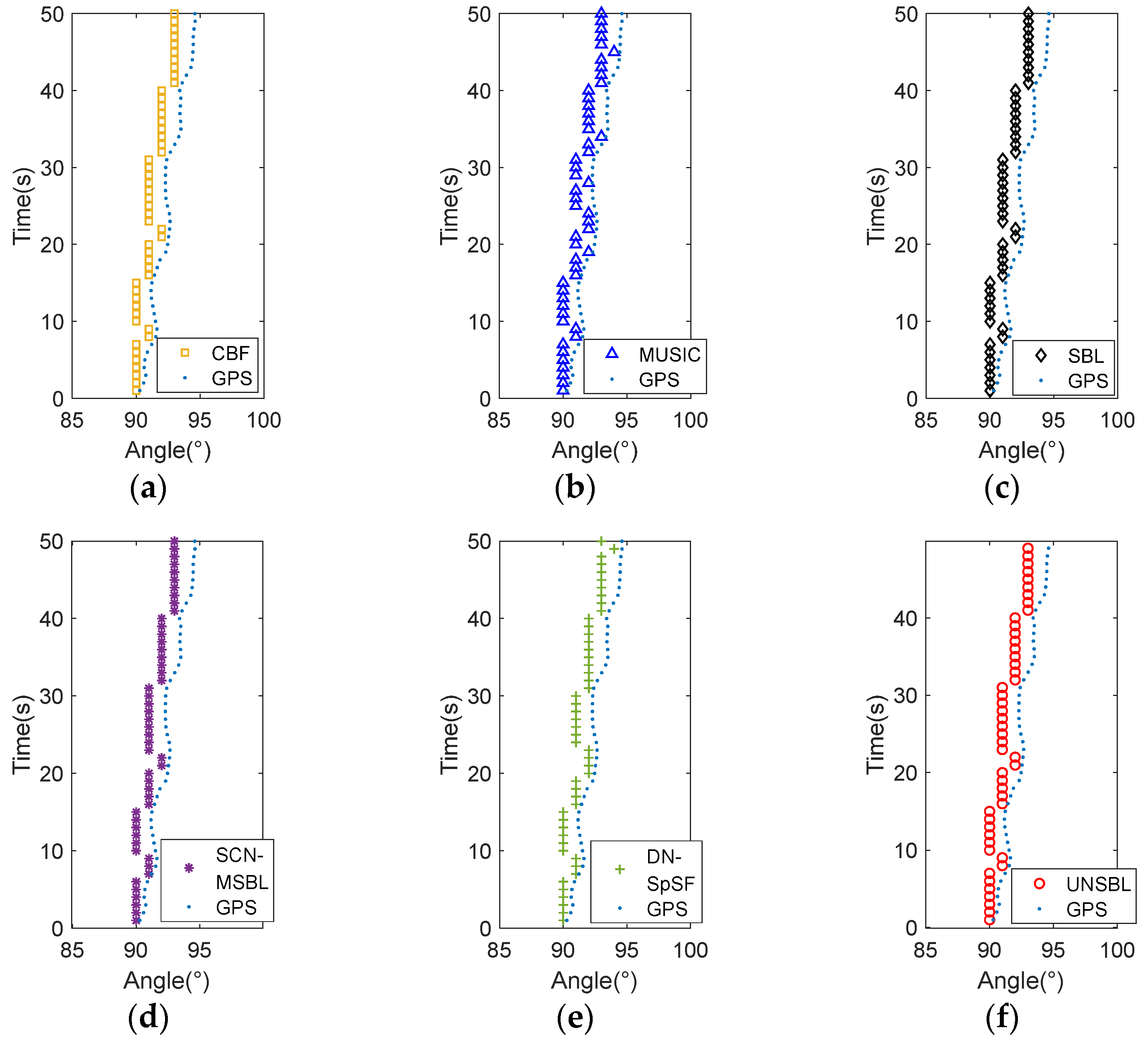
We analyze the statistical performance of the tested methods in SCN, including the root mean square errors (RMSEs) under different SNRs and different snapshot numbers, and the angle resolution ability of adjacent target signals. The SCN model is the same as that in Figure 5. The RMSE and the criteria for successfully distinguishing adjacent signals can be defined as follows
R M S E θ = 1 K × I i I k = 1 K θ ^ k i θ k 2
k = 1 2 θ ^ k i θ k < θ 1 θ 2
where I denotes the total number of Monte Carlo tests under each condition, and θ ^ k i is the i-th estimate of θ k .
First, assume that there are two uncorrelated far-field targets incident from 120.3° and 140.3°, respectively. The SNR changes from −5 dB to 15 dB, the discrete angle interval is 2°, the number of snapshots is 100, and 200 independent Monte Carlo tests are performed under each condition. Figure 8 shows the results of RMSE versus SNR. As shown, the proposed UNSBL provides a higher estimation accuracy, especially in the case of low SNRs. However, the other methods have higher RMSEs in such cases. Compared to them, the estimation accuracy of UNSBL is less affected when the SCN level becomes larger. Therefore, UNSBL is more robust than the other methods under low SNRs.
Then, the SNR is fixed at 0 dB, and the number of snapshots changes from 20 to 200. Figure 9 shows the results of RMSE versus the number of snapshots. As shown, DN-SpSF has the highest RMSE when the number of snapshots is 20. The overall RMSEs of CBF are slightly higher than those of the other methods. DN-SpSF provides the highest RMSEs when the number of snapshots is 20. UNSBL achieves a higher estimation accuracy than the other methods. In other words, the proposed UNSBL achieves better robustness under small snapshot numbers, compared to the rest methods.
Finally, assume that there are two adjacent signals incident from the far-field. We set the number of snapshots to 100 and SNR to 5 dB, and the angle interval between two adjacent signals increases from 4° to 20°. Figure 10 shows the resolution probability with different angle intervals. CBF performs the worst due to the Rayleigh limit. UNSBL is slightly better than MUSIC but inferior to SCN-MSBL and DN-SpSF. The reason is that Σ n is regarded as the projection of the received data covariance matrix in the noise space according to Equation (21). When the targets are spatially close, the similarity of the steering vectors of the two targets is too high, so the signal subspace bases are too similar, and they are easy to be judged as the same target.

5. Sea Trial

In this section, we test the effectiveness of UNSBL using the results of the sea trial data processing. The sea trial scenario is shown in Figure 11. The underwater mobile platform is equipped with a 25-elment linear array. The element spacing is half the wavelength corresponding to the highest frequency of the incident signal. In the sea trial, the underwater mobile platform sails at a depth of about 15 m. The source is suspended by the test ship in the water at a depth of about 15 m and placed at a distance of about 5 km from the underwater mobile platform.
We took 50 s received data and processed 200 frequency domain snapshots per second within a certain narrowband. The BTRs of CBF, MUSIC, SBL, SCN-MSBL, DN-SpSF, and the proposed UNSBL are shown in Figure 12. Here, 0° and 180° correspond to the stern and bow of the underwater platform, respectively. According to the GPS provided by the test ship, the target DOA changes from about 90° to about 94°. Figure 13 shows the GPS results and DOA results using different methods (ignoring the spurious peaks).
As shown in Figure 12 and Figure 13, all the tested methods can provide the approximate DOA estimation (all RMSEs are about 1.2°) while the performance varies considerably. In Figure 12a, CBF is affected by the local noise, and the noise spectrum level is generally high from 0° to 60°. In Figure 12b, the noise spectrum level of MUSIC is the highest. Comparing the BTRs of the SR-based methods shown in Figure 12c–f shows that SBL has multiple spurious peaks from 0° to 80° due to the local noise, which may be misjudged as spurious signals. DN-SpSF provides the lowest noise spectrum level while it has some spurious peaks at some time points. SCN-MSBL and the proposed UNSBL are highly suitable for the local noise, and UNSBL provides a lower noise spectrum level than SCN-MSBL. Then, we display the spatial spectra of the above methods at 45 s, and the results are shown in Figure 14. The difference between the highest and lowest noise spectrum levels is about 7 dB for CBF. DN-SpSF has the sharpest peak and the lowest noise spectrum level, while it has a spurious peak at about 60°. The proposed UNSBL has better performance with a lower and flatter noise spectrum level and a sharper peak compared to the rest methods.

6. Conclusions

For the sonar arrays fixed on an underwater maneuvering platform, the received noise is spatially directional, time-varying, and unknown. To estimate the DOAs of the far-field targets under such a condition and acquire better performance in low SNRs and small snapshot numbers, an SBL-based method is proposed in this paper, abbreviated as UNSBL. First, the SBL framework under an unknown noise covariance matrix is established. Then, this noise covariance matrix is estimated by projecting the covariance matrix of the received data into the noise subspace through a maximum likelihood method. The final DOA estimation results are obtained with multiple iterations. The proposed UNSBL performance and effectiveness are tested by simulation and sea trial data processing. The results show that UNSBL is superior in the following aspects:
(1)
UNSBL avoids spurious peaks and yields good and robust performance with various SNRs and coherent signals through spatial spectrum analysis.
(2)
UNSBL achieves a higher accuracy in the case of low SNRs and small snapshot numbers through statistical analysis, compared to the existing methods. In other words, UNSBL is more robust to such cases than the other methods.
(3)
The feasibility and stability of UNSBL are validated through sea trial data processing. UNSBL provides a lower and flatter noise spectrum level without spurious peaks in the real underwater maneuvering platform noise.
Although UNSBL has advantages in the above aspects, there are still some aspects that need to be improved. The major one is the resolution probability of UNSBL. We will continue to improve the capability of UNSBL in this aspect.

Author Contributions

Conceptualization, Y.W. and L.Z.; methodology, L.Z.; software, L.Z.; validation, L.Q. and J.W.; formal analysis, L.Z.; investigation, J.W.; resources, Y.W. and L.Q.; data curation, L.Z.; writing—original draft preparation, L.Z.; writing—review and editing, L.Q. and C.L.; visualization, L.Z.; supervision, Y.W.; project administration, Y.W.; funding acquisition, Y.W. All authors have read and agreed to the published version of the manuscript.

Funding

This research was funded by the National Natural Science Foundation of China (grant no. 62101153 and 62301183) and the Stable Supporting Fund of Acoustic Science and Technology Laboratory (grant no. JCKYS2021604SSJS003).

Institutional Review Board Statement

Not applicable.

Informed Consent Statement

Not applicable.

Data Availability Statement

Not applicable.

Conflicts of Interest

The authors declare no conflict of interest.

References

  1. Griffiths, L.; Jim, C. An Alternative Approach to Linearly Constrained Adaptive Beamforming. IEEE Trans. Antennas Propagat. 1982, 30, 27–34. [Google Scholar] [CrossRef]
  2. Capon, J. High-Resolution Frequency-Wavenumber Spectrum Analysis. Proc. IEEE 1969, 57, 1408–1418. [Google Scholar] [CrossRef]
  3. Hao, Y.; Zou, N.; Liang, G. Robust Capon Beamforming against Steering Vector Error Dominated by Large Direction-of-Arrival Mismatch for Passive Sonar. J. Mar. Sci. Eng. 2019, 7, 80. [Google Scholar] [CrossRef]
  4. Douglass, A.S.; Song, H.C.; Dowling, D.R. Performance Comparisons of Frequency-Difference and Conventional Beamforming. J. Acoust. Soc. Am. 2017, 142, 1663–1673. [Google Scholar] [CrossRef]
  5. Mañosas-Caballú, M.; Swindlehurst, A.L.; Seco-Granados, G. Power-Based Capon Beamforming: Avoiding the Cancellation Effects of GNSS Multipath. Signal Process. 2021, 180, 107891. [Google Scholar] [CrossRef]
  6. Wagner, M.; Park, Y.; Gerstoft, P. Gridless DOA Estimation and Root-MUSIC for Non-Uniform Linear Arrays. IEEE Trans. Signal Process. 2021, 69, 2144–2157. [Google Scholar] [CrossRef]
  7. Schmidt, R. Multiple Emitter Location and Signal Parameter Estimation. IEEE Trans. Antennas Propagat. 1986, 34, 276–280. [Google Scholar] [CrossRef]
  8. Liu, A.; Yang, D.; Shi, S.; Zhu, Z.; Li, Y. Augmented Subspace MUSIC Method for DOA Estimation Using Acoustic Vector Sensor Array. IET Radar Sonar Navig. 2019, 13, 969–975. [Google Scholar] [CrossRef]
  9. Stoica, P.; Sharman, K.C. Maximum Likelihood Methods for Direction-of-Arrival Estimation. IEEE Trans. Acoust. Speech Signal Process. 1990, 38, 1132–1143. [Google Scholar] [CrossRef]
  10. Tipping, M.E. Sparse Bayesian Learning and the Relevance Vector Machine. J. Mach. Learn. Res. 2001, 1, 211–244. [Google Scholar]
  11. Liu, Z.-M.; Huang, Z.-T.; Zhou, Y.-Y. An Efficient Maximum Likelihood Method for Direction-of-Arrival Estimation via Sparse Bayesian Learning. IEEE Trans. Wirel. Commun. 2012, 11, 1–11. [Google Scholar] [CrossRef]
  12. Wipf, D.P.; Rao, B.D. An Empirical Bayesian Strategy for Solving the Simultaneous Sparse Approximation Problem. IEEE Trans. Signal Process. 2007, 55, 3704–3716. [Google Scholar] [CrossRef]
  13. Gerstoft, P.; Mecklenbrauker, C.F.; Xenaki, A.; Nannuru, S. Multisnapshot Sparse Bayesian Learning for DOA. IEEE Signal Process. Lett. 2016, 23, 1469–1473. [Google Scholar] [CrossRef]
  14. Dai, J.; So, H.C. Real-Valued Sparse Bayesian Learning for DOA Estimation with Arbitrary Linear Arrays. IEEE Trans. Signal Process. 2021, 69, 4977–4990. [Google Scholar] [CrossRef]
  15. Al-Shoukairi, M.; Schniter, P.; Rao, B.D. A GAMP-Based Low Complexity Sparse Bayesian Learning Algorithm. IEEE Trans. Signal Process. 2018, 66, 294–308. [Google Scholar] [CrossRef]
  16. Shi, S.-G.; Li, Y.; Zhu, Z.; Shi, J. Real-Valued Robust DOA Estimation Method for Uniform Circular Acoustic Vector Sensor Arrays Based on Worst-Case Performance Optimization. Appl. Acoust. 2019, 148, 495–502. [Google Scholar] [CrossRef]
  17. Crespo Marques, E.; Maciel, N.; Naviner, L.; Cai, H.; Yang, J. A Review of Sparse Recovery Algorithms. IEEE Access 2019, 7, 1300–1322. [Google Scholar] [CrossRef]
  18. Friedlander, B.; Weiss, A.J. Direction Finding Using Noise Covariance Modeling. IEEE Trans. Signal Process. 1995, 43, 1557–1567. [Google Scholar] [CrossRef]
  19. Li, M.; Lu, Y. Maximum Likelihood DOA Estimation in Unknown Colored Noise Fields. IEEE Trans. Aerosp. Electron. Syst. 2008, 44, 1079–1090. [Google Scholar] [CrossRef]
  20. Agrawal, M.; Prasad, S. A Modified Likelihood Function Approach to DOA Estimation in the Presence of Unknown Spatially Correlated Gaussian Noise Using a Uniform Linear Array. IEEE Trans. Signal Process. 2000, 48, 2743–2749. [Google Scholar] [CrossRef]
  21. Yang, L.; Yang, Y.; Wang, Y. Sparse Spatial Spectral Estimation in Directional Noise Environment. J. Acoust. Soc. Am. 2016, 140, EL263–EL268. [Google Scholar] [CrossRef]
  22. Yang, J.; Yang, Y.; Lu, J.; Yang, L. Iterative Methods for DOA Estimation of Correlated Sources in Spatially Colored Noise Fields. Signal Process. 2021, 185, 108100. [Google Scholar] [CrossRef]
  23. Liang, G.; Shi, Z.; Qiu, L.; Sun, S.; Lan, T. Sparse Bayesian Learning Based Direction-of-Arrival Estimation under Spatially Colored Noise Using Acoustic Hydrophone Arrays. J. Mar. Sci. Eng. 2021, 9, 127. [Google Scholar] [CrossRef]
  24. Wu, Y.; Hou, C.; Liao, G.; Guo, Q. Direction-of-Arrival Estimation in the Presence of Unknown Nonuniform Noise Fields. IEEE J. Ocean. Eng. 2006, 31, 504–510. [Google Scholar] [CrossRef]
  25. Cron, B.F.; Sherman, C.H. Spatial-Correlation Functions for Various Noise Models. J. Acoust. Soc. Am. 1962, 34, 1732–1736. [Google Scholar] [CrossRef]
Figure 1. The corresponding directions of the stern and bow of the underwater platform.
Jmse 11 01879 g001
Figure 2. BTR of the underwater platform noise.
Jmse 11 01879 g002
Figure 3. The noise spatial spectrum at different times. (a) 17th s, (b) 32nd s.
Jmse 11 01879 g003
Figure 4. Spatial spectrum of the simulation noise.
Jmse 11 01879 g004
Figure 5. Spatial spectra of different noise sources.
Jmse 11 01879 g005
Figure 6. Spatial spectra under different noise sources and SNRs. (a) Isotropic noise SNR = 5 dB, (b) SCN SNR = 5 dB, (c) Isotropic noise SNR = −5 dB, (d) SCN SNR = −5 dB.
Jmse 11 01879 g006
Figure 7. Spatial spectra with coherent signals under SNR = 5 dB. (a) Spatial spectra, (b) Partial enlarged view.
Jmse 11 01879 g007
Figure 8. RMSE versus SNR.
Jmse 11 01879 g008
Figure 9. RMSE versus the number of snapshots.
Jmse 11 01879 g009
Figure 10. Resolution probability with different angle intervals.
Jmse 11 01879 g010
Figure 11. Sea trial situation.
Jmse 11 01879 g011
Figure 12. BTRs of different methods. (a) CBF, (b) MUSIC, (c) SBL, (d) SCN-MSBL, (e) DN-SpSF, and (f) UNSBL.
Jmse 11 01879 g012
Figure 13. GPS results and DOA results using different methods. (a) CBF, (b) MUSIC, (c) SBL, (d) SCN-MSBL, (e) DN-SpSF, and (f) UNSBL.
Jmse 11 01879 g013
Figure 14. Spatial spectra of different methods.
Jmse 11 01879 g014
Disclaimer/Publisher’s Note: The statements, opinions and data contained in all publications are solely those of the individual author(s) and contributor(s) and not of MDPI and/or the editor(s). MDPI and/or the editor(s) disclaim responsibility for any injury to people or property resulting from any ideas, methods, instructions or products referred to in the content.

