
Predicting Compound Coastal Flooding in Embayment-Backed Urban Catchments: Seawall and Storm Drain Implications

Abstract
:1. Introduction
2. Methods
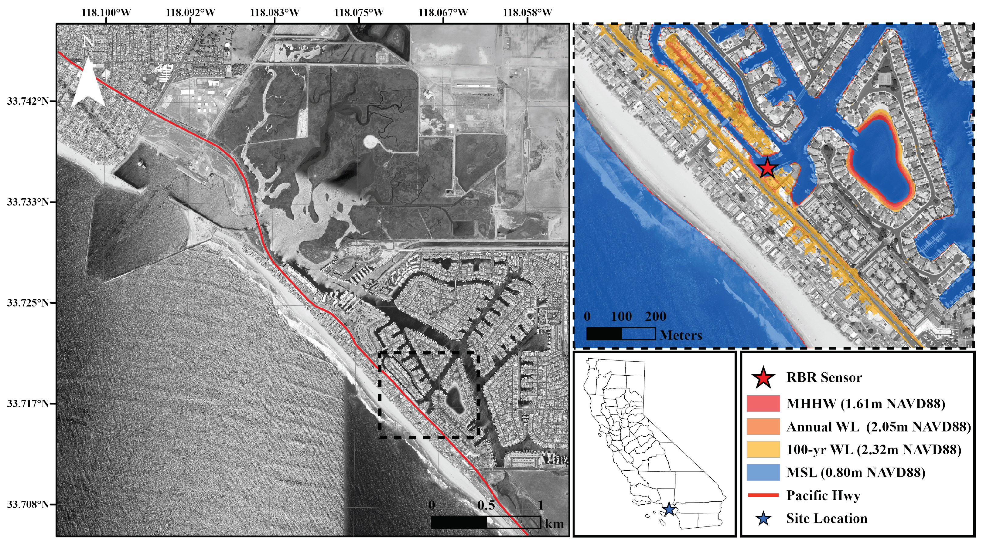
2.1. Site Description
2.2. Topographic and Bathymetric Data
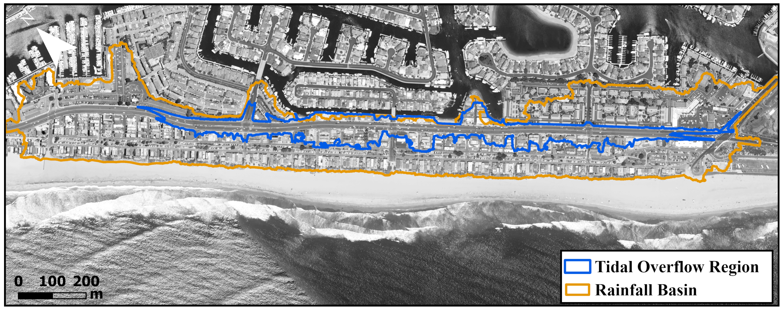
2.3. Identifying Compound Flooding Areas
2.4. Model
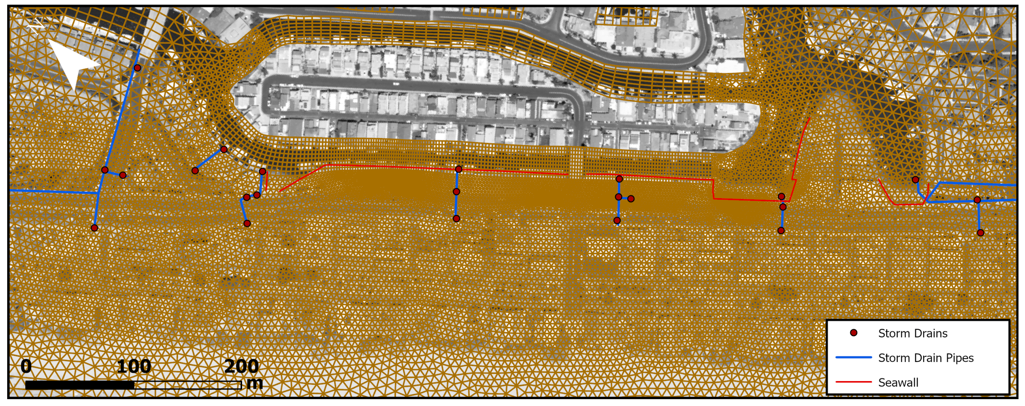
2.5. Model Setup
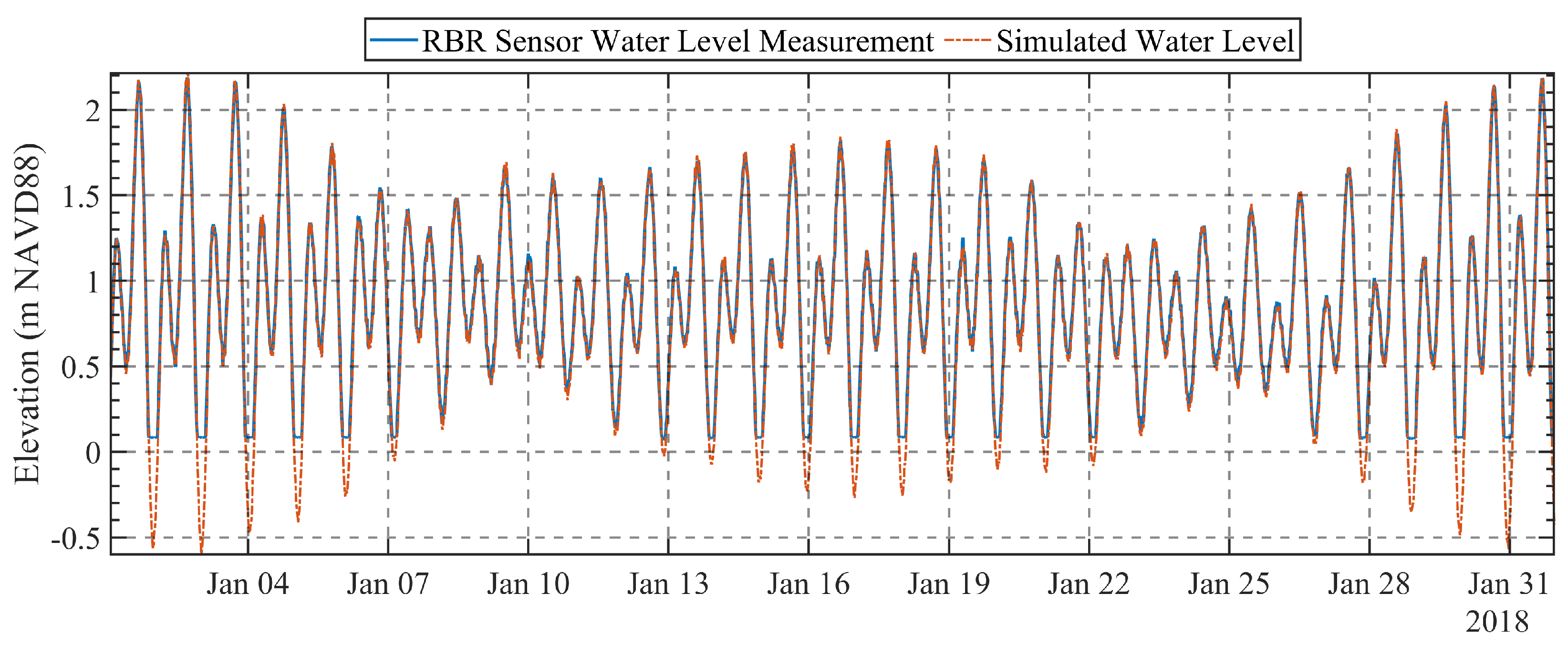
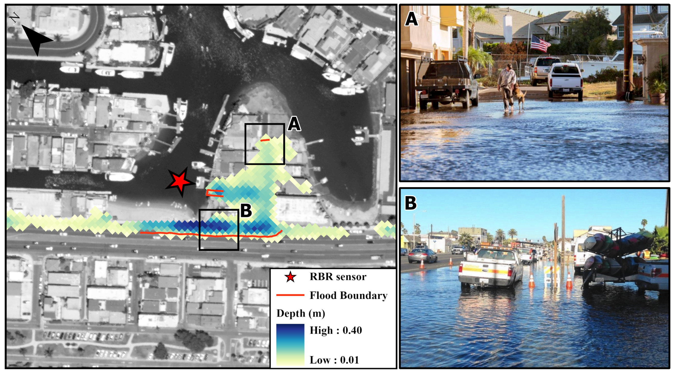
2.6. Model Validation
2.7. Extreme Event Analysis and Compound Event Design
2.8. Stormwater Drainage Models
3. Results
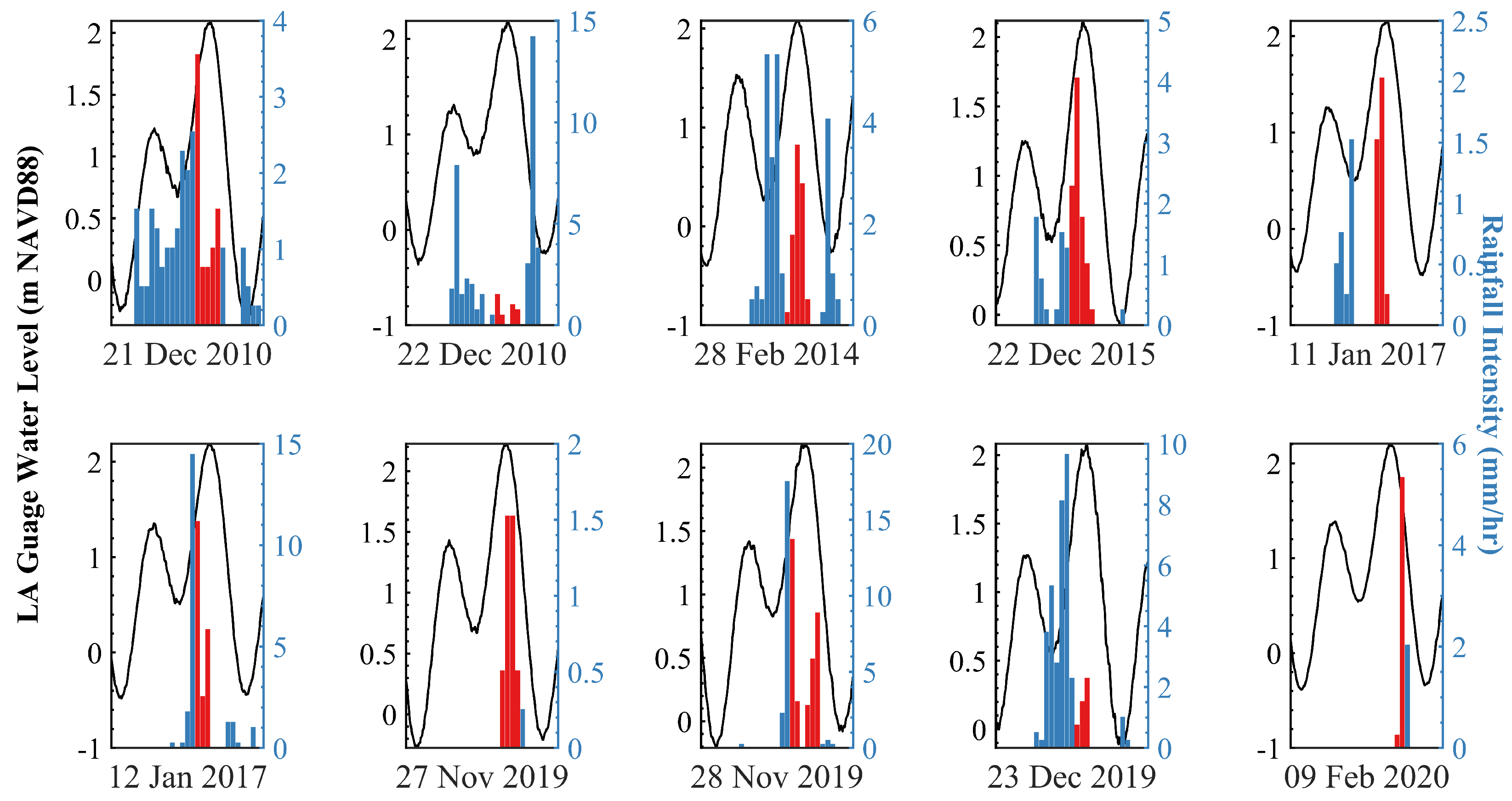
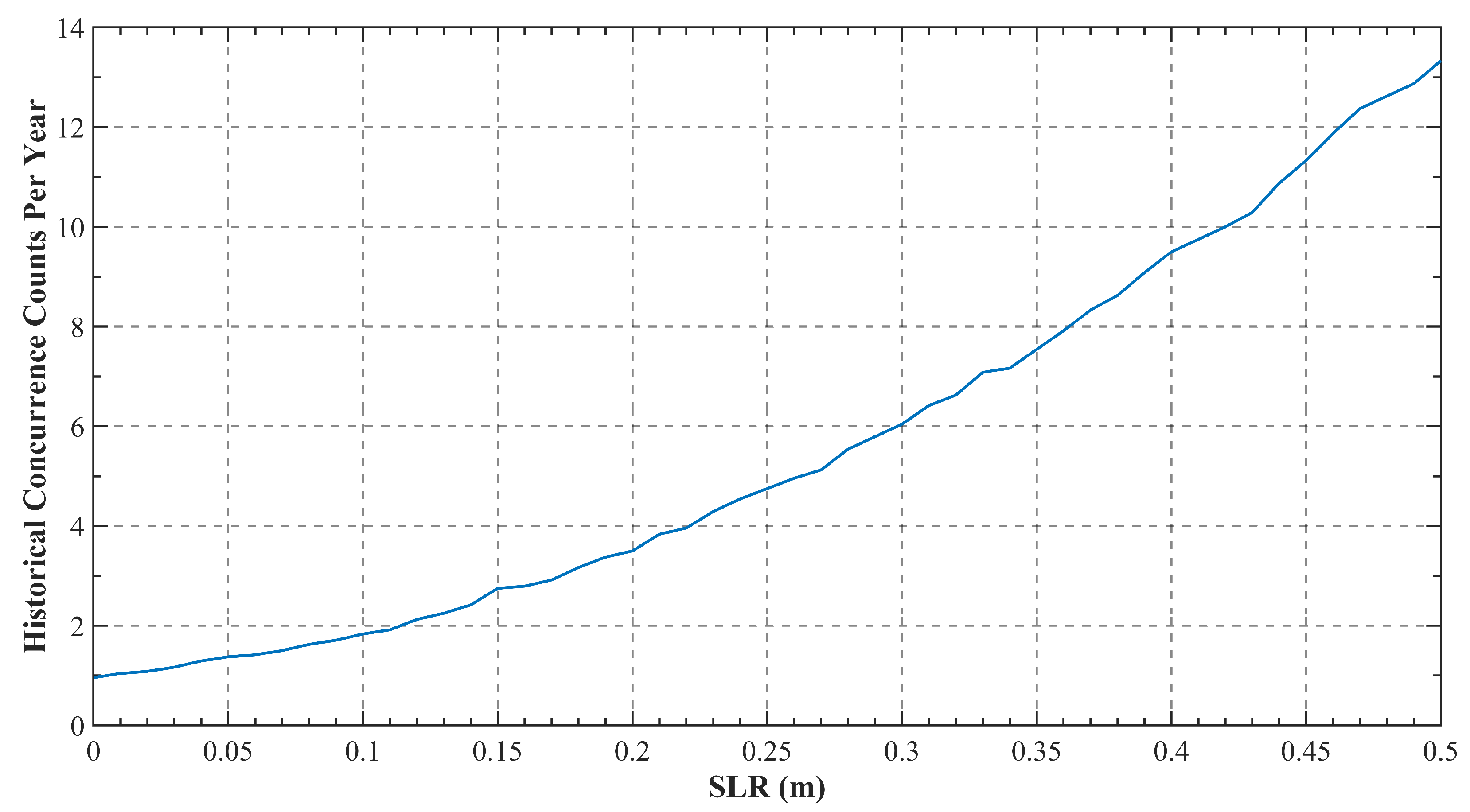
3.1. Historical Compound Flooding Analysis
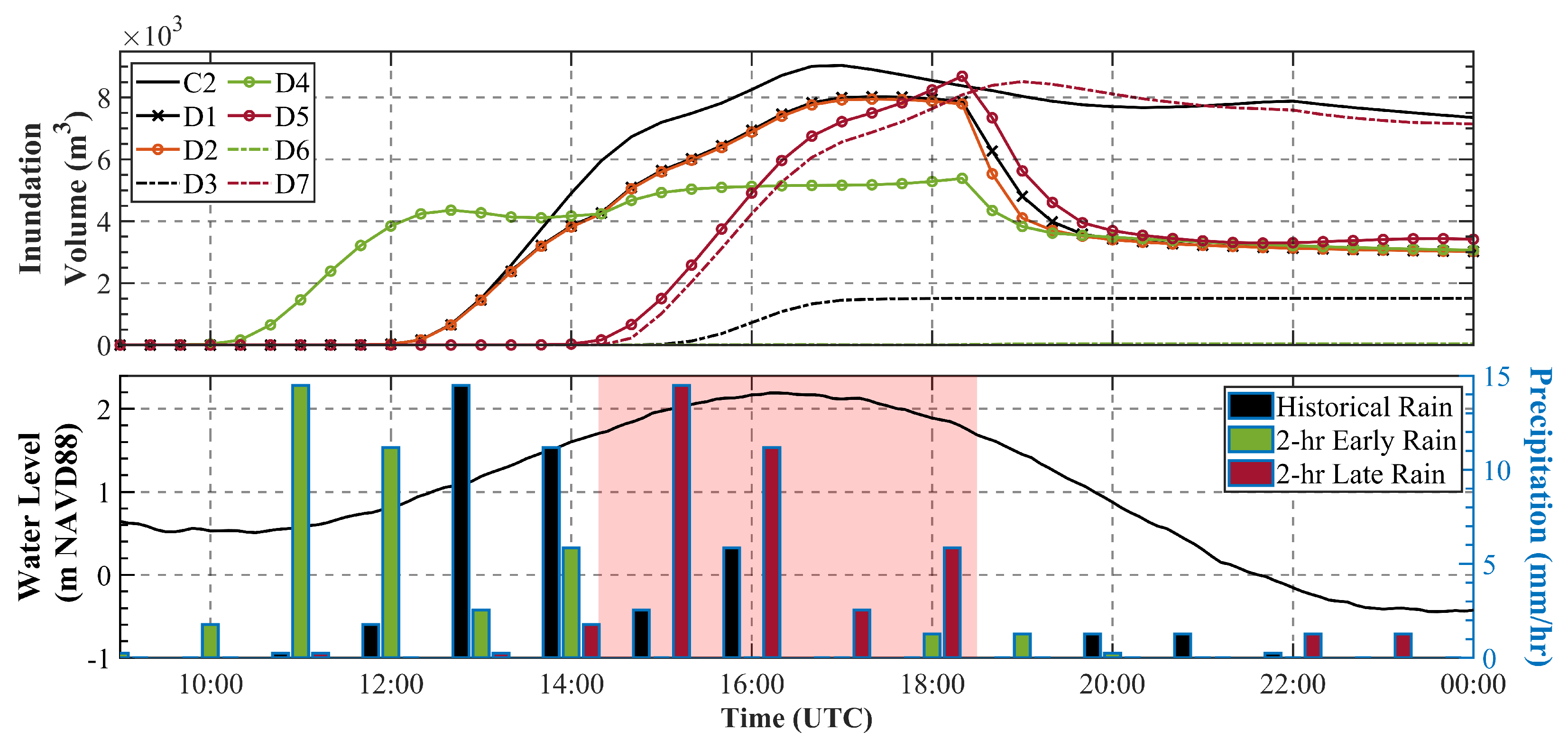
3.2. Subsurface Drainage System
4. Discussion
4.1. Precipitation and Tide Phasing
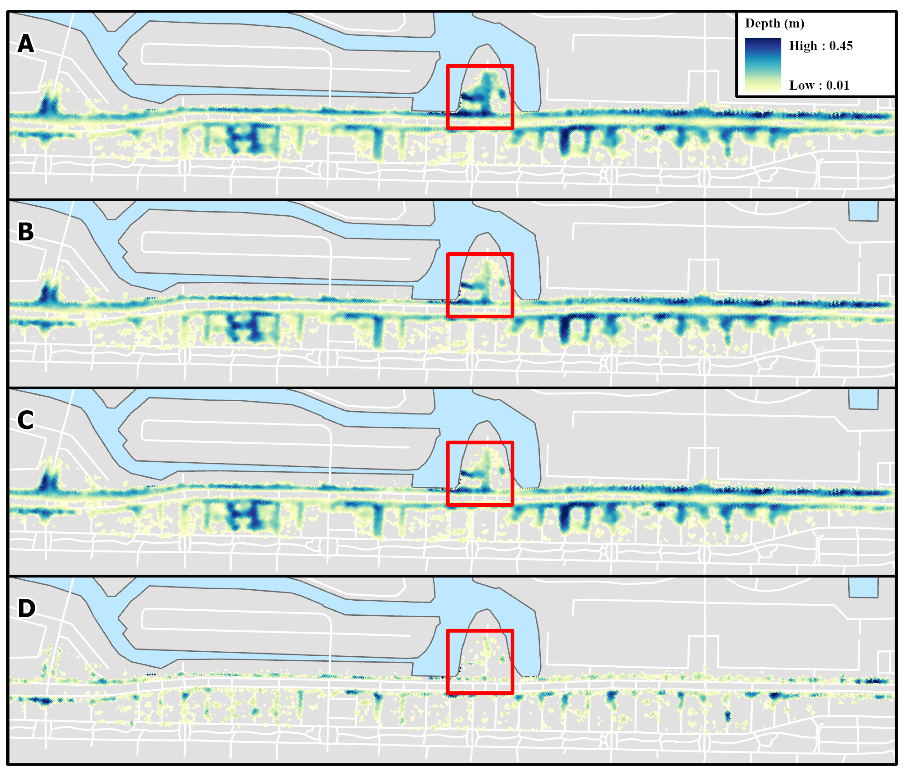
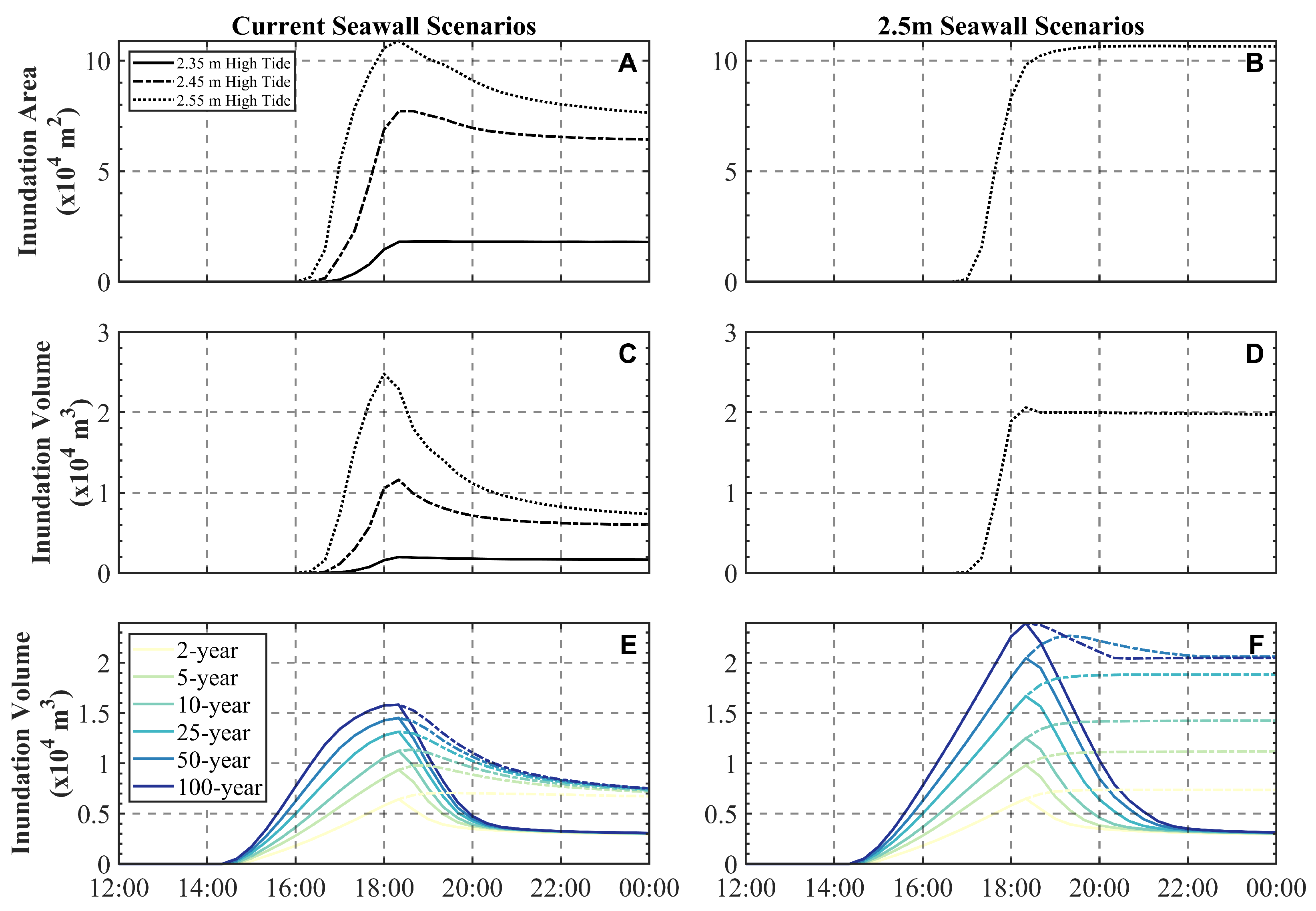
4.2. Seawall Impacts
5. Conclusions
Author Contributions
Funding
Institutional Review Board Statement
Informed Consent Statement
Data Availability Statement
Acknowledgments
Conflicts of Interest
Abbreviations
| BIC | Bayesian information criterion |
| CO | Constant outflow |
| DEM | Digital elevation model |
| IDF | Intensity-duration-frequency |
| IO | Iterative outflow |
| LiDAR | Light detection and ranging |
| NAVD88 | North American Vertical Datum of 1988 |
| NSE | Nash–Sutcliffe efficiency |
| NOAA | National Oceanic and Atmospheric Administration |
| PCH | Pacific Coast Highway |
| RMSE | Root mean square error |
| RR | Reduced rainfall |
| RTK | Real-time kinematic |
| USGS | United States Geological Survey |
References
- NASEM. Framing the Challenge of Urban Flooding in the United States; National Academies of Sciences, Engineering, and Medicine and Others; National Academies Press: Washington, DC, USA, 2019. [Google Scholar]
- Vitousek, S.; Barnard, P.L.; Fletcher, C.H.; Frazer, N.; Erikson, L.; Storlazzi, C.D. Doubling of coastal flooding frequency within decades due to sea-level rise. Sci. Rep. 2017, 7, 1399. [Google Scholar] [CrossRef] [PubMed] [Green Version]
- Taherkhani, M.; Vitousek, S.; Barnard, P.L.; Frazer, N.; Anderson, T.R.; Fletcher, C.H. Sea-level rise exponentially increases coastal flood frequency. Sci. Rep. 2020, 10, 6466. [Google Scholar] [CrossRef] [PubMed] [Green Version]
- Barnard, P.L.; van Ormondt, M.; Erikson, L.H.; Eshleman, J.; Hapke, C.; Ruggiero, P.; Adams, P.N.; Foxgrover, A.C. Development of the Coastal Storm Modeling System (CoSMoS) for predicting the impact of storms on high-energy, active-margin coasts. Nat. Hazards 2014, 74, 1095–1125. [Google Scholar] [CrossRef]
- Tebaldi, C.; Strauss, B.H.; Zervas, C.E. Modelling sea level rise impacts on storm surges along US coasts. Environ. Res. Lett. 2012, 7, 014032. [Google Scholar] [CrossRef]
- Moftakhari, H.R.; Salvadori, G.; AghaKouchak, A.; Sanders, B.F.; Matthew, R.A. Compounding effects of sea level rise and fluvial flooding. Proc. Natl. Acad. Sci. USA 2017, 114, 9785–9790. [Google Scholar] [CrossRef]
- Seneviratne, S.; Nicholls, N.; Easterling, D.; Goodess, C.; Kanae, S.; Kossin, J.; Luo, Y.; Marengo, J.; McInnes, K.; Rahimi, M.; et al. Changes in climate extremes and their impacts on the natural physical environment. In Managing the Risks of Extreme Events and Disasters to Advance Climate Change Adaptation; Cambridge University Press: Cambridge, UK, 2012. [Google Scholar]
- Field, C.B.; Barros, V.; Stocker, T.F.; Dahe, Q. Managing the Risks of Extreme Events and Disasters to Advance Climate Change Adaptation: Special Report of the Intergovernmental Panel on Climate Change; Cambridge University Press: Cambridge, UK, 2012. [Google Scholar]
- Zscheischler, J.; Westra, S.; Van Den Hurk, B.J.; Seneviratne, S.I.; Ward, P.J.; Pitman, A.; AghaKouchak, A.; Bresch, D.N.; Leonard, M.; Wahl, T.; et al. Future climate risk from compound events. Nat. Clim. Chang. 2018, 8, 469. [Google Scholar] [CrossRef]
- Ganguli, P.; Merz, B. Extreme coastal water levels exacerbate fluvial flood hazards in Northwestern Europe. Sci. Rep. 2019, 9, 13165. [Google Scholar] [CrossRef] [Green Version]
- Stephens, T.A.; Savant, G.; Sanborn, S.C.; Wallen, C.M.; Roy, S. Monolithic multiphysics simulation of compound flooding. J. Hydraul. Eng. 2022, 148, 05022003. [Google Scholar] [CrossRef]
- Wahl, T.; Jain, S.; Bender, J.; Meyers, S.D.; Luther, M.E. Increasing risk of compound flooding from storm surge and rainfall for major US cities. Nat. Clim. Chang. 2015, 5, 1093. [Google Scholar] [CrossRef]
- Bevacqua, E.; Maraun, D.; Vousdoukas, M.I.; Voukouvalas, E.; Vrac, M.; Mentaschi, L.; Widmann, M. Higher probability of compound flooding from precipitation and storm surge in Europe under anthropogenic climate change. Sci. Adv. 2019, 5, eaaw5531. [Google Scholar] [CrossRef] [Green Version]
- Gori, A.; Lin, N.; Smith, J. Assessing Compound Flooding from Landfalling Tropical Cyclones on the North Carolina Coast. Water Resour. Res. 2020, 56, e2019WR026788. [Google Scholar] [CrossRef] [Green Version]
- Song, H.; Kuang, C.; Gu, J.; Zou, Q.; Liang, H.; Sun, X.; Ma, Z. Nonlinear tide-surge-wave interaction at a shallow coast with large scale sequential harbor constructions. Estuar. Coast. Shelf Sci. 2020, 233, 106543. [Google Scholar] [CrossRef]
- Nederhoff, K.; Saleh, R.; Tehranirad, B.; Herdman, L.; Erikson, L.; Barnard, P.L.; Van der Wegen, M. Drivers of extreme water levels in a large, urban, high-energy coastal estuary—A case study of the San Francisco Bay. Coast. Eng. 2021, 170, 103984. [Google Scholar] [CrossRef]
- Herdman, L.; Erikson, L.; Barnard, P. Storm surge propagation and flooding in small tidal rivers during events of mixed coastal and fluvial influence. J. Mar. Sci. Eng. 2018, 6, 158. [Google Scholar] [CrossRef] [Green Version]
- Ward, P.J.; Couasnon, A.; Eilander, D.; Haigh, I.D.; Hendry, A.; Muis, S.; Veldkamp, T.I.; Winsemius, H.C.; Wahl, T. Dependence between high sea-level and high river discharge increases flood hazard in global deltas and estuaries. Environ. Res. Lett. 2018, 13, 084012. [Google Scholar] [CrossRef]
- Moftakhari, H.; Schubert, J.E.; AghaKouchak, A.; Matthew, R.A.; Sanders, B.F. Linking statistical and hydrodynamic modeling for compound flood hazard assessment in tidal channels and estuaries. Adv. Water Resour. 2019, 128, 28–38. [Google Scholar] [CrossRef]
- Couasnon, A.; Eilander, D.; Muis, S.; Veldkamp, T.I.; Haigh, I.D.; Wahl, T.; Winsemius, H.C.; Ward, P.J. Measuring compound flood potential from river discharge and storm surge extremes at the global scale. Nat. Hazards Earth Syst. Sci. 2020, 20, 489–504. [Google Scholar] [CrossRef] [Green Version]
- Muñoz, D.; Moftakhari, H.; Moradkhani, H. Compound Effects of Flood Drivers and Wetland Elevation Correction on Coastal Flood Hazard Assessment. Water Resour. Res. 2020, 56, e2020WR027544. [Google Scholar] [CrossRef]
- Santiago-Collazo, F.L.; Bilskie, M.V.; Hagen, S.C. A comprehensive review of compound inundation models in low-gradient coastal watersheds. Environ. Model. Softw. 2019, 119, 166–181. [Google Scholar] [CrossRef]
- Xu, K.; Wang, C.; Bin, L. Compound flood models in coastal areas: A review of methods and uncertainty analysis. Nat. Hazards 2022, 116, 469–496. [Google Scholar] [CrossRef]
- Hinkel, J.; Lincke, D.; Vafeidis, A.T.; Perrette, M.; Nicholls, R.J.; Tol, R.S.; Marzeion, B.; Fettweis, X.; Ionescu, C.; Levermann, A. Coastal flood damage and adaptation costs under 21st century sea-level rise. Proc. Natl. Acad. Sci. USA 2014, 111, 3292–3297. [Google Scholar] [CrossRef] [PubMed]
- Teng, J.; Vaze, J.; Dutta, D.; Marvanek, S. Rapid inundation modelling in large floodplains using LiDAR DEM. Water Resour. Manag. 2015, 29, 2619–2636. [Google Scholar] [CrossRef]
- Gallien, T.; Schubert, J.; Sanders, B. Predicting tidal flooding of urbanized embayments: A modeling framework and data requirements. Coast. Eng. 2011, 58, 567–577. [Google Scholar] [CrossRef]
- Gallien, T.; Sanders, B.; Flick, R. Urban coastal flood prediction: Integrating wave overtopping, flood defenses and drainage. Coast. Eng. 2014, 91, 18–28. [Google Scholar] [CrossRef]
- Ramirez, J.A.; Lichter, M.; Coulthard, T.J.; Skinner, C. Hyper-resolution mapping of regional storm surge and tide flooding: Comparison of static and dynamic models. Nat. Hazards 2016, 82, 571–590. [Google Scholar] [CrossRef]
- Teng, J.; Jakeman, A.J.; Vaze, J.; Croke, B.F.; Dutta, D.; Kim, S. Flood inundation modelling: A review of methods, recent advances and uncertainty analysis. Environ. Model. Softw. 2017, 90, 201–216. [Google Scholar] [CrossRef]
- Neal, J.; Villanueva, I.; Wright, N.; Willis, T.; Fewtrell, T.; Bates, P. How much physical complexity is needed to model flood inundation? Hydrol. Process. 2012, 26, 2264–2282. [Google Scholar] [CrossRef] [Green Version]
- Costabile, P.; Costanzo, C.; Macchione, F. Performances and limitations of the diffusive approximation of the 2-d shallow water equations for flood simulation in urban and rural areas. Appl. Numer. Math. 2017, 116, 141–156. [Google Scholar] [CrossRef]
- Gallien, T.W.; Kalligeris, N.; Delisle, M.P.C.; Tang, B.X.; Lucey, J.T.; Winters, M.A. Coastal flood modeling challenges in defended urban backshores. Geosciences 2018, 8, 450. [Google Scholar] [CrossRef] [Green Version]
- Sanders, B.F. Evaluation of on-line DEMs for flood inundation modeling. Adv. Water Resour. 2007, 30, 1831–1843. [Google Scholar] [CrossRef]
- Gallien, T. Validated coastal flood modeling at Imperial Beach, California: Comparing total water level, empirical and numerical overtopping methodologies. Coast. Eng. 2016, 111, 95–104. [Google Scholar] [CrossRef] [Green Version]
- Didier, D.; Bernatchez, P.; Boucher-Brossard, G.; Lambert, A.; Fraser, C.; Barnett, R.L.; Van-Wierts, S. Coastal flood assessment based on field debris measurements and wave runup empirical model. J. Mar. Sci. Eng. 2015, 3, 560–590. [Google Scholar] [CrossRef]
- Fewtrell, T.J.; Duncan, A.; Sampson, C.C.; Neal, J.C.; Bates, P.D. Benchmarking urban flood models of varying complexity and scale using high resolution terrestrial LiDAR data. Phys. Chem. Earth Parts A/B/C 2011, 36, 281–291. [Google Scholar] [CrossRef]
- Wang, Y.; Chen, A.S.; Fu, G.; Djordjević, S.; Zhang, C.; Savić, D.A. An integrated framework for high-resolution urban flood modelling considering multiple information sources and urban features. Environ. Model. Softw. 2018, 107, 85–95. [Google Scholar] [CrossRef]
- Bates, P.D.; Quinn, N.; Sampson, C.; Smith, A.; Wing, O.; Sosa, J.; Savage, J.; Olcese, G.; Neal, J.; Schumann, G.; et al. Combined modeling of US fluvial, pluvial, and coastal flood hazard under current and future climates. Water Resour. Res. 2021, 57, e2020WR028673. [Google Scholar] [CrossRef]
- Pelling, H.E.; Green, J.M. Impact of flood defences and sea-level rise on the European Shelf tidal regime. Cont. Shelf Res. 2014, 85, 96–105. [Google Scholar] [CrossRef]
- Lee, S.B.; Li, M.; Zhang, F. Impact of sea level rise on tidal range in Chesapeake and Delaware Bays. J. Geophys. Res. Oceans 2017, 122, 3917–3938. [Google Scholar] [CrossRef]
- Jia, G.; Wang, R.Q.; Stacey, M.T. Investigation of impact of shoreline alteration on coastal hydrodynamics using Dimension REduced Surrogate based Sensitivity Analysis. Adv. Water Resour. 2019, 126, 168–175. [Google Scholar] [CrossRef] [Green Version]
- Wadey, M.P.; Nicholls, R.J.; Hutton, C. Coastal flooding in the Solent: An integrated analysis of defences and inundation. Water 2012, 4, 430–459. [Google Scholar] [CrossRef] [Green Version]
- Huang, W.; Zhang, Y.J.; Liu, Z.; Yu, H.C.; Liu, Y.; Lamont, S.; Zhang, Y.; Hirpa, F.; Li, T.; Baker, B.; et al. Simulation of compound flooding in Japan using a nationwide model. Nat. Hazards 2023, 117, 2693–2713. [Google Scholar] [CrossRef]
- Leandro, J.; Schumann, A.; Pfister, A. A step towards considering the spatial heterogeneity of urban key features in urban hydrology flood modelling. J. Hydrol. 2016, 535, 356–365. [Google Scholar] [CrossRef]
- Shen, Y.; Morsy, M.M.; Huxley, C.; Tahvildari, N.; Goodall, J.L. Flood risk assessment and increased resilience for coastal urban watersheds under the combined impact of storm tide and heavy rainfall. J. Hydrol. 2019, 579, 124159. [Google Scholar] [CrossRef]
- Shi, S.; Yang, B.; Jiang, W. Numerical simulations of compound flooding caused by storm surge and heavy rain with the presence of urban drainage system, coastal dam and tide gates: A case study of Xiangshan, China. Coast. Eng. 2022, 172, 104064. [Google Scholar] [CrossRef]
- Zhang, S.; Pan, B. An urban storm-inundation simulation method based on GIS. J. Hydrol. 2014, 517, 260–268. [Google Scholar] [CrossRef]
- Liu, L.; Liu, Y.; Wang, X.; Yu, D.; Liu, K.; Huang, H.; Hu, G. Developing an effective 2-D urban flood inundation model for city emergency management based on cellular automata. Nat. Hazards Earth Syst. Sci. 2015, 15, 381–391. [Google Scholar] [CrossRef] [Green Version]
- Smith, R.A.; Bates, P.D.; Hayes, C. Evaluation of a coastal flood inundation model using hard and soft data. Environ. Model. Softw. 2012, 30, 35–46. [Google Scholar] [CrossRef]
- NOAA. Extreme Water Levels 9410660 Los Angeles, CA, 2023. National Oceanic and Atmospheric Administration Website. 2023. Available online: https://tidesandcurrents.noaa.gov/est/est_station.shtml?stnid=9410660 (accessed on 22 May 2023).
- NOAA. 2009–2011 Merged Topobathy DEM, 2023. 2009–2011 CA Coastal Conservancy Coastal Lidar Project: Hydro-Flattened Bare Earth DEM from 2010 to 06-15 to 2010-08-15. Available online: https://www.fisheries.noaa.gov/inport/item/55761 (accessed on 22 May 2023).
- NOAA. 2014 USACE NCMP Topobathy Lidar DEM: California, 2023. Collected by the Joint Airborne Lidar Bathymetry Technical Center of Expertise (JALBTCX), Depicting the Elevations above and below the Immediate Coastal Waters. Available online: https://www.fisheries.noaa.gov/inport/item/49416 (accessed on 22 May 2023).
- Martyr-Koller, R.; Kernkamp, H.; van Dam, A.; van der Wegen, M.; Lucas, L.; Knowles, N.; Jaffe, B.; Fregoso, T. Application of an unstructured 3D finite volume numerical model to flows and salinity dynamics in the San Francisco Bay-Delta. Estuar. Coast. Shelf Sci. 2017, 192, 86–107. [Google Scholar] [CrossRef]
- Kumbier, K.; Cabral Carvalho, R.; Vafeidis, A.T.; Woodroffe, C.D. Investigating compound flooding in an estuary using hydrodynamic modelling: A case study from the Shoalhaven River, Australia. Nat. Hazards Earth Syst. Sci. 2018, 18, 463–477. [Google Scholar] [CrossRef] [Green Version]
- Lyddon, C.E.; Brown, J.M.; Leonardi, N.; Plater, A.J. Increased coastal wave hazard generated by differential wind and wave direction in hyper-tidal estuaries. Estuar. Coast. Shelf Sci. 2019, 220, 131–141. [Google Scholar] [CrossRef]
- Lyddon, C.E.; Brown, J.M.; Leonardi, N.; Saulter, A.; Plater, A.J. Quantification of the uncertainty in coastal storm hazard predictions due to wave-current interaction and wind forcing. Geophys. Res. Lett. 2019, 46, 14576–14585. [Google Scholar] [CrossRef] [Green Version]
- Serafin, K.A.; Ruggiero, P.; Parker, K.; Hill, D.F. What’s streamflow got to do with it? A probabilistic simulation of the competing oceanographic and fluvial processes driving extreme along-river water levels. Nat. Hazards Earth Syst. Sci. 2019, 19, 1415–1431. [Google Scholar] [CrossRef] [Green Version]
- Kvočka, D.; Falconer, R.A.; Bray, M. Appropriate model use for predicting elevations and inundation extent for extreme flood events. Nat. Hazards 2015, 79, 1791–1808. [Google Scholar] [CrossRef] [Green Version]
- Costabile, P.; Costanzo, C.; De Lorenzo, G.; Macchione, F. Is local flood hazard assessment in urban areas significantly influenced by the physical complexity of the hydrodynamic inundation model? J. Hydrol. 2020, 580, 124231. [Google Scholar] [CrossRef]
- Wang, J.; Gao, W.; Xu, S.; Yu, L. Evaluation of the combined risk of sea level rise, land subsidence, and storm surges on the coastal areas of Shanghai, China. Clim. Chang. 2012, 115, 537–558. [Google Scholar] [CrossRef]
- Uddin, M.; Alam, J.B.; Khan, Z.H.; Hasan, G.J.; Rahman, T. Two dimensional hydrodynamic modelling of Northern Bay of Bengal coastal waters. Comput. Water Energy Environ. Eng. 2014, 2014, 49792. [Google Scholar] [CrossRef] [Green Version]
- Thanh, V.Q.; Reyns, J.; Wackerman, C.; Eidam, E.F.; Roelvink, D. Modelling suspended sediment dynamics on the subaqueous delta of the Mekong River. Cont. Shelf Res. 2017, 147, 213–230. [Google Scholar] [CrossRef]
- Green, R.H.; Lowe, R.J.; Buckley, M.L. Hydrodynamics of a tidally forced coral reef atoll. J. Geophys. Res. Oceans 2018, 123, 7084–7101. [Google Scholar] [CrossRef]
- Symonds, A.M.; Vijverberg, T.; Post, S.; van der Spek, B.J.; Henrotte, J.; Sokolewicz, M. Comparison between mike 21 FM, delft3d and delft3d FM flow models of western port bay, Australia. Coast. Eng. 2016, 2, 1–12. [Google Scholar] [CrossRef] [Green Version]
- Kramer, S.C.; Stelling, G.S. A conservative unstructured scheme for rapidly varied flows. Int. J. Numer. Methods Fluids 2008, 58, 183–212. [Google Scholar] [CrossRef]
- Akoh, R.; Ishikawa, T.; Kojima, T.; Tomaru, M.; Maeno, S. High-resolution modeling of tsunami run-up flooding: A case study of flooding in Kamaishi city, Japan, induced by the 2011 Tohoku tsunami. Nat. Hazards Earth Syst. Sci. 2017, 17, 1871–1883. [Google Scholar] [CrossRef] [Green Version]
- Xie, D.; Zou, Q.P.; Mignone, A.; MacRae, J.D. Coastal flooding from wave overtopping and sea level rise adaptation in the northeastern USA. Coast. Eng. 2019, 150, 39–58. [Google Scholar] [CrossRef]
- Rong, Y.; Zhang, T.; Zheng, Y.; Hu, C.; Peng, L.; Feng, P. Three-dimensional urban flood inundation simulation based on digital aerial photogrammetry. J. Hydrol. 2020, 584, 124308. [Google Scholar] [CrossRef]
- Liu, Q.; Xu, H.; Wang, J. Assessing tropical cyclone compound flood risk using hydrodynamic modelling: A case study in Haikou City, China. Nat. Hazards Earth Syst. Sci. 2022, 22, 665–675. [Google Scholar] [CrossRef]
- Leroy, S.; Pedreros, R.; André, C.; Paris, F.; Lecacheux, S.; Marche, F.; Vinchon, C. Coastal flooding of urban areas by overtopping: Dynamic modelling application to the Johanna storm (2008) in Gâvres (France). Nat. Hazards Earth Syst. Sci. 2015, 15, 2497–2510. [Google Scholar] [CrossRef] [Green Version]
- Kernkamp, H.W.; Van Dam, A.; Stelling, G.S.; de Goede, E.D. Efficient scheme for the shallow water equations on unstructured grids with application to the Continental Shelf. Ocean Dyn. 2011, 61, 1175–1188. [Google Scholar] [CrossRef] [Green Version]
- Gallegos, H.A.; Schubert, J.E.; Sanders, B.F. Two-dimensional, high-resolution modeling of urban dam-break flooding: A case study of Baldwin Hills, California. Adv. Water Resour. 2009, 32, 1323–1335. [Google Scholar] [CrossRef]
- Bricker, J.D.; Gibson, S.; Takagi, H.; Imamura, F. On the need for larger Manning’s roughness coefficients in depth-integrated tsunami inundation models. Coast. Eng. J. 2015, 57, 1550005. [Google Scholar] [CrossRef]
- Schubert, J.E.; Sanders, B.F.; Smith, M.J.; Wright, N.G. Unstructured mesh generation and landcover-based resistance for hydrodynamic modeling of urban flooding. Adv. Water Resour. 2008, 31, 1603–1621. [Google Scholar] [CrossRef]
- Brown, J.D.; Spencer, T.; Moeller, I. Modeling storm surge flooding of an urban area with particular reference to modeling uncertainties: A case study of Canvey Island, United Kingdom. Water Resour. Res. 2007, 43. [Google Scholar] [CrossRef] [Green Version]
- Lyddon, C.; Brown, J.M.; Leonardi, N.; Plater, A.J. Flood hazard assessment for a hyper-tidal estuary as a function of tide-surge-morphology interaction. Estuaries Coasts 2018, 41, 1565–1586. [Google Scholar] [CrossRef] [Green Version]
- Lyddon, C.; Brown, J.M.; Leonardi, N.; Plater, A.J. Uncertainty in estuarine extreme water level predictions due to surge-tide interaction. PLoS ONE 2018, 13, e0206200. [Google Scholar] [CrossRef] [Green Version]
- Poulter, B.; Halpin, P.N. Raster modelling of coastal flooding from sea-level rise. Int. J. Geogr. Inf. Sci. 2008, 22, 167–182. [Google Scholar] [CrossRef]
- Reeve, D.; Soliman, A.; Lin, P. Numerical study of combined overflow and wave overtopping over a smooth impermeable seawall. Coast. Eng. 2008, 55, 155–166. [Google Scholar] [CrossRef]
- Anselme, B.; Durand, P.; Thomas, Y.F.; Nicolae-Lerma, A. Storm extreme levels and coastal flood hazards: A parametric approach on the French coast of Languedoc (district of Leucate). C. R. Geosci. 2011, 343, 677–690. [Google Scholar] [CrossRef]
- Lee, S.; Kang, T.; Sun, D.; Park, J.J. Enhancing an analysis method of compound flooding in coastal areas by linking flow simulation models of coasts and watershed. Sustainability 2020, 12, 6572. [Google Scholar] [CrossRef]
- Zheng, Y.; Sun, H. An Integrated Approach for the Simulation Modeling and Risk Assessment of Coastal Flooding. Water 2020, 12, 2076. [Google Scholar] [CrossRef]
- Bilskie, M.; Hagen, S. Defining flood zone transitions in low-gradient coastal regions. Geophys. Res. Lett. 2018, 45, 2761–2770. [Google Scholar] [CrossRef]
- Nash, J.E.; Sutcliffe, J.V. River flow forecasting through conceptual models part I—A discussion of principles. J. Hydrol. 1970, 10, 282–290. [Google Scholar] [CrossRef]
- Thompson, C.M.; Frazier, T.G. Deterministic and probabilistic flood modeling for contemporary and future coastal and inland precipitation inundation. Appl. Geogr. 2014, 50, 1–14. [Google Scholar] [CrossRef]
- Lian, J.; Xu, K.; Ma, C. Joint impact of rainfall and tidal level on flood risk in a coastal city with a complex river network: A case study of Fuzhou City, China. Hydrol. Earth Syst. Sci. 2013, 17, 679–689. [Google Scholar] [CrossRef] [Green Version]
- Xu, K.; Ma, C.; Lian, J.; Bin, L. Joint probability analysis of extreme precipitation and storm tide in a coastal city under changing environment. PLoS ONE 2014, 9, e109341. [Google Scholar] [CrossRef]
- Tu, X.; Du, Y.; Singh, V.P.; Chen, X. Joint distribution of design precipitation and tide and impact of sampling in a coastal area. Int. J. Climatol. 2018, 38, e290–e302. [Google Scholar] [CrossRef]
- Lucey, J.T.; Gallien, T.W. Compound coastal flood risk in a semi-arid urbanized region: The implications of copula choice, sampling, and infrastructure. Nat. Hazards Earth Syst. Sci. Discuss. 2021, 1–33. [Google Scholar] [CrossRef]
- Schwarz, G. Estimating the dimension of a model. Ann. Stat. 1978, 6, 461–464. [Google Scholar]
- Sadegh, M.; Moftakhari, H.; Gupta, H.V.; Ragno, E.; Mazdiyasni, O.; Sanders, B.; Matthew, R.; AghaKouchak, A. Multihazard scenarios for analysis of compound extreme events. Geophys. Res. Lett. 2018, 45, 5470–5480. [Google Scholar] [CrossRef] [Green Version]
- Haddad, K.; Rahman, A.; Stedinger, J.R. Regional flood frequency analysis using Bayesian generalized least squares: A comparison between quantile and parameter regression techniques. Hydrol. Process. 2012, 26, 1008–1021. [Google Scholar] [CrossRef]
- Chen, X.; Shao, Q.; Xu, C.Y.; Zhang, J.; Zhang, L.; Ye, C. Comparative study on the selection criteria for fitting flood frequency distribution models with emphasis on upper-tail behavior. Water 2017, 9, 320. [Google Scholar] [CrossRef] [Green Version]
- Orange County Environmental Management Agency. Orange County Hydrology Manual; Orange County Environmental Management Agency: Santa Ana, CA, USA, 1986; pp. 1–190. Available online: https://ocip.ocpublicworks.com/sites/ocpwocip/files/2020-12/OC_Hydrology_Manual.pdf (accessed on 22 May 2023).
- Chow, V.T. Open-Channel Hydraulics; McGraw-Hill Civil Engineering Series; McGraw-Hill: New York, NY, USA, 1959. [Google Scholar]
- Huang, H.; Cui, H.; Ge, Q. Assessment of potential risks induced by increasing extreme precipitation under climate change. Nat. Hazards 2021, 108, 2059–2079. [Google Scholar] [CrossRef]


| Time | Cause | Source |
|---|---|---|
| 10 October 2001 | High Tide | LA Times |
| 13 December 2012 | High Tide | OC Register |
| 25 November 2015 | High Tide | OC Register |
| 12 January 2017 | High Tide + Rainfall | LA Times |
| 14 February 2019 | Rainfall | CBS Los Angeles |
| 28 November 2019 | High Tide + Rainfall | OC Register |
| Priority | Feature | Data Source | Resolution |
|---|---|---|---|
| 1 | Infrastructure | UCLA RTK Survey | ∼2 cm |
| 2 | Estuary and Harbor Bathymetry | UCLA Hydrosurveyor Survey | ∼10 cm |
| 3 | Inland Channel | Refined Santa Monica, CA Coastal DEM | 1 m |
| 4 | Inland Topography | 2009–2011 CA Coastal Conservancy LiDAR DEM | 1 m |
| 5 | Nearshore Bathymetry | 2014 USACE NCMP Topobathy LiDAR DEM | 1 m |
| 6 | Offshore Bathymetry | Santa Monica Tsunami DEM | 10 m |
| Percentile | 1th | 50th | 90th | 99th |
|---|---|---|---|---|
| Return Period (year) | 1 | 2 | 10 | 100 |
| Water Level | 2.07 | 2.19 | 2.27 | 2.34 |
| Return Period (Year) | Cumulative Depth (mm) | |
|---|---|---|
| IDF Curve | Log-Logistic Distribution | |
| 100 | 68.4 | 87.6 |
| 50 | 61.8 | 73.8 |
| 25 | 54.8 | 62.0 |
| 10 | 44.9 | 48.8 |
| 5 | 36.7 | 40.0 |
| 2 | 24.9 | 28.6 |
| # | Water Level (m) | Cumulative Rainfall (mm) | Seawall Resolving | Inundation Area () | Inundation Volume () | Average Depth (m) | Max Depth (m) |
|---|---|---|---|---|---|---|---|
| T1 | 2.19 | - | No | 4350.0 | 513.7 | 0.211 | 0.592 |
| T2 | 2.19 | - | Yes | - | - | - | - |
| P1 | - | 36.1 | No | 88,681.3 | 8136.4 | 0.120 | 0.596 |
| P2 | - | 36.1 | Yes | 91,625.0 | 8992.9 | 0.099 | 0.445 |
| C1 | 2.19 | 36.1 | No | 89,862.5 | 8514.3 | 0.161 | 0.592 |
| C2 | 2.19 | 36.1 | Yes | 91,887.5 | 9037.0 | 0.100 | 0.446 |
| # | Water Level (m) | Cumulative Rainfall (mm) | Storm Drain | Inundation Area () | Inundation Volume () | Average Depth (m) | Max Depth (m) |
|---|---|---|---|---|---|---|---|
| C2 | 2.19 | 36.1 | none | 91,887.5 | 9037.0 | 0.100 | 0.446 |
| D1 | 2.19 | 36.1 | CO | 87,193.8 | 8026.1 | 0.094 | 0.423 |
| D2 | 2.19 | 36.1 | IO | 87,237.5 | 8028.1 | 0.094 | 0.422 |
| D3 | 2.19 | 8.4 | RR | 44,881.3 | 1509.6 | 0.034 | 0.286 |
| D4 | 2.19 | 36.1 (−2 h) | CO | 73,768.8 | 5385.6 | 0.073 | 0.325 |
| D5 | 2.19 | 36.1 (+2 h) | CO | 91,562.5 | 8686.8 | 0.095 | 0.414 |
| D6 | 2.19 | 1.3 (−2 h) | RR | 2762.5 | 42.8 | 0.092 | 0.286 |
| D7 | 2.19 | 34.0 (+2 h) | RR | 89,568.8 | 8515.5 | 0.096 | 0.433 |
Disclaimer/Publisher’s Note: The statements, opinions and data contained in all publications are solely those of the individual author(s) and contributor(s) and not of MDPI and/or the editor(s). MDPI and/or the editor(s) disclaim responsibility for any injury to people or property resulting from any ideas, methods, instructions or products referred to in the content. |
© 2023 by the authors. Licensee MDPI, Basel, Switzerland. This article is an open access article distributed under the terms and conditions of the Creative Commons Attribution (CC BY) license (https://creativecommons.org/licenses/by/4.0/).
Share and Cite
Tang, B.; Gallien, T.W. Predicting Compound Coastal Flooding in Embayment-Backed Urban Catchments: Seawall and Storm Drain Implications. J. Mar. Sci. Eng. 2023, 11, 1454. https://doi.org/10.3390/jmse11071454
Tang B, Gallien TW. Predicting Compound Coastal Flooding in Embayment-Backed Urban Catchments: Seawall and Storm Drain Implications. Journal of Marine Science and Engineering. 2023; 11(7):1454. https://doi.org/10.3390/jmse11071454
Chicago/Turabian StyleTang, Boxiang, and T. W. Gallien. 2023. "Predicting Compound Coastal Flooding in Embayment-Backed Urban Catchments: Seawall and Storm Drain Implications" Journal of Marine Science and Engineering 11, no. 7: 1454. https://doi.org/10.3390/jmse11071454