1. Introduction
Sloshing refers to the nonlinear changes of the free surface of a partially filled liquid tank with time under an external force [
1,
2]. This phenomenon is widespread in engineering, such as the shaking of aircraft fuel tanks, the sloshing of ship tanks, and the shaking of oil storage tanks during earthquakes [
3]. When the oscillation frequency or resonance is close to the natural frequency of the numerical wave tank (NWT), it can cause structural damage, resulting in serious consequences. Therefore, insights into the physical mechanisms of liquid sloshing enable the quick prediction of the free surface changes. Over the past few decades, many researchers have adopted a variety of research methods to study the problem of tank sloshing, including theoretical research, experiments, and numerical simulations. In the study of theoretical research and numerical simulations, the fluid in the tank is usually assumed to be an inviscid, irrotational, and incompressible potential flow to simplify the calculations. In this paper, the fluid in the NWT was also assumed to be a potential flow, and its governing equation was considered to be the Laplace equation.
In the past few decades, numerical simulation has become a mainstream research method due to its convenience and low cost. Therefore, many numerical schemes have been proposed to simulate nonlinear waves in the sloshing problem, including mesh and meshless methods. For the mesh method, several numerical schemes are widely implemented, including the finite element method (FEM) [
4,
5], the finite volume method (FVM) [
6,
7], the boundary element method (BEM) [
8], and the finite difference method (FDM) [
9]. Gómez-Goñi et al. [
6] adopted the volume of fluid (VOF) method and compared the numerical simulation results to the multimodal codes STAR-CCM+ and Open-FOAM. Both open-source and commercial CFD software packages have high accuracy. Moreover, Tang et al. [
7] compared the suppression effect of different height distribution schemes on tank sloshing by setting different baffle height gradients. Wang et al. [
10] investigated liquid sloshing under irregular excitations and explained the mechanism of sloshing responses. However, since meshless methods have simple programs and do not require time-consuming numerical integration, they have progressed rapidly with various formulations, such as the radial basis function collocation method (RBFCM) [
11], the modified collocation Trefftz method (MCTM) [
12], the generalized finite difference method (GFDM) [
13], and the meshless local Petrov–Galerkin (MLPG) method [
14]. Zhang et al. [
13] proposed the GFDM, an easy-to-program and simple numerical scheme, to deal with the 2D Laplace equation at each time step and predict the nonlinear free surface in the NWT efficiently and accurately. Pal et al. [
14] used the MLPG method to evaluate the pressure of fluid in an oscillated rectangular tank and developed a local symmetric weak form (LSWF) for linearized sloshing. It can be observed that the development of efficient and accurate numerical methods holds significant research value in addressing the sloshing problem. Ren et al. [
15] simulated a series of sloshing phenomena, including sloshing without baffle, sloshing with a rigid baffle, and sloshing with an elastic baffle, based on SPHinXsys, which is an open-source SPH-based multi-physics library. Zhang et al. [
16] simulated and studied the damping effect of a vertical slotted screen under rotation excitation based on the BM-MPS method and discussed the influence of baffle porosity and rotation amplitude on the resonance period and impact pressure. Li et al. [
17] investigated the sloshing effects from baffled and non-baffled water tanks under different external excitation frequencies and amplitudes based on the weakly compressible moving particle explicit (WCMPE) method. Additionally, Gholamipoor et al. [
18] developed a meshless numerical method based on local radial basis functions for studying the sloshing of arbitrarily shaped tanks, such as trapezoidal, V-shaped, semi-elliptical, and semi-circular tanks under horizontal motion. Moreover, artificial intelligence (AI) techniques are being used to deal with the sloshing problem [
19]. The above survey of the current research status shows that the development of an efficient and accurate computer simulation model for the liquid sloshing problem is still one of the key research directions in the international academic community. Although traditional numerical schemes have been proven and are stable, they often require time-consuming work, such as building the mesh and performing numerical integration. In this paper, we propose an easy-to-program and simple numerical scheme to accurately and efficiently analyze sloshing problems. In this study, the method of fundamental solutions (MFS) and the second-order Runge–Kutta method were adopted for spatial and temporal discretizations of this moving-boundary problem. The MFS has the great advantages of decreasing computational time and being easy to implement. Discretization by the second-order Runge–Kutta method solved the elevation of the free surface and boundary value problems (BVPs) at each time step. Likewise, the MFS, a boundary-type meshless method, was proposed to deal with BVPs at every time step.
The MFS was proposed in 1964 to solve BVPs governed by certain partial differential equations [
20,
21], such as the Laplace equation, Helmholtz equation, modified Helmholtz equation, and Biharmonic equation [
22,
23,
24]. Since the MFS was used to analyze the elliptic partial differential equation in 1977, it has garnered attention for its simplicity in programming [
25]. The MFS is composed of a linear combination of fundamental solutions of partial differential equations with weightings. These fundamental solutions can be expressed by source and boundary nodes, which are allocated in the pseudo- and physical boundaries, respectively. Since the boundary nodes are known, it is critical to allocate the source nodes. Traditionally, it has been assumed that the source nodes are known and fixed [
26]. There have been many investigations on the optimal allocation and shape selection of pseudo-boundaries [
27,
28,
29]. Furthermore, some researchers have adopted artificial intelligence, such as the genetic algorithm and immune algorithm, to deal with the placement of source nodes, which is also known as the adaptive dynamic approach [
30,
31]. In 2019, Grabski et al. proposed the moving pseudo-boundary MFS to solve nonlinear potential problems. The dynamic approach was modified by assuming that the parameters controlling the position of each source were unknown [
32]. The system of nonlinear equations resulting from the MFS dynamic approach was solved with the state-of-the-art MATLAB© routine lsqnonlin. Grabski et al. studied steady problems and further researched unsteady problems where the physical boundary was also moving.
In this study, the Levenberg–Marquardt algorithm was adopted to solve nonlinear least-squares problems for weighting the coefficients of the fundamental solution and the appropriate distribution of the source nodes. The parameter that controls the position of sources is the distance of the sources along the normal to the boundary. The parameters were updated with time iteration. Additionally, the effect of three shapes of pseudo-boundaries on the computational accuracy and efficiency was investigated. The shape of the pseudo-boundary was taken to be similar to that of the boundary, a circle enclosing the domain, or pseudo-boundaries assigned outward only at each edge of the domain. The numerical results revealed that the calculation procedure used in this study exhibited good stability and accuracy, even with a small number of collocation nodes. Although some scholars have successfully conducted sloshing studies using the MFS [
33], some deployment methods have obtained less-satisfactory results, indicating the poor stability of the calculation. Therefore, achieving the optimal source node configuration of the pseudo-boundary in the method of fundamental solutions is crucial. Compared with traditional methods, the least-squares-based MFS proposed in this paper remains computationally stable with fewer source nodes. In summary, this paper provides a good example of solving the optimal configuration problem of pseudo-boundaries for engineering problems.
The paper is organized as follows.
Section 2 presents the governing equation and boundary conditions.
Section 3 describes the numerical methods, including the details of the MFS implementation and time marching.
Section 4 presents a comparison between the numerical results presented in this paper and those reported in the literature. Specifically, the results include standing waves in a fixed numerical tank, a vertically excited numerical tank, and a horizontally excited wave tank. Finally,
Section 5 provides some concluding remarks and ideas for future work.
2. Governing Equation and Boundary Conditions
In this paper, we considered the two-dimensional liquid sloshing problem in a rectangular NWT. The NWT was moved by excitation in the horizontal and vertical directions, respectively, in an inertial Cartesian coordinate system
, where the horizontal and vertical axes are denoted by
X and
Z, respectively. To describe the fluid motion, it is convenient to refer to a moving Cartesian coordinate system
, as shown in
Figure 1.
Since the liquid was assumed to be inviscid, incompressible, and irrotational, it is governed by the Laplace equation for velocity potential:
where
is the velocity potential and
is the computational domain. The wall of the NWT is rigid and impenetrable, corresponding to the second type of boundary condition. Therefore, the bottom boundary and the vertical walls on both sides of the NWT need to satisfy the impenetrable boundary condition:
where
b is the breadth of the tank.
As for the free liquid surface, also known as the first boundary condition, the following dynamic boundary conditions must be satisfied:
where
denotes the free surface elevation, which is calculated from the still water level, and
h denotes the height of the still water.
The dynamic and kinematic boundary conditions, denoted by
and
, respectively, are updated in the time domain using the following equation: [
9]:
where
g denotes the acceleration due to gravity and
and
denote the acceleration in the horizontal and vertical directions of the NWT, respectively.
Therefore, the dynamic and kinematic boundary conditions for the free surface can be expressed using the following semi-Lagrangian approach [
13]:
3. Numerical Methods
For temporal discretization, the second-order Runge–Kutta method was adopted due to its second-order accuracy and ease of implementation. The MFS was proposed for spatial discretization. The boundary nodes collocated on the free surface were only allowed to move vertically, and the task of distributing nodes was executed twice at each time step.
Since the potential flow was governed by the Laplace equation, the MFS was implemented to analyze the solutions. Additionally, the MATLAB© routine lsqnonlin was utilized to solve the weightings of the fundamental solutions and the locations of the fundamental solutions. Detailed descriptions of the time-marching method using the second-order Runge–Kutta and MFS are provided in the following subsections.
3.1. The Implementation of MFS
The values of the boundary nodes and inner nodes can be expressed as a linear combination of the fundamental solution and the weightings of the source nodes.
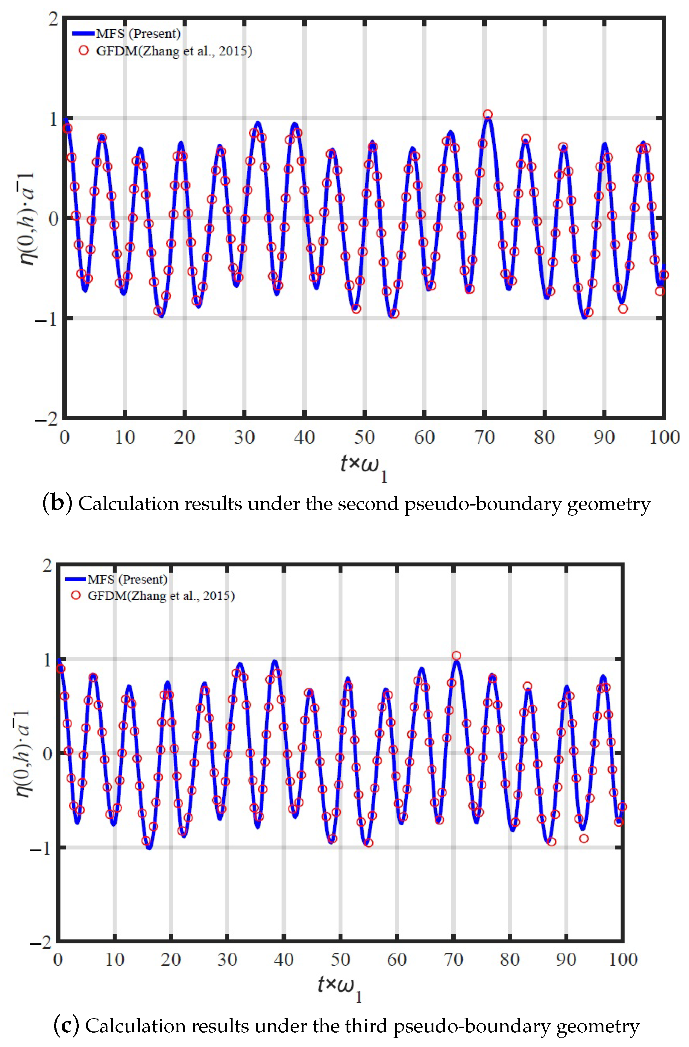
Figure 2 illustrates the schematic diagram of the MFS. The boundary nodes are arranged on physical boundaries, and the source nodes are arranged on a pseudo-boundary outside the computational domain. The fundamental solution of the Laplace equation is defined as [
20,
21,
22]:
where
is the distance from any boundary nodes
, where
, to the source nodes
, where
. It can be expressed as:
Since the boundary conditions already satisfied the governing equation, they could be expressed as a linear combination of the fundamental solutions with various weightings. Furthermore, the boundary condition is also known. Therefore, the weightings can be solved:
where
represents the weightings of
and
N denotes the number of source nodes.
Conventionally, the source nodes are fixed, and only the weightings are unknown. The number of boundary nodes is denoted by M, and it was set to be greater than or equal to the number of source nodes, i.e., .
However, in the current approach, the source nodes are free, which means that the parameter controlling the source position is unknown. Therefore, more boundary nodes are required to ensure that the number of equations is at least as large as the number of unknowns. Two schemes were proposed to allocate the source nodes. The boundary nodes are denoted by , where , and , where . Here, represents the physical boundary of the NWT.
In Scheme 1, the source node is defined as
, where
:
where
denotes the coordinates of the center of the domain. The unknown parameter
controls the magnification of the distance of the node
from the center of the domain. The rules for laying out the nodes should satisfy
.
In Scheme 2, the source node is defined as
, where
:
where
is a set of column vectors that give
, a unique parameter controlling the distance between the source
and the node
. Since a total of
unknown quantities are introduced, the deployment method should satisfy
.
In addition, it was assumed that the weightings are known and the initial values are zero. The initial values of the parameters
and
, which denote the normal distance between the physical and pseudo-boundaries, were set to 2.0. The numerical solution can be obtained from the linear combination of the fundamental solutions with various weightings. If these solutions are incorrect, a corrective action should be taken. The MATLAB© routine lsqnonlin was used to analyze the following discretized nonlinear equation system:
and the routine lsqnonlin was used to converge
, where
, to 0. In this process, the computational program iterates until the convergence criterion is reached. The options of lsqnonlin that were set are displayed in
Table 1. At the end of the lsqnonlin iteration, the approximate values of the weightings
and the parameter
or
are obtained. The parameters
and
are updated adaptively with lsqnonlin, meaning that the pseudo-boundary moves with each iteration.
3.2. Time Marching
In order to solve Equations (
1)~(
6), the second-order Runge–Kutta method was used to perform the time marching of
and
. This method provides second-order accuracy in time. Since Equations (
2) and (
3) are time-independent, the second-order Runge–Kutta method were used to update the free surface boundary Equations (
5) and (
6) as follows:
where
and
represent the velocity potential and free surface elevation at the
th time step, respectively, while
and
represent the velocity potential and free surface elevation at the
nth time step, respectively. Additionally,
and
can be expressed as follows:
where
and
can be expressed in a similar form as
and
:
In Equations (
17)~(
20), variables
,
, and
can be gained through the following expressions.
In Equation (
21), the first term of
is obtained using the forward difference scheme, the last term is obtained using the backward difference scheme, and the remaining terms are obtained using the central difference scheme. In Equation (
22),
denotes the square of the distance between the boundary node and the source node, where
m is the number of boundary nodes and
n is the number of source nodes. Here,
represents the normal vector of the free surface and
denotes the previously obtained weighting coefficients.
To stabilize the solution, ninth-order polynomials were used to fit the free surface, dynamic, and kinematic boundary conditions. The coefficients of the ninth-order polynomials were determined using the least-squares method. The form of a ninth-order polynomial is as follows (The flowchart of the proposed meshless numerical scheme for solving sloshing phenomena is presented in
Figure 3.):
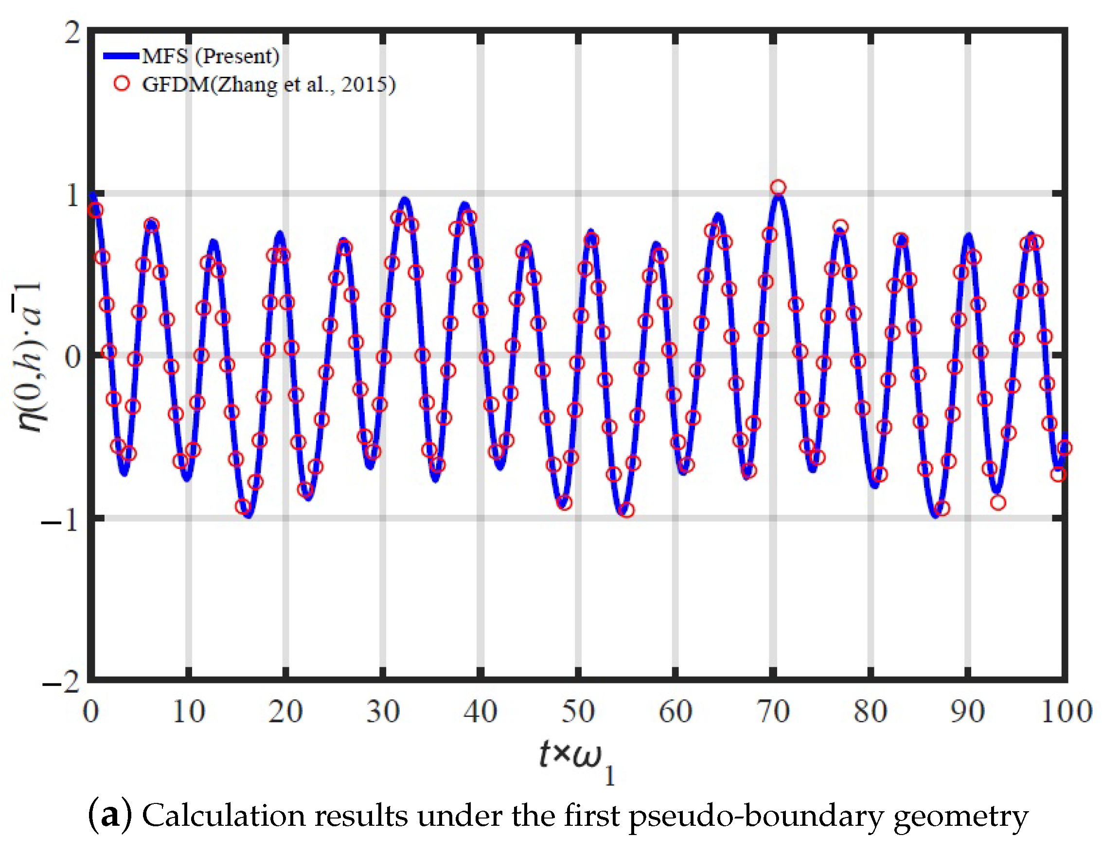
5. Conclusions
In this study, a meshless method was proposed to simulate sloshing in a 2D rectangular NWT. The second-order Runge–Kutta method and the MFS, based on moving pseudo-boundaries, were implemented for temporal and spatial discretization, respectively. The second-order Runge–Kutta method guarantees the accuracy and stability of dynamic and kinematic free surface boundary updates. The MFS, a meshless method with easy programming and high computational accuracy traits, was responsible for dealing with the Laplace equation at each time step. This study treated the position of the source nodes as an unknown variable to be solved simultaneously with the weighting coefficients, which avoided the need for fixing the position of the source nodes. This enabled adaptive calculations and improved the stability of the calculations and the numerical methods. The solution of the Laplace equation can be obtained easily by combining weighting coefficients and the fundamental solution. Meanwhile, the parameters and were adaptively updated using lsqnonlin.
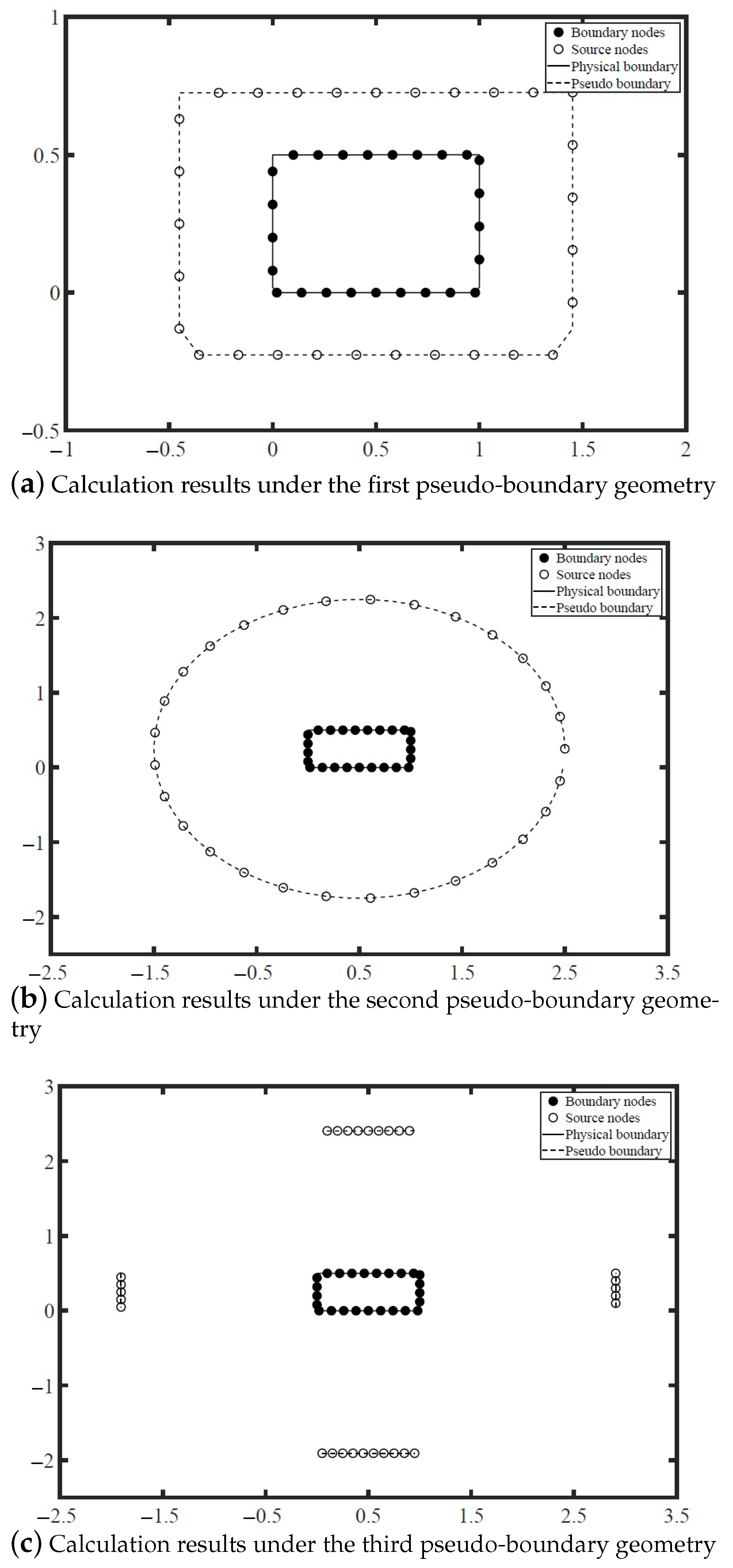
Three numerical simulations were analyzed to verify the accuracy and stability of the proposed numerical method. The numerical results were compared to other works. Through the convergence study of the number of nodes and time steps, the MFS based on the least-squares algorithm reported good computational stability and accuracy with fewer collocation nodes and a larger time step. Besides that, the geometry of the pseudo-boundary could affect the computational efficiency of the calculation. Likewise, the computational efficiency of the circular pseudo-boundary was approximately twice that of the boundary-dependent type. The main contribution of this study was expanding the application of the MFS in engineering by integrating it with the optimal configuration problem of pseudo-boundaries to solve practical engineering problems. The research in this paper showed that the MFS we proposed has great potential to be applied to other related marine engineering problems.
In this study, the time increment was assumed to be a constant number. Moreover, the arrangement of the source nodes was still relatively fixed in this study, and only the normal distance was adjusted. In principle, the source nodes can be arranged arbitrarily outside the computational domain, prompting future research to examine the effect of source node positioning on computational efficiency. The findings from this study indicated that the MFS can accurately calculate the nonlinear free surface in 2D sloshing and can be applied in other related studies.


