A Machine-Learning-Based Method for Ship Propulsion Power Prediction in Ice

Abstract

In recent years, safety issues respecting polar ship navigation in the presence of ice have become a research hotspot. The accurate prediction of propulsion power plays an important role in ensuring safe ship navigation and evaluating ship navigation ability, and deep learning has been widely applied in the field of shipping, of which the artificial neural network (ANN) is a common method. This study combines the scientific problems of ice resistance and propulsion power for polar ship design, focusing on the design of an ANN model for predicting the propulsion power of polar ships. Reference is made to the traditional propulsion power requirements of various classification societies, as well as ship model test and full-scale test data, to select appropriate input features and a training dataset. Three prediction methods are considered: building a radial basis function–particle swarm optimization algorithm (RBF-PSO) model to directly predict the propulsion power; based on the full-scale test and model test data, calculating the propulsion power using the Finnish–Swedish Ice Class Rules (FSICR) formula; using an ice resistance artificial neural network model (ANN-IR) to predict the ice resistance and calculate the propulsion power using the FSICR formula. Prediction errors are determined, and a sensitivity analysis is carried out with respect to the relevant parameters of propulsion power based on the above methods. This study shows that the RBF-PSO model based on nine feature inputs has a reasonable generalization effect. Compared with the data of the ship model test and full-scale test, the average error is about 14%, which shows that the method has high accuracy and can be used as a propulsion power prediction tool.

1. Introduction

The propulsion power requirements of polar ships in icy water are higher than those of ships in open water. Generally speaking, if the overall design of the same type of ship structure meets these requirements, the greater the propulsion power and the stronger the icebreaking capacity. However, choosing a larger propulsion power system increases the cost of shipbuilding, and such propulsion systems are relatively low in efficiency. Moreover, the propulsion system usually takes up more space on the ship. Therefore, reasonable prediction of the propulsion power for a polar ship is an important issue and deserves further study.

The propulsion power of a polar ship mainly depends on the ice resistance of the hull. Lindqvist [1] proposed a semi-empirical formula by summarizing full-scale measurements, model tests, and numerical calculations to predict the ice resistance. Semi-empirical formulas play an important role in ice resistance prediction, but the application is limited by ship form and environmental conditions. The usage of the formulas relies excessively on real ship experimental data, which cannot fully consider the influence of ship form, ice conditions, and other key factors. Taking account of the cost of full-scale testing and model testing, numerical methods are a good alternative for computing ship ice resistance. However, they rely on understanding the mechanisms of ice–ship interactions and include several simplifications and assumptions [2]. Sun et al. [3] designed a reliable ice resistance prediction ANN model within the set parameter range by selecting appropriate ship and ice parameters.

Currently, the propulsion power of polar navigation ships is mainly calculated based on the recommendations of various classification societies [4,5,6,7]. The propulsion power requirements of the classification societies under the IACS are based on the FSICR. Ding et al. [8] proposed a modified formula based on the FSICR to calculate the minimum propulsion power of polar ships. MAN Diesel A/S [9] compared various sizes of oil tankers and proposed that the power required by the FSICR is much higher than the power of ships that are equipped conventionally, and the power required by a 1A ice-class Aframax tanker is almost equal to the power of a main engine normally equipped with a VLCC.

The ABS (2010) also believes that the main engine power required by the Finnish–Swedish specification is too high. Other classification societies, such as the RMRS, CASPPR, and CCS, have formed power evaluation systems.

ANNs have been widely used in the field of ocean engineering in recent years. Kim et al. [10] considered the ice resistance in level ice and built an ANN model from the perspective of different feature inputs, but it is also possible to optimize the model structure and consider enriching the selection range of ship and ice parameters. Theodoropoulos et al. [11] predicted a ship’s propulsion power using different deep learning models, proposing a time series prediction model with high prediction accuracy and further improvement in the utilization of computational resources. Pedersen and Larsen [12] adopted ANN models under four different loading conditions to predict a ship’s propulsion power using three data sources for training and prediction; however, due to the lack of sufficient noon reports, the model had certain limitations when processing noon report data at the same time. In addition, compared with the limitations of traditional models in dealing with large datasets with significant variations, ANNs and deep learning are promising alternatives. In terms of visual recognition, Luo et al. [13] proposed a method based on an ANN for extracting fish information; the method had better robustness and higher accuracy compared to traditional visual algorithms. In terms of data processing, Ehsan et al. [14] proposed a novel deep-learning-based forest change method. Compared with other traditional U-Net-based models, deep learning methods better preserve forest changes and their set details, and they have great potential for providing quantitative and qualitative results.

In this work, an ANN model is proposed that is based on the selection of different features and algorithms where the feature selection includes ship, ice, and propeller parameters. We find that the ANN has good nonlinear mapping ability and good generalization ability when dealing with nonlinear data. Compared to traditional full-scale and model tests, the ANN is more efficient in terms of time and computation resources. Compared with R/V Sikuliaq full-scale experiments [15], PSV model experiments [16], and polar carrier model experiments [17], the ANN model prediction results have stability, reliability, and high prediction accuracy.

2. ANN Models

Machine learning methods can be used as a tool to tackle complicated problems. They can address different problems such as function approximation, classification, and regression. The ANN is one of the most commonly used methods in the field of machine learning. Its network structure is mainly composed of neurons, layers, and networks [18]. Although the function of a single neuron is limited, an ANN composed of multiple neurons is highly effective in solving problems. The trained ANN model is represented by a set of algorithms that are trained using input datasets to identify a good hypothesis function for the target issue. This has proven to be a feasible and practical approach to solving highly nonlinear problems.

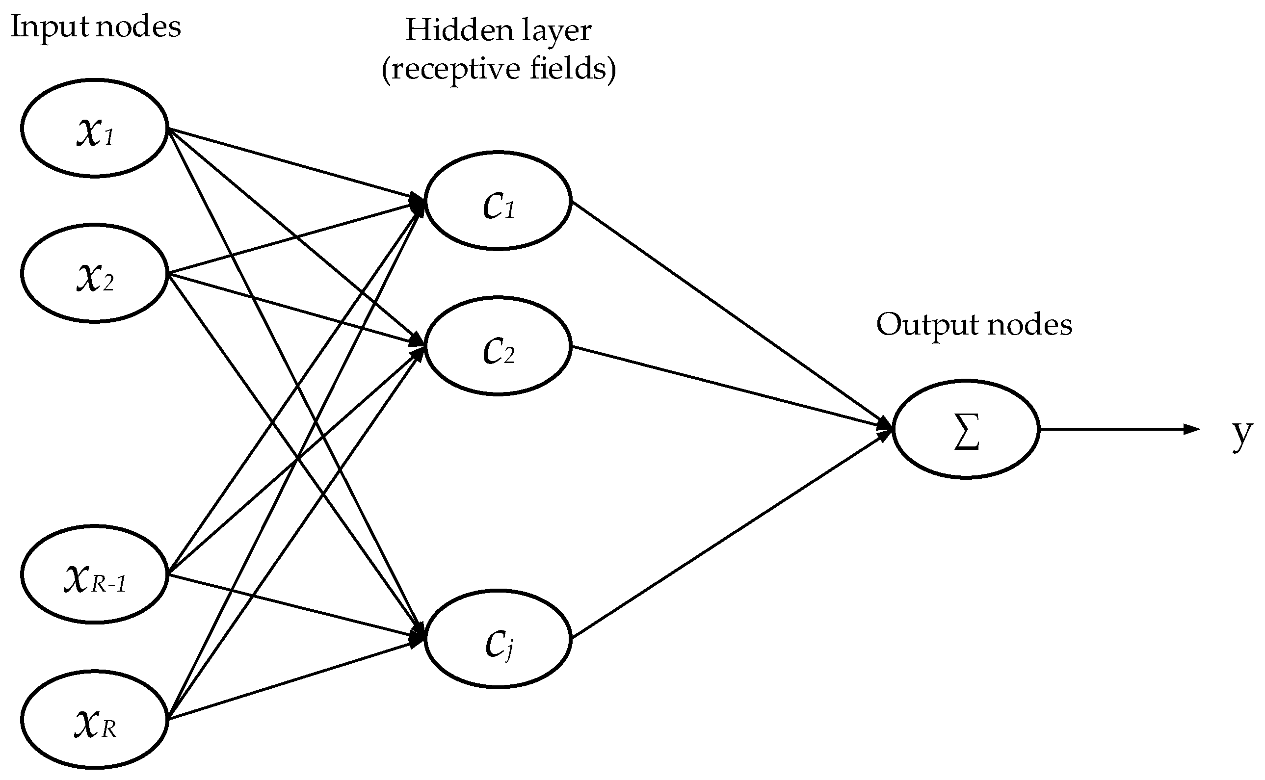
A three-layer feed-forward neural network (RNNM) is proposed herein, as shown in Figure 1. In the FNN, there is no feedback from the latter layer to the former layer, and each layer’s neurons come from the former layer’s input. Neuron c in the hidden layer of the network is a linear combination of the input feature x multiplied by the weight matrix and the deviation vector. The output is a linear combination of hidden layer neurons.

In the RNNM, the input includes ship, ice, and propeller parameters, while the output is propulsion power. The sigmoid function is selected as the activation function on the hidden layer neurons, and the Levenberg–Marquardt algorithm is taken as the training function of the network. The convergence speed of the Levenberg–Marquardt algorithm is relatively slow, but it still has good generalization effects on the training set with less sample data.

3. Propulsion Power Requirement of Classification Societies

Ship propulsion power in ice-covered waters can be estimated using the propulsion requirements of various classification societies. At present, propulsion power requirements mainly refer to the FSICR. To select the appropriate input characteristics, the propulsion power calculation formulas of different classification societies can be referred to.

The FSICR [19] is widely used for vessels in the Northern Baltic Sea in winter. The propulsion power requirements are based on the total resistance of ships in first-year ice. The FSICR presents a formula for calculating the minimum propulsion power under different ice classes, and the power is calculated as a function of the thrust. Three methods are used to obtain thrust, namely, the CFD method, the bollard pull test, and the towing test at low speed [20].

The propulsion power equations provided by the CCS [21] are formulated with a set of empirical coefficients. These coefficients are divided based on the propulsion type of the propeller, which includes the angle between the stem and the waterline, ship breadth, ship length, ship velocity, and ice thickness.

The RMRS assigns the ice class of icebreakers into the categories Ice2 to Arc9, and it provides calculation methods for the minimum propulsion power requirements under different ice classes. The propulsion power is linearly related to the displacement. For ice-strengthened vessels under ice classes Ice2 and Ice3, the displacement required by the minimum propulsion power should not be more than 8000 m³.

The ABS proposes that propulsion power can be calculated using the bollard pull test. Ice-going ships should meet ice class PC1–PC7, and the power received by the propeller under the maximum power should satisfy the continuous icebreaking mode.

The minimum power formula suggested by the CASPPR is a function of displacement and ship width at the waterline. This set of functional relationships is based on a set of empirical coefficients derived from different ice class conditions. It should be noted that the final power calculated should not be less than the power of the ship sailing at 12 knots in still water.

These five formulas have introduced propulsion power specification requirements from various classification societies, where the main parameters that influence propulsion power are given. The important parameters are summarized in

Table 1. Parameters used in propulsion power formulas of classification societies.

	Item	Notations	Unit	FSICR	CCS	RMRS	ABS	CASPPR	Occurrence (Total 12)
Ship-related parameters	Ship speed	$v$	m/s		√				1
	Ship length	$L$	m	√	√				3
	Ship breadth	$B$	m	√	√	√	√	√	5
	Ship draught	$T$	m	√	√		√		3
	Bow length	$L_{bow}$	m	√					1
	Parallel mid-body length	$L_{par}$	m	√					1
	Waterline angle	$\beta$	°	√	√		√		3
	Trim angle	$\phi$	°	√		√	√		3
	Average bow flare angle at waterline	$\psi$	°				√		1
	Entry angle at waterline	$\partial$	°				√		1
	Stem angle	$\varphi$	°		√				2
	The rake of the stem at the centerline	${\phi }_1$	°	√					1
	The rake of the bow at B/4	${\phi }_2$	°	√					1
	Area of the waterline of the bow	$A_{WF}$	m2	√					1
	Displacement	$\Delta$	m3		√	√	√	√	4
Ice-related parameters	Ice thickness	$h$	m	√	√	√	√	√	5
	Snow thickness	$h_s$	m		√				1
Propeller-related parameters	Propeller diameter	$D_P$	m	√			√	√	3
	Propeller number	$Z$	-	√			√	√	3
	CPP/FPP	$f$	-	√	√	√			3
	Number of constants	-	-	1	4	4	3	1	/

. As shown in Table 1, there are 15 ship-related parameters, 2 ice-related variables, and 3 propeller-related parameters selected to predict the propulsion power. Some parameters show a high occurrence, and some are low in the existing formulas. Sun et al. [3] explained the main factors affecting ice resistance in the semi-empirical formula in detail. Based on the ANN-IR, the appropriate propeller parameters are added to predict propulsion power in this paper. The schematic diagram of all angles is defined as shown in Figure 2.

4. Database for ANN Training

To select the dataset and determine key features is important when training a neural network model. Different datasets derived from model-scale and full-scale tests are used in the RNNM to train the network. The appropriate dataset is selected for feature analysis. The results are then compared with the actual propulsion power of the R/V Sikuliaq ship from Neville and Martin [15].

4.1. Database Preparation

In this study, the dataset is sourced from 13 different full- and model-scale tests with a total of over 140 sets of data. Among them, the experimental data comprise 123 sets with the rest comprising design power data. Dataset [4,17,22,23,24,25,26,27,28,29,30,31] selection is shown in

Table 2. Construction of propulsion power ANN model data source.

Ship Name	Reference	Test Conditions	Power Condition	Ice Condition
A polar carrier	(Ji et al., 2018)	Model-scale	Actual	Level ice
USCG	(Wang et al., 2018)	Model-scale	Actual	Level ice
KV Svalbard	(Madsen, 2010)	Full-scale	Actual	Level ice, etc.
R class	(Spencer and Jones, 2001)	Full-scale	Actual	Level ice
29 polar icebreakers	(Cao, 2020)	Full-scale	Actual	Level ice
Araon	(Kim et al., 2011)	Full-scale	Actual	Level ice
Envik Kemira Link Star Solano Atserot Sotka Finnoak Aila Finnmerchant Futura Arkadia Sirius Windia Nossan Shuttle	(Juva and Riska, 2002)	-	Design	Level ice
KV Svalbard	(Jeong et al., 2017)	-	Design	Level ice
Akadenilk Fyodorov	(Zhang et al., 2017)	-	Design	Level ice, etc.
Tor Viking II	(Su et al., 2010)	-	Design	Level ice
Araon	(Kim et al., 2011)	-	Design	Floating ice
MT Uikku	(Zhou et al., 2018)	-	Design	Level ice
A general cargo ship	(Montewka et al., 2013)	-	Design	Level ice/ice ridge/ice compression

Note: the test with an ice thickness of 1.3 m is selected as the training data, and the test with an ice thickness of 1.6 m is selected as the verification data (Ji and Tian, 2018).

. The model test data are amplified to full-scale data based on the specific scale factors that are given in the experiment, and the conversion relationship is shown in

Table 3. Similarity relations for ship model test in ice.

Property	Scale Factor	Property	Scale Factor	Property	Scale Factor
Length	$\lambda$	Ice thickness	$\lambda$	Propeller diameter	$\lambda$
Breadth	$\lambda$	Flexure strength	$\lambda$	Propeller number	1
Draught	$\lambda$	Density of ice	1
Stem angle	$1$	Friction coefficient	1
Velocity	${\lambda }^{1/2}$
Waterline angle	$1$	Ice resistance	${\lambda }^3$	Propulsion power	${\lambda }^{3.5}$

.

4.2. Propulsion Power Prediction Using Different Databases

Sun et al. [3] verified the feasibility of constructing an ANN using model test results as training data and full-scale test results as validation data. In this study, since the full-scale and model tests have limited data sources, ship design power data are added, and some parameters are added referring to the power calculation requirements from classification societies. For example, the power requirement in the FSICR notes that the ship speed in channels of a given thickness is at least 5 knots [4]. The full-scale test and model test data are used as a set named Dataset-1. On this basis, the ship design power is added as a set named Dataset-2. To select appropriate training data, the reliability of the dataset is verified in RNNM construction.

In the RNNM, the dataset is divided into three parts: training, verification, and testing. Among these, the training set is used to train the model, the verification set is used to adjust the super parameters of the model, and the test set is used to evaluate the accuracy and generalization ability of the model. In regression analysis, one of the most important indicators to judge the quality of the dataset is the size of the R-value of the test set.

The square root of the determination coefficient (R) of the two models trained based on Dataset-1 and Dataset-2 is shown in Figure 3 and Figure 4, where the abscissa represents the target output, and the ordinate represents the fitting function between the predicted output and the target output. The value of R in the interval [0, 1] is used to indicate the correlation between prediction and output data. The relationship between prediction and output becomes more random as the R-value approaches 0, and the correlation between them is stronger as the R-value approaches 1. The R-value in Dataset-1 is generally lower than that in Dataset-2, but the generalization ability of the model is mainly judged by the R-value of the test set. The test set based on Dataset-1 fits well, and the R-value is much higher than that of Dataset-2. However, the R-value is used to analyze the correlation between prediction and output, which can be used as a reference, but a model cannot be judged only by the size of the R-value. In model training, verification, and testing, if the R-value is not high, the reason may be the lack of fitting caused by less data and insufficient features. In the case of less data, the reason for the high R-value may be that the feature variables contain the features of strong correlation of dependent variables or it may be the over-fitting caused by model training.

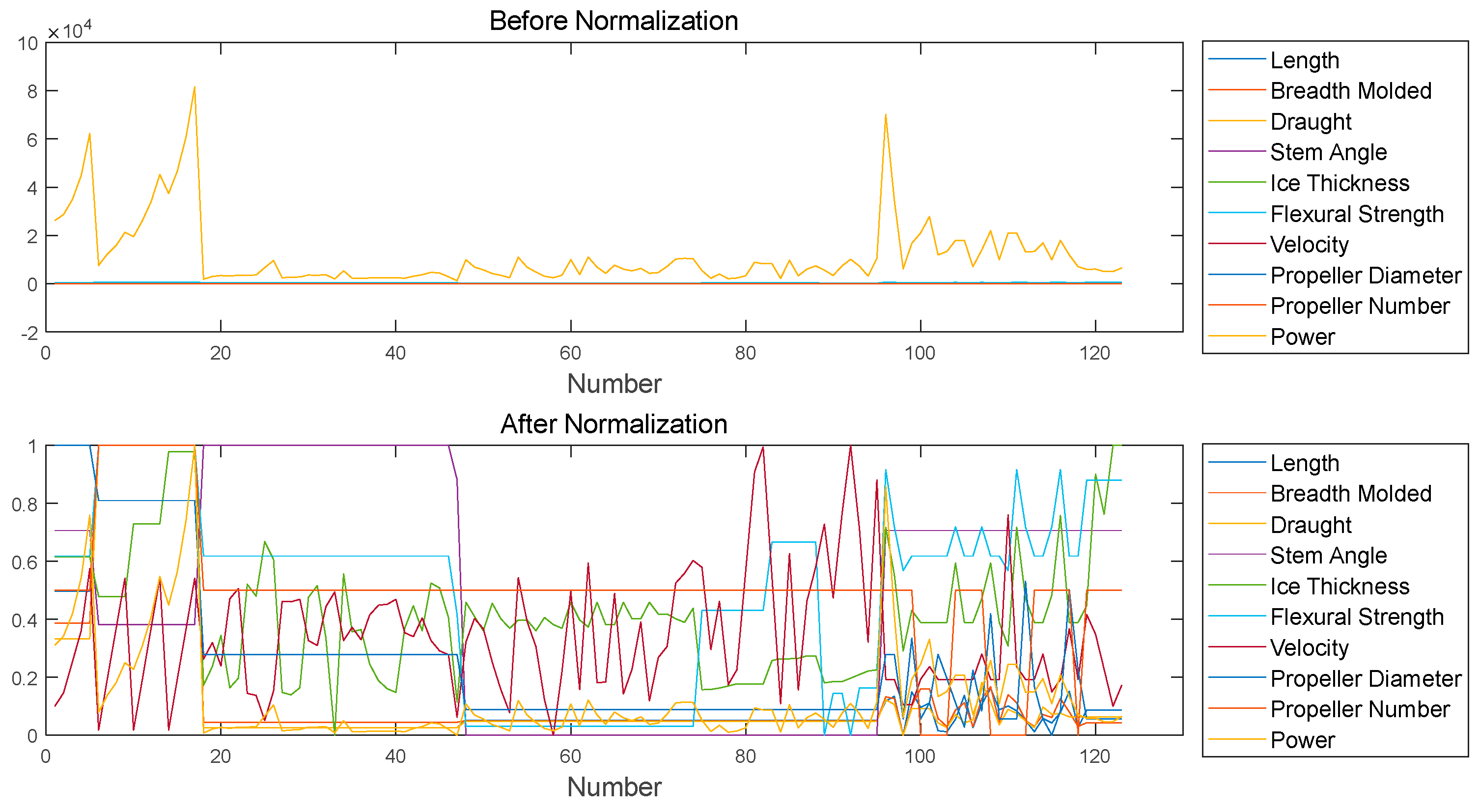
To keep the weights of each feature on the same scale and eliminate the dimensional influence between features, normalization is used to linearly transform the training dataset to the range [0, 1]. In Figure 5 and Figure 6, the abscissa represents the number of the training dataset, and the ordinate represents the value range of the training dataset. From the data normalization, it can be seen that the input and output features before normalization are not in the comparable range, and the input features affect each other, but there is no correlation between the propulsion power and the input features. After normalization, the features are in the same order of magnitude, with the input and output features affecting each other. Feature scaling can improve the prediction and convergence speed of the ANN model, but the maximum value needs to be redefined when new data are added. The formula is as follows:

$$z^{\prime }=\frac{z-z_{\min }}{z_{\max }-z_{\min }}$$

(1)

where $z_{\min }$ and $z_{\max }$ represent the minimum and maximum values of one feature, respectively; and $z$ and $z^{\prime }$ represent data before and after normalization, respectively.

The R/V Sikuliaq is an icebreaking research vessel [15], and its full-scale trials were conducted in the Bering Sea in March and April 2015. The RNNM uses two different datasets to predict the propulsion power of the vessel R/V Sikuliaq. The results are compared with predictions from the FSICR. The ice resistance value of the FSICR is based on the prediction result of the ANN-IR, and this power prediction is defined as ANN-IR-FSICR. The parameters of R/V Sikuliaq are shown in

Table 4. R/V Sikuliaq main dimensions.

Length (m)	Breadth (m)	Draught (m)	Stem Angle (°)	Flexural Strength (kPa)	Ice Thickness (m)	Velocity (m/s)	Propeller Diameter (m)	Propeller Number (-)
79.705	15.85	5.944	30	250	0.2–0.47	2.2–5.5	4	2

. The ice resistance and propulsion power under different ship speeds are shown in Figure 7. The formula for calculating the propulsion power of the FSICR is as follows:

$$P=K_e\frac{{\left(R_{CH}/1000\right)}^{3/2}}{D_P}$$

(2)

where $P$ is the propulsion power; $R_{CH}$ is the ice resistance, applicable to the calculation of ice resistance in ice channels with broken ice and solid ice layers; $D_P$ is the diameter of the propeller; $K_e$ is the coefficient related to the propeller, mainly used for traditional propulsion forms; and the specific coefficients are shown in

Table 5. Calculation coefficients of propulsion power.

Propulsion Mode	CPP	FPP
Single screw	2.03	2.26
Twin screw	1.44	1.60
Three screw	1.18	1.31

.

In Figure 7, the ice resistance predicted from the ANN-IR model increases with the increase in ship speed. This conforms to the general rule. In propulsion power prediction, the ANN-IR-FSICR prediction method has an average error of 24.6%; when the ship speed is 5.5 kn, the predicted value is about 50% more than the actual value. Predictions-1, which are based on Dataset-1, have an average error of 37.2%, and Predictions-2, which are based on Dataset-2, have an average error of several times. Considering the three prediction methods under different ship speeds, it can be seen that the ANN-IR-FSICR is the lowest among the three models, and Predictions-1 and Predictions-2 overestimate the results. In addition, the R/V Sikuliaq icebreaker also undergoes propulsion power experiments under different ship speeds and ice thicknesses, as shown in

Table 6. Prediction of propulsion power using ANN model under four working conditions.

Item	Unit	Case1	Case2	Case3	Case4
h	m	0.30	0.34	0.33	0.47
v	m/s	2.5	2.4	3.2	2.2
Measurements	kW	1208	1208	1835	1857
Predictions (ANN-IR-FSICR)	kW	1302	1352	1533	1880
Predictions-1	kW	2741	2910	1969	2842
Predictions-2	kW	9772	10,028	8724	8724

.

The three model predictions under the four working conditions summarized in Table 6 are plotted in Figure 8. The ANN-IR-FSICR is relatively close to the measurement, with average errors between 1.2% and 16.4%, and the average error is 9.3%. The average error of Predictions-1 is close to twice as high as the measured value. The prediction result of Predictions-2 is the largest, and its predicted value is several times the measured value.

The reason for these results is that the value of the design power itself is not consistent with the measured value, e.g., the design power of the same polar oil tanker is 32,000 kW when the ice thickness is 1.5 m, and the velocity of ship is 5 kn, and the actual propulsion power under the same working conditions is around 45,000 kW (Zhou and Ding, 2020). In the next step, Dataset-1 is used as the training data. Considering its simple structure and large prediction error when dealing with sophisticated nonlinear data, the RNNM is only used to select the dataset.

4.3. Feature Scaling

The Pearson correlation coefficient is introduced to visualize the correlation between input $x$ and output $y$ [32]:

$${\rho }_{x,y}=\frac{\mathrm{cov}\left(x,y\right)}{{\sigma }_x{\sigma }_y}=\frac{E\left(\left(x-{\mu }_x\right)\left(y-{\mu }_y\right)\right)}{{\sigma }_x{\sigma }_y}=\frac{E\left(xy\right)-E\left(x\right)E\left(y\right)}{\sqrt{E\left(x^2\right)-E^2\left(x\right)}\sqrt{E\left(y^2\right)-E^2\left(y\right)}}$$

(3)

where the Pearson correlation coefficient is represented by ${\rho }_{x,y}$, the covariance of variables x and y is represented by $\mathrm{cov}\left(x,y\right)$, the standard deviation of variables x and y is represented by ${\sigma }_x$ and ${\sigma }_y$, and the mathematical expectation is represented by E; both x and y are normalized.

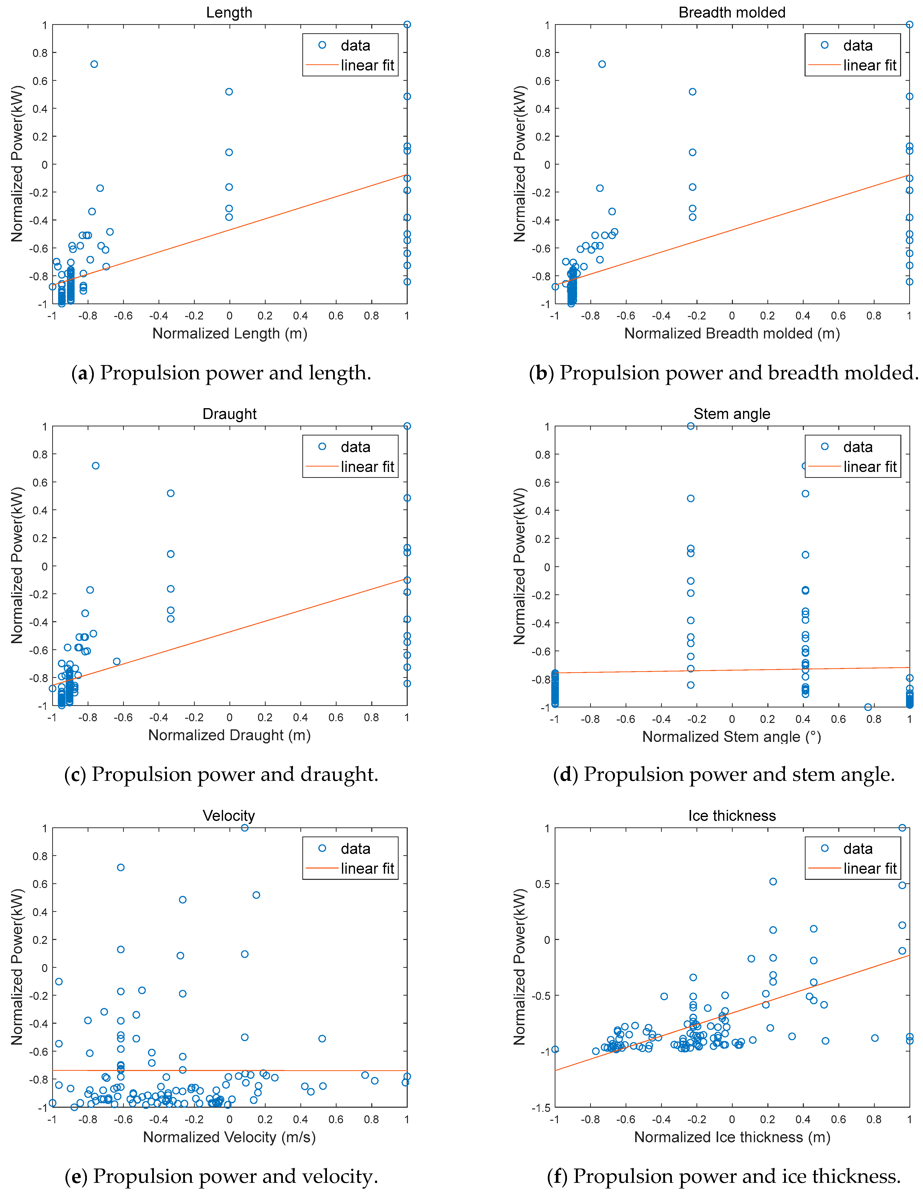
The linear relationship is shown in Figure 9. Figure 9a–i shows the Pearson correlation coefficients between the ship length, breadth molded, draught, stem angle, velocity, ice thickness, flexural strength, propeller diameter, and propeller number and the propulsion power, respectively. The correlation (linear fitting) between the nine features (ship, ice, propeller) and the output is evaluated within [−1, 1] after normalization of the training dataset, where +1 and −1 stand for strong positive and negative correlation, respectively, and 0 represents no correlation.

In the FSICR, the calculation of propulsion power is based on the ice resistance value, and accurate ice resistance prediction is the premise of calculating the propulsion power. Our study of the ANN-IR shows that the ANN model has excellent generalization ability and can be used as a reliable and accurate tool for ice resistance prediction compared with the traditional full-scale test, model test, and semi-empirical formula in polar ship design. According to the calculation formula of propulsion power in the FSICR, two features, propeller diameter and propeller number, are added based on ANN-IR feature selection.

The linear correlation (Pearson correlation coefficient) between each feature and the propulsion power can be seen in

Table 7. Selected input variables for the ANN.

Category	Input	Notations	Unit	Pearson Correlation Coefficient	Range
Ship parameters	Length	$L$	m	0.3966	79.6–440.5
	Breadth	$B$	m	0.3947	15.85–88.5 (m)
	Draught	$T$	m	0.3826	5.715–36 (m)
	Stem angle	$\varphi$	°	0.0195	18–35 (°)
	Velocity	$V$	m/s	−0.0007	0–12 (knots)
Ice parameters	Ice thickness	$h_i$	m	0.5171	0.2–2.5 (m)
	Flexure strength	${\sigma }_f$	kPa	0.2339	208–690 (kPa)
Propeller parameters	Propeller diameter	$D_P$	m	0.4169	3.8–7.4 (m)
	Propeller number	$Z$	-	0.2454	1–3 (-)

. This shows that ice thickness, ship length, ship width, draught, propeller diameter, and propeller number are highly correlated with propulsion power, while the flexure strength, stem angle, and velocity are less dependent on the propulsion power.

In feature correlation analysis, there is a high degree of dispersion between inputs and outputs, mainly due to the Pearson correlation coefficient being sensitive to the linear relationship between the two variables, while the input variable and propulsion power are nonlinear. In addition, the sample data selection is dependent on the experimental environment, and the quality of sample data directly affects the dispersion between the two variables.

The Pearson correlation coefficient is the covariance ratio of the standard deviation, which is highly dependent on the database. In the construction of an ANN model, the first thing to consider is the quality of the database. There are several aspects that should be considered when using the database. First, under the IACS, the polar ship propulsion power requirements of each classification society have their own algorithms, which are not universal for ship tests under different working conditions. Secondly, during an experiment, the selection and recording of some parameters and data have a certain degree of subjectivity, and some factors may be idealized or ignored. One example is that the FSICR is aimed at the navigation area in the Baltic Sea, and the power calculation is based on the resistance performance requirements of each ship type in first-year ice, and the propulsion power may be overestimated when ships sail in other areas.

5. RBF-PSO Algorithm

An ANN model with better prediction accuracy and generalization effects needs to be considered due to the high prediction error between the prediction values of the RNNM and the ANN-IR-FSICR. In the ice resistance prediction model, RBF was introduced to construct the neural network model, and PSO was used to optimize the model. The results indicate that the RBF-PSO is a good algorithm model. Therefore, a prediction model of propulsion power based on RBF-PSO is proposed.

5.1. Propulsion Power ANN Overview

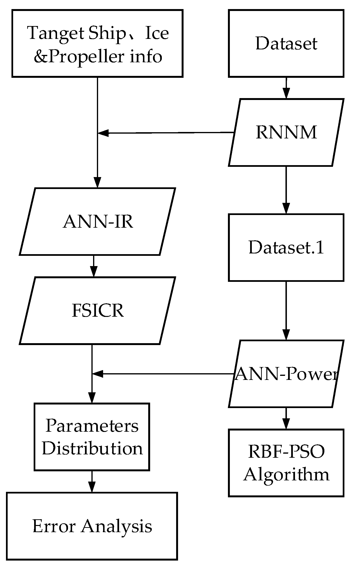
The propulsion power can be predicted for the target ship through the propulsion requirements of classification societies and the ANN model. The prediction of propulsion power using the ANN model is divided into two parts: prediction based on the ANN-IR and the FSICR, and direct prediction based on ANN-Power. The first part involves the indirect prediction of propulsion power. By using the ANN-IR proposed by Sun et al. [3] and combining it with the FSICR propulsion power calculation formula, the propulsion power of ships sailing in ice regions can be obtained. The second part involves directly predicting the propulsion power, establishing an RNNM model for dataset selection, and establishing an RPF-PSO model for the direct prediction of propulsion power. The final ANN model can be created by combining this with the parameter distribution. The process is illustrated in Figure 10.

5.2. RBF and PSO Algorithm

RBF is a three-layer feed-forward neural network. The basic idea is to use RBF to convert the input vector from a low-dimensional, linear, non-separable vector to a high-dimensional, linear, separable vector [33]. The commonly used activation function is a Gaussian function:

$$R\left(x-c\right)=\exp \left(-\frac{1}{2{\sigma }^2}{‖x-c‖}^2\right)$$

(4)

where the Euclidean norm is represented by $‖x-c‖$, the input sample is represented by $x$, the center of the Gaussian function is represented by $c$, and the variance of the Gaussian function is represented by $\sigma$.

The functional relationship of the output layer is represented as:

$$y_j={\displaystyle \sum _{i=1}^h{w}_{ij}R\left(x_p-c_i\right)}j=1,2,\cdots ,n$$

(5)

where the $pth$ input sample is represented by $x_p$, the center of the node of the network hidden layer is represented by $c_i$, the connection weight between the hidden layer and the output layer is represented by $w_{ij}$, the number of hidden layer junctions is represented by $h$, and $y_j$ is the actual output of the $jth$ output node of the network corresponding to the input sample.

When the training sample is ${\left\{\left(X_i,{\widehat{y}}_i\right)\right\}}_{i=1}^P$, the cost function for using LS is shown below:

$$\sigma =\frac{1}{P}{\displaystyle \sum _{i=1}^p{‖{\widehat{y}}_i-y_i‖}^2}$$

(6)

where $p=1,2,3,\cdots ,P$, $P$ is the total number of samples, ${\widehat{y}}_i$ is the expected output value, $y_i$ is the actual output of the $i\mathrm{th}$ output, and $\sigma$ is the variance of the basis function.

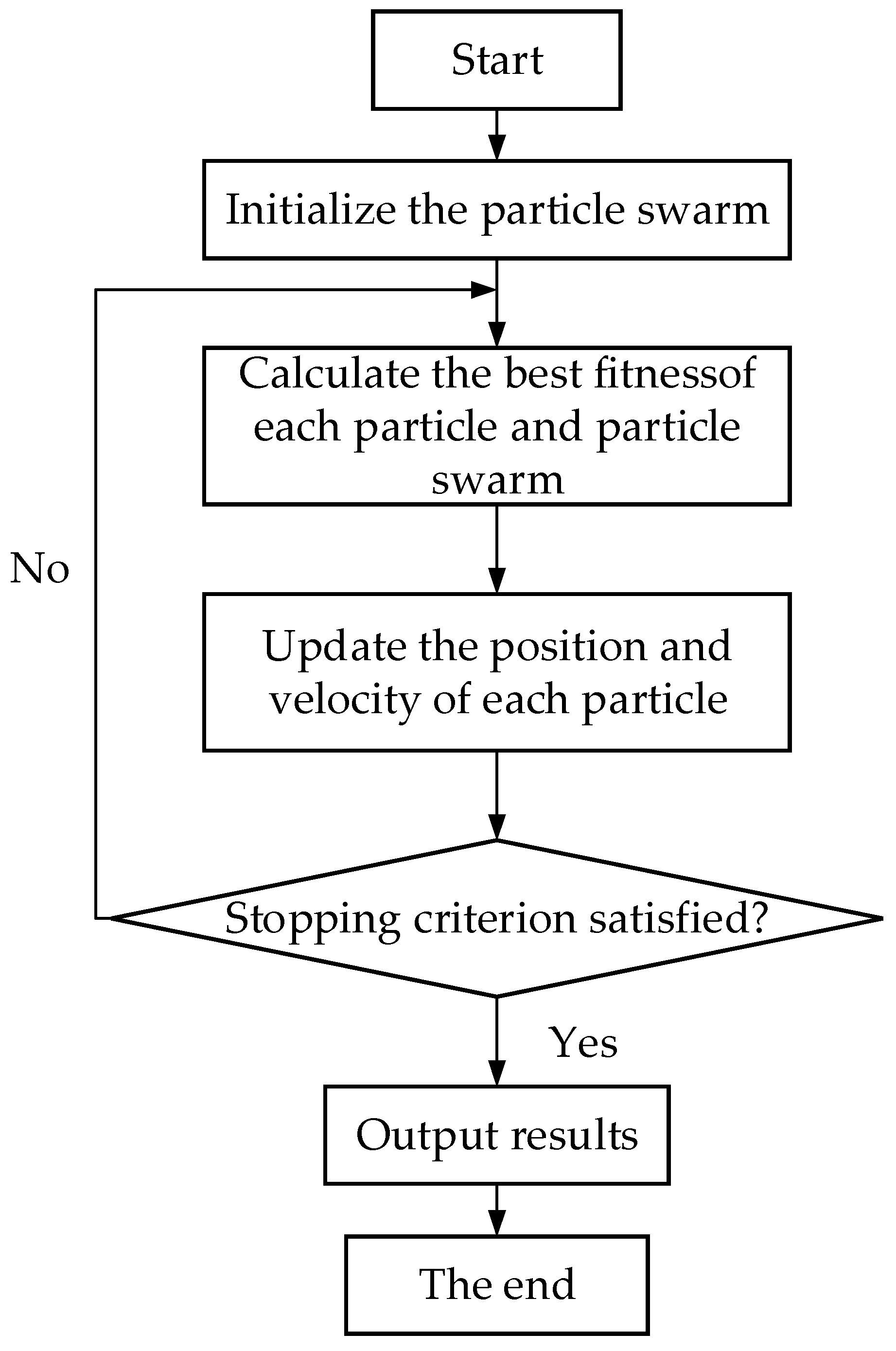
The PSO algorithm is an optimization algorithm of swarm intelligence which was first proposed by Eberhart and Kennedy in 1995 [34]. The basic idea of the PSO algorithm is to solve optimization problems through cooperation and information sharing among individuals in a group; that is, particles have the ability to learn and remember their own evolution and group evolution in order to find the optimal solution.

In PSO, each particle has a fitness value determined by an optimized function. The direction and distance of a particle flying in the problem space are determined using its assigned random speed [35]. Assume the population of particles in an n-dimensional search space is initialized with the random vector position $X_i=\left(x_{i1},x_{i2},\dots ,x_{in}\right)$ in the range of the dataset patterns and the velocity $V_i=\left(v_{i1},v_{i2},\dots ,v_{in}\right)$. Each particle keeps track of its coordinates in the problem space associated with the best solution (fitness). We define the fitness to determine whether a particle is close to the optimal solution. The particle moves in the solution space and updates the individual position by tracking the individual extreme pbest and the group extreme gbest. pbest refers to the best fitness position of particle Xi, and gbest refers to the best fitness position of the particle swarm. The above PSO optimization algorithm flow is shown in Figure 11.

In the global environment, the update equations for PSO velocity and position are shown below [36,37].

For the $i\mathrm{th}$ iteration:

$$v_{id}^k=w{v}_{id}^{k-1}+c_1{r}_1\left(pbes{t}_{id}-x_{id}^{k-1}\right)+c_2{r}_2\left(gbes{t}_d-x_{id}^{k-1}\right)$$

(7)

$$x_{id}^k=x_{id}^{k-1}+v_{id}^{k-1}$$

(8)

where $x_{id}^{k-1}$ is the velocity of particle $i$ at the ${\left(k-1\right)}^{th}$ iteration in d dimensions; $v_{id}^k$ is the updated velocity of particle $i$ at the $k^{th}$ iteration in d dimensions; $c_1$ and $c_2$ represent the acceleration factor in the interval [0, 2], which is used to adjust the inertial weight of local and social areas; $r_1$ and $r_2$ are uniformly distributed random numbers generated in the range [0, 1] [38,39]; and $w$ is the inertial weight, whose function is to control the influence of the velocity between particles.

The essence of PSO-optimized RBF is to replace the original gradient descent algorithm with the particle swarm algorithm on the basis of an unchanged model. Figure 12 is the schematic diagram of algorithm optimization, and the hyperparameters of the ANN model are listed in

Table 8. Hyperparameters of RBF-PSO ANN model.

Hyperparameters	Values
Hidden layer numbers	3
Hidden layer sizes	(40,20,10)
Loss function	MSE
Maximum number of iterations	1000
Learning rate	0.001
Number of initialization particles	100
Kernel function	Gaussian

.

The ANN model built in this study is a multi-input, single-output model. After the model is trained, parameters such as the variance coefficient and weight no longer change, and the output result is a numerical value that only changes with the input parameters. The results do not have randomness. After the parameters shown in Table 7 and used in Figure 13, Figure 14, Figure 15, Figure 16, Figure 17 and Figure 18 are optimized by the PSO algorithm, the functional relationship is as follows:

$$y=W\cdot \exp \left(-\frac{1}{2{\sigma }^2}‖X-b‖\right)$$

(9)

The input sample is represented by X, the center of the hidden layer node of the network is represented by $b$, the connection weight from the hidden layer to the output layer is represented by $W$, and the actual output of the network corresponding to the input sample is represented by $y$.

$$\sigma =1,W=\left[\begin{array}{lllll}-0.0220& -0.0217& 0.0211& 0.0205& \cdots \\ -0.1643& -0.2023& 0.2047& 0.1923& \\ 0.0220& 0.0216& -0.0210& -0.0205& \\ 0.0182& 0.0446& -0.0388& -0.0125& \\ 0.0226& 0.0201& -0.0198& -0.0210& \\ -0.0018& 0.0231& -0.0192& 0.0023& \\ 0.0219& 0.0227& -0.0220& -0.0204& \\ -\mathrm{0,1577}& -0.0170& 0.0258& 0.1219& \\ -0.0288& 0.0604& -0.0520& -0.0176& \\ -0.0021& -0.0880& 0.0827& 0.0270& \\ ⋮& & & & \end{array}\right],b=\left[\begin{array}{l}0.0202\\ 0.1445\\ -0.0201\\ -0.0964\\ -0.0194\\ -0.0446\\ -0.0204\\ 0.2078\\ -0.1650\\ 0.3746\\ ⋮\end{array}\right]$$

Here, $W$ is a $20*40$ matrix, and the numbers in $W$ are the matrix parameter values after the model training is completed; $b$ is a $20*1$ matrix.

6. Results and Validation

A polar carrier model test, R/V Sikuliaq full-scale test, and icebreaker PSV model test were selected to test and verify the ANN model. Trend and error analyses of propulsion power with different ship speeds and ice thicknesses were undertaken.

6.1. Polar Carrier (Model Scale)

A polar carrier model test was performed by Ji et al. [15]. The resistance prediction was based on the ANN-IR, and the propulsion power prediction of FPP and CPP was based on RBF-PSO, the FSICR, and the ANN-IR-FSICR. The corresponding results are plotted in Figure 13.

The model test mainly considers icebreaking and propulsion at low speeds. In Figure 13, the predicted ice resistance of the ANN-IR shows an obvious upward trend compared with the measured value after the ship speed of 1 m/s. In the ANN-IR training set, the maximum ice thickness is 1.5 m, and its prediction trend is affected by the training feature range to some extent. The error range between the predicted ice resistance and the measured value is 0.7–18.1%, with an average error of 7.8%. In propulsion power prediction, the average error between the predictions based on the RBF-PSO model and the FPP and CPP propulsion values is 14.1% and 22.3%, respectively. Based on the ANN-IR, the average errors between the FSICR and the FPP and CPP propulsion values are 48.6% and 56.6%, respectively. The average errors between the propulsion power calculated using the FSICR and the propulsion values of FPP and CPP are 68.2% and 47.5%, respectively. The error of the ice resistance predictions based on the ANN-IR is small, but the error between the predicted value and the measured value is high after the FSICR calculation. The error of the propulsion power prediction based on the ANN is the smallest, and the stability is the best. In addition, among the three methods for power prediction of the FPP and CPP propulsion modes, RBF-PSO has the smallest prediction error for the FPP propulsion mode, which is related to the large number of sample sets of the FPP propulsion mode in the training set.

6.2. R/V Sikuliaq (Full Scale)

The R/V Sikuliaq is an icebreaking research vessel, and its full-scale trials were conducted in the Bering Sea during March and April 2015. Figure 14 shows the model prediction results and full-scale measurements [13].

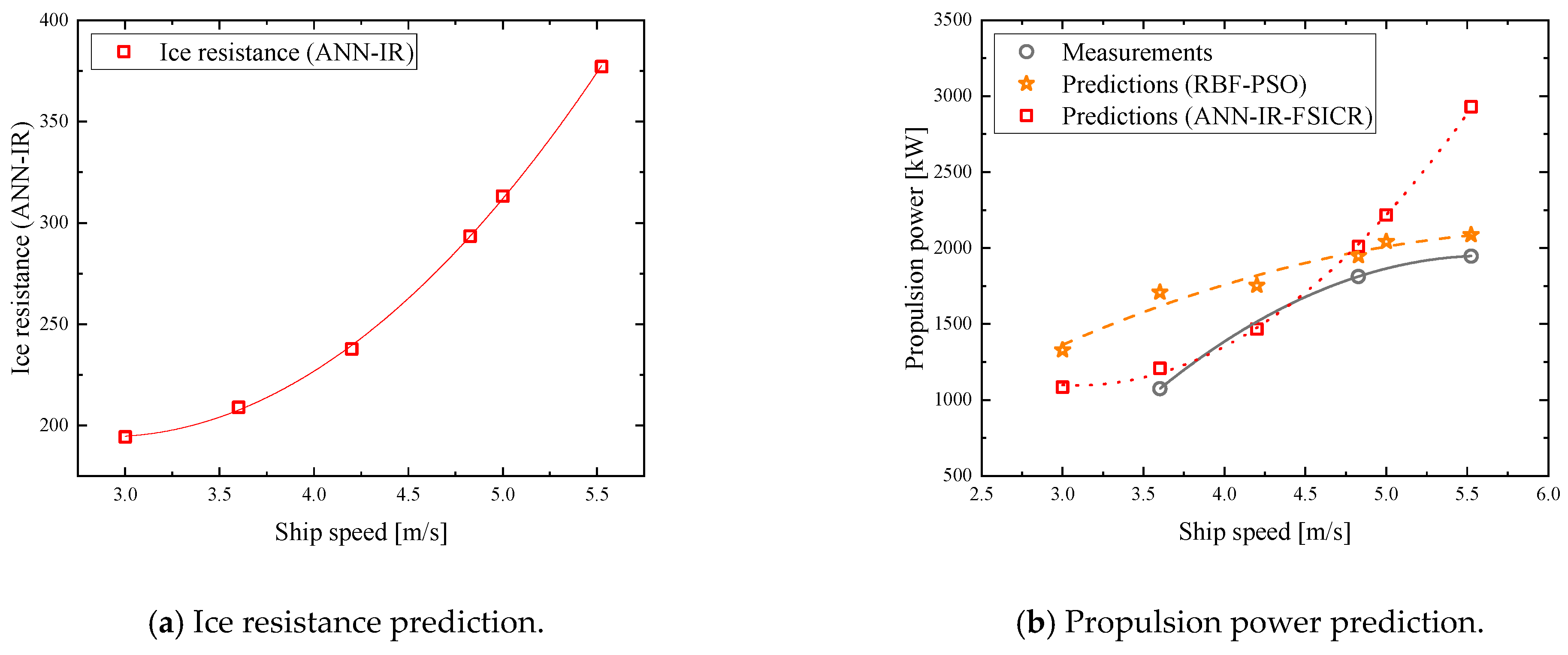
On the basis of Figure 7, the RBF-PSO model is added for propulsion power prediction, and different speeds are added on the basis of measured speeds to verify the reliability and accuracy of the ANN model.

In Figure 14, the ice resistance prediction by the ANN-IR model changes significantly with the increase in ship speed. In propulsion power prediction, the predicted value based on the ANN model is generally higher than the measured value. Among the three groups of measured data, the RBF-PSO model prediction lies between measurements and the ANN-IR-FSICR curves. The average error of the RBF-PSO prediction is 24.5%, and the average error of the ANN-IR-FSICR prediction is 24.06%. The minimum error between the RBF-PSO model and the measurements is 7.1% when the ship speed is 5.5 m/s. The propulsion power from the two methods varies with the ship speed, where the ANN-IR-FSICR is more speed sensitive, and the RBF-PSO model is less influenced by the ship speed. From the trend, it can be seen that the RBF-PSO model has a similar trend to the measurements, and the error between the predictions of RBF-PSO and the measured values decreases with the increase in ship speed.

Four working conditions can be seen from Table 4. In Figure 15, the predicted trend of the RBF-PSO model is closest to the measurements, and the average error of its predicted values is 5.4%. The average error from the ANN-IR-FSICR is 9.3%. Under the same working conditions, the prediction accuracy of RBF-PSO is much higher than that of the RNNM.

As can be seen from Figure 16, the predicted values of ice resistance under different ship speeds increase slowly with the increase in ice thickness. In propulsion power prediction, it can be observed that the predictions of the RBF-PSO model are generally higher than those of the ANN-IR-FSICR with the increase in ice thickness at the same ship speed. The propulsion power value increases rapidly under the RBF-PSO model when the ship speed is 5 m/s. The difference reflects that the RBF-PSO model is more ice thickness sensitive, while the ANN-IR-FSICR is less influenced by the ice thickness. In terms of error analysis and comparison, in the range of the input features, the ice resistance prediction and propulsion power prediction based on RBF-PSO accord with the general law and have a good generalization effect.

6.3. Icebreaker PSV (Model Scale)

The icebreaker PSV model test data were presented by Yum et al. [14]. The data were scaled up to full scale. The resistance predicted by the ANN-IR and the propulsion power predicted using three methods are considered and compared with the experiment data. The corresponding results are plotted in Figure 17 and Figure 18.

It can be observed from Figure 17 that the predictions of ice resistance from the ANN-IR model and measurements show a similar trend, with an average error of 8.7%. In propulsion power prediction, the predictions of the ANN-IR-FSICR are consistent with the trend of the calculated values of the FSICR, with average errors of 19.2% and 29.8%, respectively, compared with the measurements. The error between the predictions and the measurements of RBF-PSO is the smallest, with an average error of 4.7%. In addition, the predictions are basically the same as the measurements with the ship speed at 0.5 m/s and 1.5 m/s. The FSICR and the ANN-IR-FSICR overestimate the results to some extent. This should be the case, since the ANN model performs mathematical computation on more ship tests while the FSICR is aimed at navigating ships in the Baltic Sea region.

In order to verify the reliability and accuracy of the ANN model, we consider the three propulsion power prediction trends with different ice thicknesses and ship speeds. It can be seen from Figure 18 that the prediction results of ice resistance show an upward trend with the increase in ice thickness, which is in line with the general rule. In propulsion power prediction, the RBF-PSO model has a similar trend compared with the ANN-IR-FSICR when the ice thickness of icebreaker PSV is under 0.6 m. When the ice thickness is above 0.6 m, the RBF-PSO model is more sensitive, while the ANN-IR-FSICR is less influenced by the ice thickness.

7. Discussion

Predicting ship propulsion power in ice water is critical. A polar ship propulsion power prediction model based on an ANN was proposed herein. The theoretical foundations of the ANN model were introduced in detail, and the reliability of the model was verified by a case study.

The ANN propulsion power prediction model introduced herein can be considered for use in a variety of scenarios; however, few training datasets were used in this study. Sufficient and high-quality training data play an important role in prediction accuracy improvement with an ANN model. Data preprocessing can effectively reduce the training time and ensure the stability of the model prediction results on the basis of sufficient and high-quality training data. Among them, normalization is one of the most common methods used to reduce the influence of the dimension to some extent and keep the feature weight in a comparable range.

We proposed an ANN model to predict ship propulsion power which showed good prediction ability for ship tests under different working conditions. The RBF-PSO model had a good generalization effect, and could accurately predict ice resistance and propulsion power. Based on this algorithm, the error and stability of the ANN model directly predicting propulsion power were better than the propulsion power requirement calculation of classification societies based on the ANN-IR. Currently, the evaluation of the propulsion power of polar ships is mainly based on estimation methods using the propulsion requirements of various classification societies. However, these formulas may not be universal and usually require additional parameters to be continuously extended.

The ANN model is highly dependent on the quality of the dataset, where most propulsion power data are collected at low speed. More research may be needed to verify whether the prediction results for propulsion power under high speeds are consistent with this interpretation. As for the ANN model, more ship full-scale test and model test data will be added, and, through data enhancement to improve the training dataset, we will be able to reduce the degree of dispersion between different variables and investigate the scale effect. Moreover, ANN models with different algorithms and different combinations of features could be considered in future work to find a more suitable hypothesis function and improve its performance. In the calculation of ice resistance, the ship speed and ice resistance have a strong correlation, while the calculation method for the propulsion power specification of each classification society has little correlation with the ship speed.

8. Conclusions

A method for predicting ship propulsion power in ice-covered waters based on the ANN method was proposed herein. A neural network model for the direct prediction of propulsion power was proposed by selecting suitable datasets, and it was compared with ANN-IR-based propulsion power calculation and FSICR methods.

• The propulsion power RBF-PSO model has good generalization ability and high prediction accuracy, and it is more sensitive to ship speed and ice thickness than the traditional FSICR prediction. The FSICR is aimed at ships in the Baltic Sea, and its propulsion power calculation is overestimated compared with the measured value and the predicted value of the RBF-PSO model;
• The Pearson correlation coefficient between ship speed and propulsion power is the smallest. The low-speed data in the training sample being relatively concentrated is one aspect. In addition, the Pearson correlation coefficient only measures the linear relationship; even if the correlation coefficient is 0, there may be a meaningful relationship;
• The propulsion power ANN model performs mathematical computation on more ship tests. It has a good generalization effect when dealing with high-dimensional, nonlinear problems compared with full-scale testing and model testing, and its prediction results have high accuracy and reliability in the range of parameter selection;
• In the dataset, the vast majority of the ice conditions we selected related to level ice, laying the foundation for the model’s propulsion power prediction under level ice conditions. In addition, the model has strong sensitivity to ice thickness, and the large range of ice thickness variation is one reason for this. If the dataset is not normalized, the changes in ice thickness may significantly change the prediction results.

The present ANN model takes several parameters into account, and other relevant, important factors can be added in future work.