Cost–Benefit Assessment of Offshore Structures Considering Structural Deterioration

Abstract

Offshore facilities are essential infrastructure systems for many nations because their partial or total interruption causes diverse consequences in the economic, political, environmental, and social sectors. With the aim to preserve such structures at acceptable reliability levels, an approach is proposed to calculate the optimal instant of time in which inspection and maintenance works can be performed. The optimal time instant is estimated following the cost benefit criterion (CB) considering the cost of inspection, repair and failure. The inspection cost is given by an inspection quality, while fatigue crack size at different critical joints is calculated to estimate repair costs. In this paper, the concept of demand exceedance rates is introduced to evaluate the failure cost. Uncertainties related to both storm and operational waves are considered. The optimal time instant is associated with the lowest cost of inspection, repair and failure. For this purpose, the approach is exemplified in an offshore jacket structure situated in the Gulf of Mexico. The optimal instant of time corresponds to 6 years after the offshore jacket installation. If maintenance actions are implemented every six years during the lifespan of the system, an economic reduction of 58% is achieved, compared to the case in which no inspection and maintenance works are performed over time. The approach helps decision-makers ensure the best use of economic resources.

1. Introduction

Energy is an essential factor that represents a significant role in the progress and development of nations, causing an increase in the human need for transportation, knowledge, and cultural entertainment. The necessity for society to satisfy the energy demand started with the use of wood, followed by its transformation to coal at the beginning of the industrial age, when coal became the most used energy source. Nowadays, the most important fossil fuel sources are oil and gas, with a worldwide extractable amount of $4878.0\times {10}^8$ tons and $471\times {10}^{12} {\mathrm{m}}^3$, respectively [1]. The main concentration of this source is in North America, South America, Russia, and the Middle East. In Mexico, offshore oil exploration started in Tampico Bay, Tamaulipas, with low-level production in the 1950s. In 1976, Cantarell oil field was discovered in the Bay of Campeche, and the Mexican oil industry expanded significantly. Several discoveries on the coast of Mexico predict significant oil production by the 2020s [2]. Therefore, the increase of oil production supports the need to study offshore systems that are essential to satisfy the energy demand: it is necessary to maintain offshore structures at acceptable reliability levels, proposing tools or methodologies that extend their lifespan.

A structure must operate at a serviceability level for a period of time associated with a certain reliability indicator. The reliability indicator is used as a metric to express the safety level of the system and is available in the literature expressed as the number of times when the structural demand is exceeded by the structural capacity considering the corresponding uncertainties (confidence factor, index $\beta$) [3,4], the number of times that an interest threshold is exceeded per year (exceedance demand rate) [5,6], or the number of times per year that structure failure is expected (mean annual failure rate) [7,8]. Reliability indicators help mitigate risk in the retrofit of existing structures or design of new systems. Such indicators can be included in the formulation to perform structural optimization.

Structural optimization focuses on finding the best solution that satisfies each specific condition of the problem. The optimization problem has been used to improve the design of new systems. Ref. [9] develop an optimization method to design reinforced concrete frames maximizing structural robustness and minimizing the steel reinforcement requirement. Ref. [10] propose an adaptive optimization algorithm to minimize construction costs of reinforced concrete retaining walls. The optimal solutions lead to a cost reduction of up to 20%. Ref. [11] determine an optimal design for trusses using artificial neural networks. The optimal design corresponds to the system with the lowest weight. For the case of existing systems, different optimization techniques have been developed. Ref. [12] propose an approach to establish an optimal replacement schedule for structural elements in cable-stayed bridges. Ref. [13] develop a bridge maintenance plan considering performance, traffic disruptions, environmental impact, and costs. Ref. [14] present an approach to select a maintenance strategy for a miter gate considering risk and cost. Moreover, the optimization problem has been used to comply with a pre-established reliability indicator. Ref. [15] present an optimization approach to obtain a preestablished reliability index in bridge systems exposed to corrosion. Ref. [16] propose an optimal design of buildings that incorporates damper devices to minimize the probability of failure. Ref. [17] implement an optimization methodology to minimize both weight and probability of failure of a long-span steel arch bridge.

In the case of offshore structures, their integrity is reduced due to the effect of different environmental loads such as wave, sea current and wind. Considering the importance of offshore systems for the oil industry, it is necessary that they operate in service conditions for a certain period of time which implies to establish a periodic maintenance. The plan must consider factors that affect the performance of the marine systems such as fatigue. Ref. [18] emphasizes the impact of fatigue on the establishment of maintenance plans. Ref. [19] underline the importance of considering probabilistic methods for fatigue crack size prediction. With this purpose, different maintenance plans have been proposed using different techniques. Ref. [20] develop maintenance strategies for offshore systems using artificial neural networks to identify life extension opportunities. Ref. [21] propose an approach for establishing maintenance programs of offshore structures based on multiobjetive optimization that considers structural reliability, damage index, and cost. Ref. [22] implement a maintenance plan for offshore jacket structures using Bayesian networks that consider different factors such as condition, environment, and inspection data. Ref. [23] develop a maintenance plan for offshore platforms considering system reliability and Bayesian networks. Ref. [24] defines a procedure to optimize an offshore platform using Markov chains to maximize safety and cost. In the specific case of proposed maintenance plans based on a CB, Ref. [25] present a maintenance plan considering initial and damage costs. Ref. [26] estimate the optimal inspection time interval considering structural components susceptible to damage. Ref. [27] establish different maintenance scenarios for decision-making, analyzing the impact of different inspection time intervals. Ref. [28] obtain the optimal time for maintenance works taking into account three different cases: (a) both the structural capacity and the structural demand vary over time, (b) only the structural demand changes in time and (c) only the structural capacity changes in time. Ref. [29] propose a maintenance plan that considers time-dependent errors in structural monitoring diagnosis. The approach considers different maintenance strategies such as unnecessary, corrective, and predictive.

The aforementioned literature shows important advances in obtaining an optimal inspection time for maintenance. However, they have not used the concept of demand excess rate to simulate demand values. Thus, the present study finds the optimal time of inspection based on a CB. The quality of inspection calculates both inspection and repair costs. The cost of failure is estimated using a damage index that relates demand to capacity. The approach is illustrated with an offshore system situated in the Gulf of Mexico, Mexico, in which structural deterioration causes crack growth at different joints. The development and implementation of maintenance plans for platform systems in the Gulf of Mexico is important because the systems were installed more than 30 years ago, and many of these systems present some damage. Figure 1 shows a drilling platform located in the area of Bacab that corresponds to the Campeche Bay in the Gulf of Mexico.

2. Cost-Benefit Approach

Considering that the structural system survives after the instant of time $∆t$, Tolentino and Ruiz [28] propose the following equation to estimate the expected total cost, which takes into account the inspection cost, ${\overline{C}}_{INS}\left(0,∆t\right)$, repair cost, ${\overline{C}}_{REP}\left(0,∆t\right)$, and failure cost, ${\overline{C}}_{FAI}\left(0,∆t\right)$ as follows:

$${\overline{C}}_{TOT}\left(0,∆t\right)={\overline{C}}_{INS}\left(0,∆t\right)+{\overline{C}}_{REP}\left(0,∆t\right)+{\overline{C}}_{FAI}\left(0,∆t\right)$$

(1)

where

$${\overline{C}}_{INS}\left(0,∆t\right)=\sum _{m=1}^{NI}{C}_{I_m│q,∆t}exp\left[-{\gamma }_m\left(∆t\right)-{\overline{\eta }}_F\left(0,∆t\right)\right]$$

(2)

$${\overline{C}}_{REP}\left(0,∆t\right)=\sum _{m=1}^{NI}\sum _{j=1}^n{C}_{R_j│q,∆t}P\left(D_{j,m}\left(∆t\right)\ge d\right)exp\left[-{\gamma }_m\left(∆t\right)-{\overline{\eta }}_F\left(0,∆t\right)\right]$$

(3)

$${\overline{C}}_{FAI}\left(0,∆t\right)=\sum _{m=1}^{NI}{C}_{F_m│DI,∆t}\sum _{k=1}^{\widehat{N}}{\overline{\eta }}_F\left(t_k-t_{k-1}\right)exp\left[-{\gamma }_m\left(∆t\right)-{\overline{\eta }}_F\left(0,t_k-t_{k-1}\right)\right]$$

(4)

where $C_{I_m│q,∆t}$ is the cost of inspection at $∆t$ associated with an inspection quality, $q$; $C_{r_j│q,∆t}$ is the cost of repairing the $j-th$ element at $∆t$ for a given $q$; $C_{F_m│DI,∆t}$ is the failure cost at $∆t$ for a given damage index, $DI$; ${\overline{\eta }}_F$ represents the expected number of failures at $∆t$; $n$ is the number of critical joints to be repaired; $exp\left[-{\gamma }_m\left(∆t\right)\right]$ is a factor that converts each cost at the instant $∆t$ to the present value for a certain discount rate, ${\gamma }_m$. $\widehat{N}$ corresponds to the number of intervals under consideration; $NI=DL/\Delta t$ represents the number of inspections to complete during a certain time interval, $DL$. ${\overline{\eta }}_F$ is estimated as follows [30]:

$${\overline{\eta }}_F\left(0,∆t\right)=k{\left(\frac{{\alpha }_T}{a}\right)}^{-\frac{r}{b}}\exp \left[\frac{r^2}{2b^2}\right({\sigma }_{lnD|h_{max}}^2+{\sigma }_{lnC}^2+{\sigma }_{UT}^2\left)\right]\Omega (t,∆t)$$

(5)

$$\begin{array}{ll}\mathrm{\Omega }\left.\left(t,∆t\right.\right)=& \frac{b{\alpha }_T}{{\beta }_T\left(b-r\right)}{\left(\frac{{\alpha }_T{\beta }_T}{-{\alpha }_{T}f+{\beta }_T{\alpha }_T}\right)}^{-\frac{r}{b}}[-F\left(A;B;C;x\right)\\ & +F\left(A;B;C;x\left(∆t\right)\right)\left(1+{\left(\frac{f{\beta }_T∆t}{{\beta }_{T}a}\right)}^{-\frac{r}{b}}\right)\left(1+\left(\frac{{\beta }_T∆t}{a}\right)\right){\left(\frac{{\alpha }_T+{\beta }_T∆t}{{\alpha }_T+f∆t}\right)}^{-\frac{r}{b}}{\left(\frac{{\alpha }_T}{a}\right)}^{\frac{r}{b}}]\end{array}$$

(6)

where the median value of capacity, $\widehat{C}\left(∆t\right)$, at the instant $∆t$ as $\widehat{C}\left(∆t\right)={\alpha }_T-{\beta }_T∆t$; the median structural demand, $\widehat{D}\left(∆t\right)$, for a given wave height, $h_{max}$, is equal to $\widehat{D}\left(∆t\right)=\left(a+f∆t\right)h_{max}^b$; ${\alpha }_T$ and ${\beta }_T$ are parameters that fit $\widehat{C}\left(∆t\right)$; $k$ and $r$ are constants that fitted the shape of the wave hazard curve for an $h_{max}$ of interest by $v\left(h_{max}\right)=k{h_{max}}^{-r}$; $a$, $f$ and $b$ are parameters of $\widehat{D}\left(∆t\right)$; ${\sigma }_{lnC}^2$ and ${\sigma }_{lnD|h_{max}}^2$ represent the variances of the natural logarithm of demand and capacity; ${\sigma }_{UT}^2={\sigma }_{UD}^2+{\sigma }_{UC}^2$ is the total epistemic uncertainties related with the structural demand, ${\sigma }_{UD}^2$ and capacity, ${\sigma }_{UC}^2$; $\Omega \left.\left(t,∆t\right.\right)$ represents a factor that corrects of the expected number of failures at the instant $∆t$; $F\left(A,B;C;x\right)$ is a hypergeometric function that is solved as follows [31,32]:

$$\begin{array}{ll}F\left(A,B;C;x\right)=1& +\frac{AB}{1!C}x+\frac{A\left(A+1\right)B\left(B+1\right)}{2!C\left(C+1\right)}{x}^2\\ & +\frac{A\left(A+1\right)\dots \left(A+n-1\right)B\left(B+1\right)\dots \left(n+1\right)}{C\left(C+1\right)\dots \left(C+n-1\right)n!}{x}^n\end{array}$$

(7)

where

$$A=1-\frac{r}{b};B=-\frac{r}{b};C=2-\frac{r}{b};x\left(t\right)=\frac{f\left({\beta }_T+{\alpha }_T\right)}{f{\alpha }_T-{\alpha }_T{\beta }^{\prime }};x\left(t+∆t\right)=\frac{f\left({\beta }_T\left(t+∆t\right)+{\alpha }_T\right)}{f{\alpha }_T-\alpha {\beta }_T}$$

(8)

The inspection quality, $q$, involves different factors such as crack size, inspection technique, and equipment used. The inspection quality is associated with a probability to detect a certain crack size, $PoD\left(x\right)$. The probability of finding a certain crack size is related to a curve constructed for different inspection techniques, described by logistic, exponential, or lognormal models [33]. It is considered that $PoD\left(x\right)$ can be expressed as follows [34,35]:

$$PoD\left(x\right)=1-exp\left(\frac{x-a_{min}}{\mathsf{\lambda }}\right),a>a_{min}$$

(9)

where $a_{min}$ is equal to 2 mm [36]; $\mathsf{\lambda }$ is the mean size above $a_{min}$ as $\mathsf{\lambda }=1/q$; $q$ takes values between 0.2 and 0.3 [28]. $P\left(D_{j,m}\left(∆t\right)\ge d\right)$ is the structural fragility at $∆t$ in the $j-th$ element. The local structural deterioration, $D_{j,m}\left(∆t\right)$, is related to the crack size at different hot spots that appear at each critical joint in the system. Then, the crack size under random loadings is as follows [37]:

$$\frac{da\prime }{dt}=C{\left(∆K_{mr}\right)}^{m}v\prime$$

(10)

$${∆K}_{mr}=Y{S}_{mr}\sqrt{\pi a^{\prime }}$$

(11)

where $C$ and $m$ represent the material properties; $∆K_{mr}$ represents the mean stress intensity interval; $Y$ represents a geometric factor [38]; $S_{mr}$ is the mean stress interval of the random response of the element [39]; $\nu \prime$ is the rate of positive zero crossings; and $a\prime$ represents the crack size.

An equivalent cyclic load is used to replace the random load in which their dynamic properties are given as function of expected properties of the random process. After some mathematical arrangements between Equations (10) and (11) the following is obtained:

$$a\left(t\right)={\int }_{a_0}^{a_f}\frac{da}{{\left(Y\sqrt{\pi a^{\prime }}\right)}^m}={CS}_{mr}^m{v}^{\prime }t$$

(12)

where $a_0$ is the initial crack condition and $a_f$ represents the final crack condition after $N$ cycles.

The failure cost, $C_{F_m│DI,∆t}$, involves the structural damage that is expressed in this study in terms of a normalized damage index, $DI$, as follows [21]:

$$DI=\frac{C_0-C\left(∆t\right)}{C_0-D\left(∆t\right)}$$

(13)

where $C_0$ represents the structural capacity without damage; $C\left(∆t\right)$ is the structural capacity at a time instant $∆t$, and $D\left(∆t\right)$ represents the structural demand at instant $∆t$. The concept of demand exceedance rate, ${\upsilon }_D\left(d\right)$, is used to estimate the structural demand at the instant $∆t$. ${\upsilon }_D\left(d\right)$ indicates the number of times per year that the structural demand is exceeding. Therefore, ${\upsilon }_D\left(d\right)$ is calculated as follows [40]:

$${\upsilon }_D\left({\lambda }_d\right)={\int }_0^{\mathrm{\infty }}v\left(h_{max}\right)P\left(D\ge \left.{\lambda }_d\right|h_{max}\right)d{h}_{max}$$

(14)

where $v\left(h_{max}\right)$ is the derivative of the wave hazard rate; $P\left(D\ge \left.{\lambda }_d\right|h_{max}\right)$ is the fragility for a given maximum wave height $h_{max}$.

3. Cost-Benefit Evaluation

An optimal time instant helps decision-makers to program periodic actions to extend the lifespan of the system, spending the minimum amount of money, and ensuring serviceability conditions. Thus, Algorithm 1 outlines the process to calculate the optimal time instant for maintenance and inspection works. The process begins by generating a structural model of the offshore platform. Then, the critical joints and their hot spots are identified. Considering operational sea states and storms, the crack size at each hot spot is calculated. The joint capacity due to fatigue is decreased over time. Both the capacity and the demand are estimated, considering structural deterioration due to fatigue over time. Exceedance demand rates are calculated based on structural demand estimation. The expected number of failures is estimated according to the information of structural capacity and demand over time. The exceedance demand rates obtained are characterized by a function with the aim of building $n$ realizations of demand values and waiting times between events. Based on $n$ realizations, the time at which each demand per realization appears is identified and associated with the following: (a) an exceedance of a detectable crack growth threshold for the inspection cost, (b) an exceedance of a crack growth threshold at which a repair action is suggested, and (c) a damage index, which is calculated to estimate the failure cost. Then, the expected total cost is calculated. The obtained cost represents a cost that is updated to present value. The update of the cost is performed by the factor $exp\left[-{\gamma }_m\left(∆t\right)\right]$ that is implicit in Equations (2)–(4). Thus, an economic scenario for decision making is given, and the decision maker has elements for planning the inspection and repair time.

Algorithm 1 The pseudocode to estimate the optimal time instant

1. Begin 2. A structural model of the platform is generated 3. Critical joints are identified through nonlinear static analysis. 4. The crack size at each hot spot of each critical joint is estimated by fatigue analysis over time. 5. Structural capacity, $C$, and structural demand, $D$, are estimated over time. 6. The expected number of failures is estimated. 7. Numerical demand exceedance rates are estimated 8. Number of simulations ($n$) are defined 9. Initialize counter $i=1$ 10. while $i\le n$ do 11.  The $i$-th realization of waiting times, $\delta t,$ and demands is generated. 12.  Initialize counters $j=1$ and $k=1$ 13.  Initialize $∆t=0$ 14.  while $j\le$ number of simulated events do 15.   $∆t=∆t+\delta t_j$ 16.    The $j$-th damage index $D{I}_{i,j}$ is estimated 17.    if $k=1$ 18.     ${D{I}_{aux}}_k$=$D{I}_{i,j}$ 19.     Initialize control variable $c=1$ 20.    else 21.     if $D{I}_{i,j}>{D{I}_{aux}}_{k-1}$ 22.      ${D{I}_{aux}}_k$=$D{I}_{i,j}$ 23.      Initialize control variable $c=1$ 24.     else 25.      Initialize control variable $c=0$ 26.     end if 27.    end if 28.    if $c==1$ 29.     Initialize counter $l=1$ 30.     Initialize ${CI}_{i,k}=0$, ${CR}_{i,k}=0$ and ${CF}_{i,k}=0$ 31.     while $l\le$ number of critical joints do 32.      Initialize counter $m=1$

33.     while m $\le$ number of hot spots of critical joint $l$ do 34.      Crack size, $a$, at each hot spot is estimated at time t 35.      if $a>2mm$ 36.       if $m\ge 2$ 37.        Inspection cost ${\left.CI\right|q}_{l,m}$ is estimated. 38.        $P\left(D_{l,m}\left(∆t\right)\ge d\right)$ is evaluated. 39.        Repair cost ${\left.CR\right|q}_{k,l,m}$ is estimated. 40.        Inspection cost ${{\overline{C}}_{INS}\left(0,∆t\right)}_{i,k}=C{I}_{i,k}+{\left.CI\right|q}_{l,m}$ is calculated 41.        Repair cost ${{\overline{C}}_{REP}\left(0,∆t\right)}_{i,k}=C{R}_{i,k}+{\left.CR\right|q}_{k,l,m}$ is calculated 42.       else 43.        $m=m+1$ 44.       end if 45.      end if 46.     end while 47.     add one to the hot spots counter, $\left(l\right)$ 48.    end while 49.    Costs associated with damage index, ${D{I}_{aux}}_k$, are calculated. 50.    Failure costs ${{\overline{C}}_{FAI}\left(0,∆t\right)}_{i,k}$ is estimated. 51.    The expected total cost ${{\overline{C}}_{FAI}\left(0,∆t\right)}_{i,k}$ is estimated 52.    add one to the simulated events that cause damage counter, $\left(k\right)$ 53.   end if 54.   add one to the simulated events counter, $\left(j\right)$ 55.  end while 56. add one to the realizations counter, $\left(i\right)$ 57. end while 58. Mean of ${\overline{C}}_{INS}\left(0,∆t\right)$, ${\overline{C}}_{REP}\left(0,∆t\right)$ and ${\overline{C}}_{FAI}\left(0,∆t\right)$ are calculated 59. Mean optimal time instant is defined 60. end

4. Illustrative Example

The optimal time instant based on a CB is estimated for an offshore jacket structure. The system is situated at Ku zone in the Gulf of Mexico. The system is characterized by a 2D model that represents one of the interior frames of the platform. The structure is 76.66 m high, and it has 500 tons of weight at the deck (see Figure 2); the water depth is 70.1 m. The model is structured with ASTM A36 steel tubular elements (see

Table 1. Geometric properties.

Element ID	Diameter (m)	Thickness (m)
E23 and E32	$5.08\times {10}^{-1}$	$2.30\times {10}^{-2}$
E39; E40; E42; E43 and E44	$6.10\times {10}^{-1}$	$2.30\times {10}^{-2}$
E22; E24; E26; E27; E31; E33; E35; E36 and E37	$6.10\times {10}^{-1}$	$2.86\times {10}^{-2}$
E28; E29	$6.60\times {10}^{-1}$	$1.91\times {10}^{-2}$
E10; E11; E19 and E20	$7.62\times {10}^{-1}$	$1.91\times {10}^{-2}$
E04; E05; E06; E08; E09; E13; E14; E15; E17 and E18	$7.62\times {10}^{-1}$	$2.30\times {10}^{-2}$
E01 and E02	$7.62\times {10}^{-1}$	$2.86\times {10}^{-2}$
E03; E70; E12; E16; E21; E25; E30; E34; E38 and E41	$1.46\times {10}^{-1}$	$2.22\times {10}^{-2}$

), and the lateral shear strength of the piles inside the jacket legs is considered.

4.1. Environmental Hazard

Environmental loads such as wind, wave, sea current and other factors contribute to the progressive structural deterioration of marine structures. The characterization of each environmental hazard using probability concepts is essential to estimate possible scenarios. Therefore, the information on environmental loads related to wave, wind, and sea currents is obtained from the PEMEX code [41] (see Figure 3).

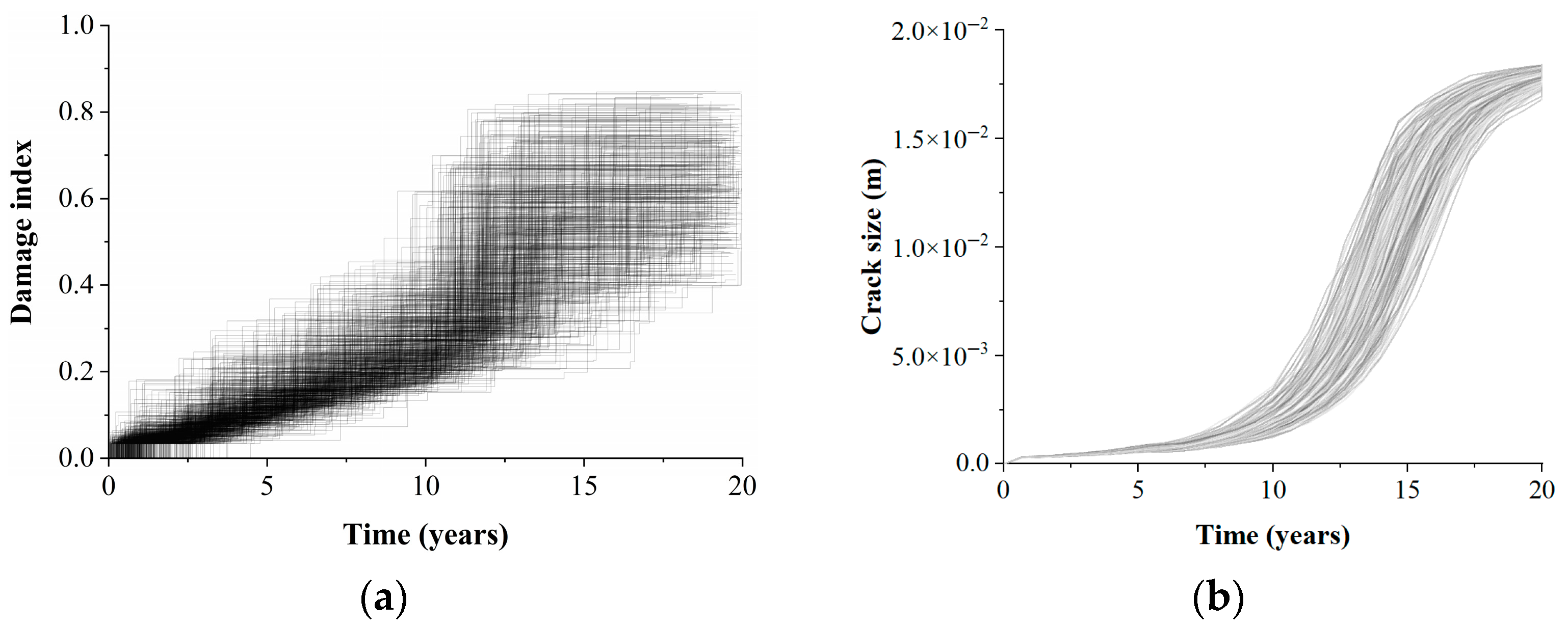
4.2. Fatigue Assessment

Fatigue is one of the principal phenomena that causes undesirable behavior in marine structures because it produces cracks at different hot spots of each joint. It is important to mention that each joint contributes differently to the overall capacity. For example, joints located in the lower part of the system usually contribute more, while joints located in the upper part of the system contribute less. It is possible to perform fatigue analysis for all joints; however, the contribution of some of them is negligible. Based on the above, it is assumed that fatigue analysis is carried out on those joints that contribute significantly to the overall capacity (critical joints). Critical joints are selected based on their contribution to the global capacity. The contribution is determined reducing the capacity of each joint; then, the global capacity is estimated by nonlinear static analysis. According to the above, the critical joints that provide the greatest capacity to the system are nodes 1 to 8. Two hot spots are defined for each end of the tubular element connected to the critical joints. The zone of hot spots presents both the maximum and the minimum stresses of each structural element. Several nonlinear dynamic step-by-step analyses are performed in the system to calculate the stresses of each hot spot using several simulated wave events related to different return periods. On the other hand, it is assumed that sea conditions have reached a fully developed state, which implies that wind has blown for a long period over a considerable distance, which leads to an equilibrium sea state. The spectra commonly used to describe fully developed sea states are the Jonswap [42], Pierson-Moskowitz [43], and Bretschneider [44]. In the absence of robust wave height data in the Campeche Bay, some authors have used the Pierson-Moskowitz spectrum to describe the frequency content of the waves with reasonable results [45,46,47]. Thus, the Pierson-Moskowitz [43] spectrum is used to describe the wave frequency content. It is assumed that a homogeneous Gaussian stationary process can be followed to describe the sea surface elevation as a superposition of regular waves considering phase angles between 0 and 2π. Monte Carlo simulation is employed to calculate the crack size at each hot spot using Equation (12). A set of thirty thousand simulations for crack growth in which the statistical moments become stable were considered. It is considered that the arrival times between storms are exponentially distributed [48].

Table 2. Statistical parameters utilized for simulating crack growth [49].

Parameter	Mean	Standard Deviation	Distribution
$a\left(t\right)$	According to the joint and time	According to the joint and time	Lognormal
$S_{mr}$	According to the joint and time	According to the joint and time	Rayleigh
$a/c$	0.25	-	-
M *	3	0.3	Normal
InC *	−40.39	−0.69067	Normal
$a_0$	0.00011	-	-

* Correlation coefficient = 0.9.

shows the statistical parameters obtained from offshore systems situated in the Gulf of Mexico.

The distribution functions related to both crack growth and mean stress interval are verified by means of the probability paper technique. Ref. [49] suggest that such distributions depend on both the joint and the time. Figure 4a shows the probability plot of the mean stress interval, $S_{mr}$, at one end of element 1, in which the continuous line represents the Rayleigh distribution function. Figure 4b shows the probability plot of the crack size, $a\left(t\right)$, at a hot spot of joint 1 for the time instant equal to 12 years. The continuous line expresses the lognormal distribution function. It is noticed that data of both stress interval and crack size acceptably fit their respective distribution function suggested in [49]. If the distribution functions used to characterize the crack size and mean stress interval are not suitable, a bias in the estimation of the cost of inspection and repair can be estimated.

Crack size at joints affects both the strength and the stiffness of the system. [50,51] suggest reducing the original capacity of joints using a linear reduction factor. Then, the reduced capacity of the cracked joint, $P_c$, is estimated as [50]:

$$P_c=P_k\left(1-{\frac{A_c}{A}}_j\right)$$

(15)

where $P_k$ is the intact joint capacity; $A_c$ is the cracking area of all elements connected to each joint, and $A_j$ corresponds to the intact joint area. Figure 5 shows the percentage of capacity reduction of the critical joint 1 for a set of thirty thousand simulations in a continuous gray line, while a continuous black line indicates the mean value of the reduction. It is observed that the joint capacity reduction due to fatigue is about 41.97% after 20 years of the offshore jacket installation.

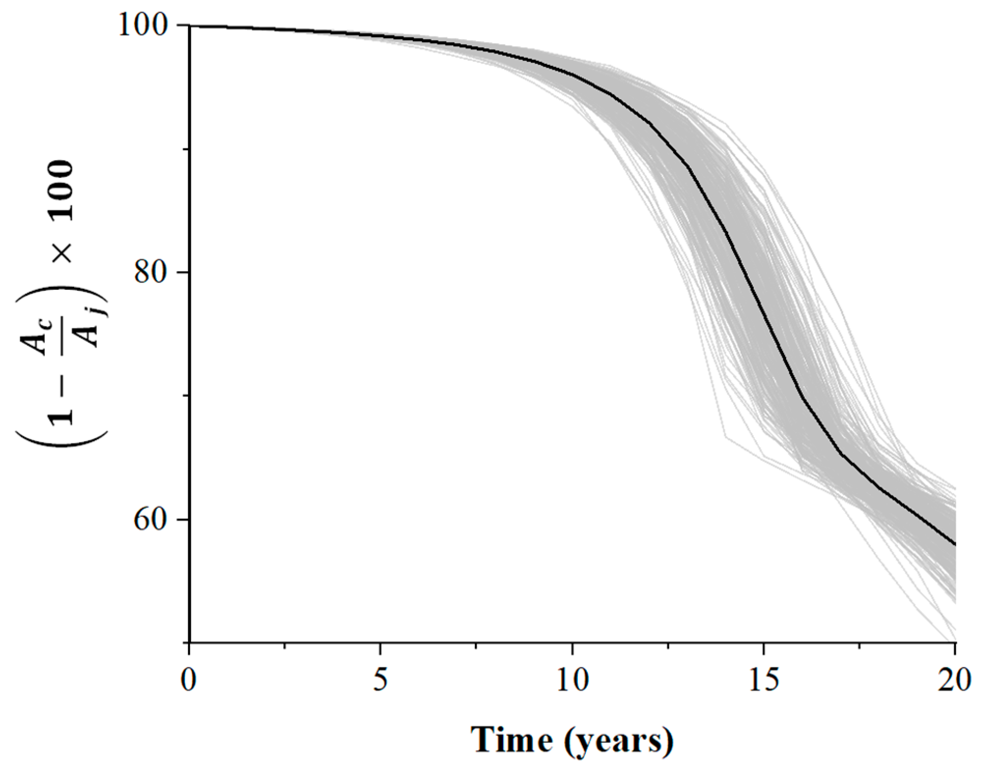
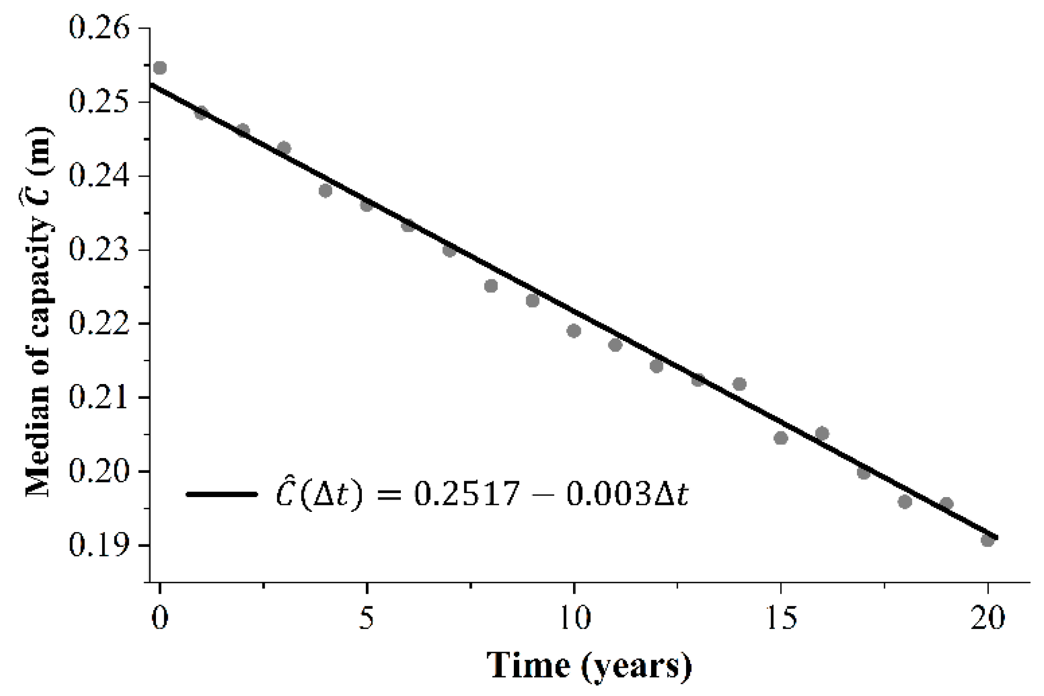
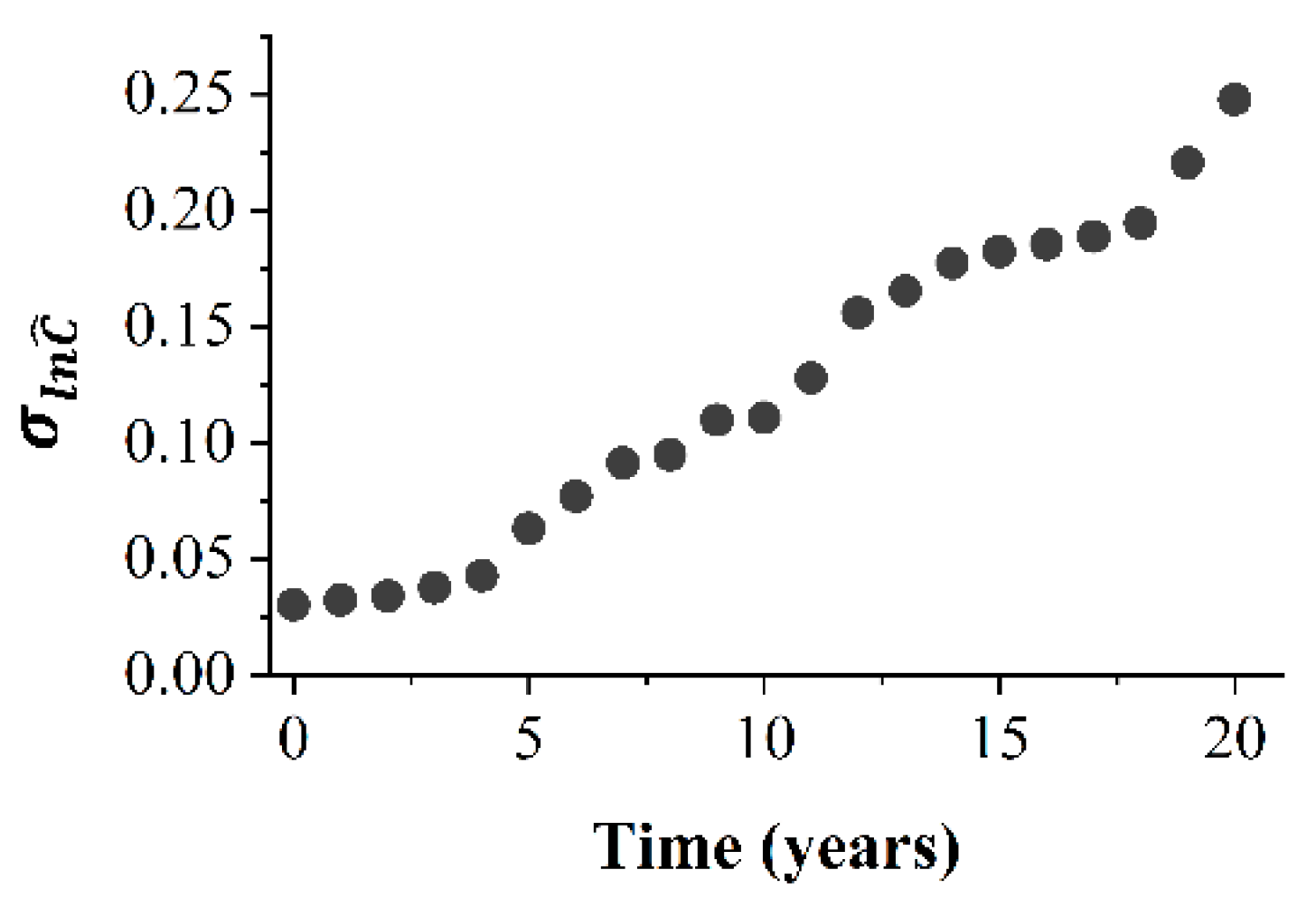
4.3. Structural Capacity

The structural capacity is obtained through non-linear static analysis employing a set of twenty lateral load profiles related to the return period of 1431 years [41]. The deterioration of the structure is given by the capacity reduction at each critical joint due to crack size from fatigue estimation. The median value of the global capacity due to cumulative damage caused by fatigue is shown in Figure 6. It is considered that the structural capacity follows a lognormal distribution function [28,30]. The global displacement at the deck is selected as indicator of the structural capacity. It is noticed that time instant $∆t$ = 0 represents the no damage condition of the system. The median values of the capacity show a reduction between 0.254 and 0.19 m for a period of 0 to 20 years, which indicates a decrease of 25.19% after 20 years after the system installation. Figure 6 shows the importance of considering the effect of the accumulated damage because the reliability of a certain system is commonly overestimated by assuming that the capacity remains constant over time. The median value of capacity is fitted by $\widehat{C}\left(∆t\right)={\alpha }_T-{\beta }_T∆t$. Figure 7 shows the standard deviation of the structural capacity over time. The values of the standard deviation are equal to 0.0302 at 0 years and 0.2478 at 20 years, indicating an increase of 820.52%, which is expected because the system is exposed to a greater number of storms and operational waves as time increases.

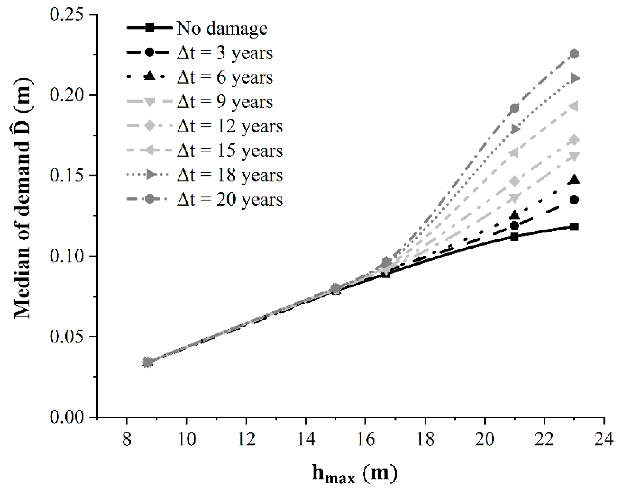
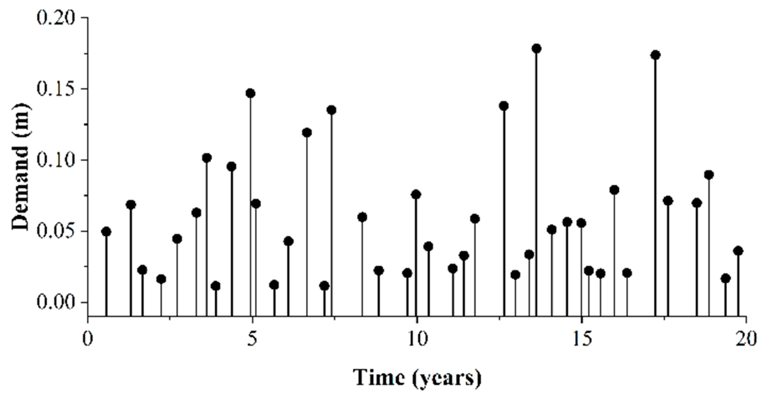
4.4. Structural Demand

The structural demand is calculated by employing nonlinear dynamic analyses using 20 simulations of waves related to different wave heights. With the purpose of considering the identical state of deterioration of the system to evaluate both capacity and demand at a given instant of time, it is feasible to use the capacity reductions obtained in Section 4.2, in which the capacity of each critical joint is reduced due to fatigue. The median value of structural demand, $\widehat{D}$, given a maximum wave height, $h_{max}$, at the time instant, $∆t$, is expressed by $\widehat{D}\left(∆t\right)=\left(a+f∆t\right)h_{max}^b$; the median values are fitted as $\widehat{D}\left(∆t\right)=\left(6.10\times {10}^{-6}+3.00\times {10}^{-7}∆t\right)h_{max}^{3.1}$. The standard deviation of the demand for a maximum wave height is expressed as ${\sigma }_{lnD│h_{max}}=\left(2.10\times {10}^{-3}+2.80\times {10}^{-5}∆t\right)h_{\mathrm{m}\mathrm{a}\mathrm{x}}^{1.4}$. Figure 8 shows the median values of the structural demand related to different wave heights. It is observed that the demand values for wave heights less than 15 m are similar, demonstrating that the system response is in its linear range. The median value of demand for instants 0, 3, 6, 9, 12, 15, 18 and 20 years at $h_{max}=23$ m are equal to 0.118, 0.134, 0.147, 0.162, 0.172, 0.193, 0.21 and 0.225 m, respectively. The above values indicate that the structural demand considering the cumulative damage due to fatigue, presents increments of 13.98%, 24.31%, 18.89%, 37.17%, 45.54%, 63.15%, 77.77% and 90.63% with respect to intact conditions ($∆t=0$). The above indicates that it is not suggested to omit structural deterioration because reliability considering demand without deterioration is different from reliability considering demand in an instant of time. Therefore, both the inspection and maintenance times of the system result longer, which leads to wrong decisions.

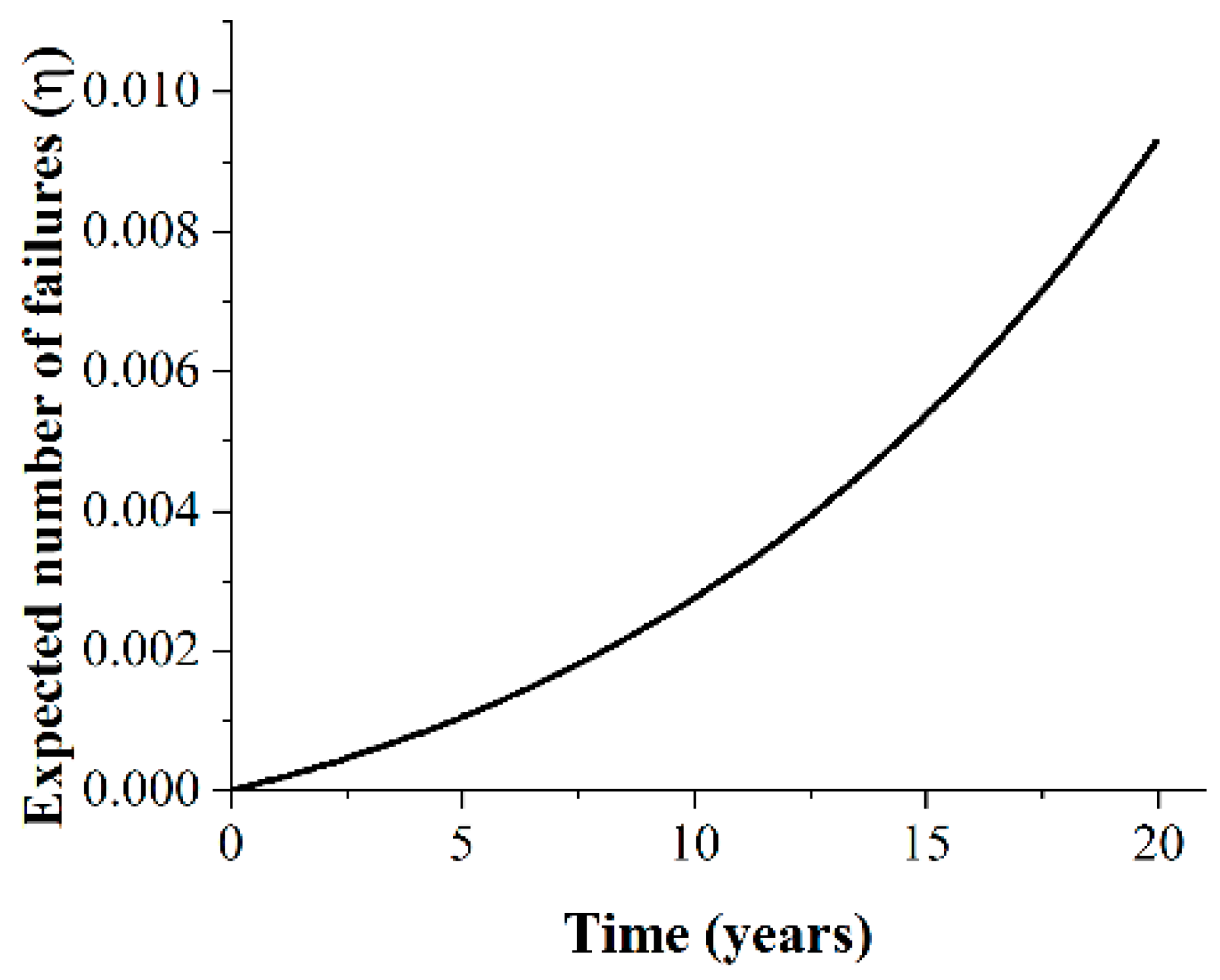
4.5. Expected Number of Failures

The expected number of failures, $\eta (0,∆t)$, are calculated using the statistical values of structural capacity and demand obtained in Section 4.3 and Section 4.4. The parameters $k$ and $r$ at $h_{max}=23$ m are equal to $5.8\times {10}^3$ and $5.2$. The epistemic uncertainties related to demand and capacity are equal to 0.15 [21]. Figure 9 shows the expected number of failures over time indicating an increase up to a value of 0.0093 at $∆t=20$ years. The expected number of failures associated to operational behavior (10 years) [41] is equal to 0.0027, which represents an increment of 1507.8% with respect to the time $∆t=1$ year. Notable differences are observed between 10 and 20 years, with an increase of 359.63%, which is attributed to years of operational wave action and storm events that accelerate fatigue damage, affecting the capacity of each critical joint.

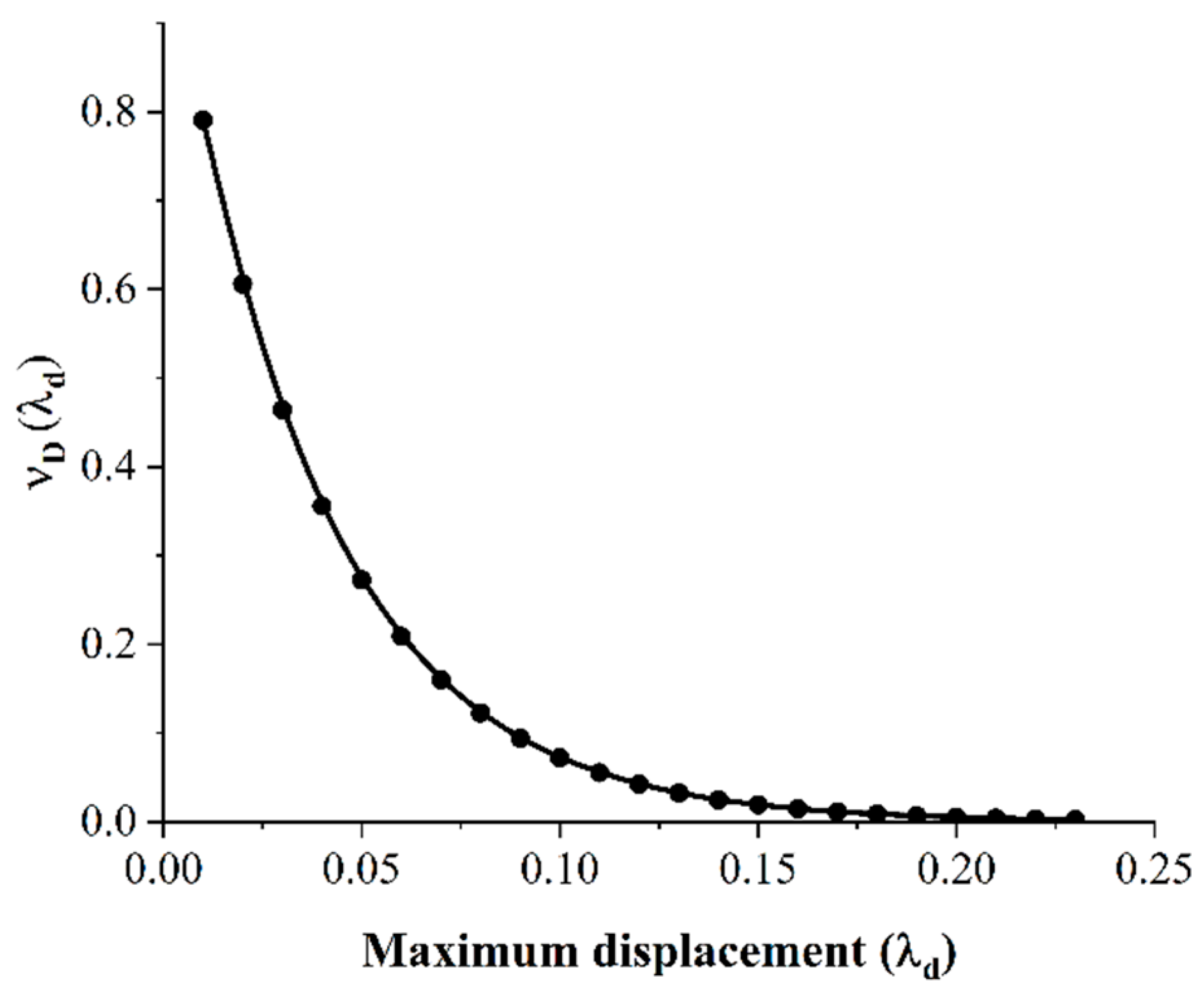
4.6. Demand Exceedance Rates

The demand exceedance rate expresses the number of times that a demand threshold of interest is exceeded per year, and its inverse indicates the return period of the demand threshold. The numerical exceedance demand rate is calculated using Equation (16) with both the information of Section 4.4 and the wave hazard of Section 4.1. Figure 10 shows different demand exceedance rates in terms of global displacement considering demand thresholds, ${\lambda }_d$, with values of 0.01, 0.02 up to 0.23 m. Figure 10 shows that the operational condition with a value of $h_{max}$ equal to 8.7 m [41] is associated with a threshold value of ${\widehat{D}=\lambda }_d=0.034$ (see Figure 8), which presents an exceedance rate equal to 0.4661. The above implies that the structure could exceed the operational condition 2.15 years after the system is built. Similar to the operational condition, the maximum wave height associated to the design condition, $h_{max}=16.7 \mathrm{m}$, is equal to 0.08 m. Based on the above, the return period of design condition is expected to be exceeded after 8.158 years. The ultimate resistance condition is associated to $h_{max}=23\mathrm{m}$ [41] and a value of ${\lambda }_d$ equal to 0.124 m at $∆t=0$ years, representing an exceedance rate equal to 0.0248 with a return period of being exceeded of 40.32 years.

Numerical demand exceedance rates can be fitted by the following expression [52]:

$${{\upsilon }_D\left(d\right)=\left(\frac{{\lambda }_d}{{{\lambda }_d}_0}\right)}^{-\xi }{\left(\frac{{{\lambda }_d}_{max}-{\lambda }_d}{{{\lambda }_d}_{max}-{{\lambda }_d}_0}\right)}^{\epsilon }$$

(16)

where ${{\lambda }_d}_0$ represents the calculated minimum demand value; ${{\lambda }_d}_{max}$ corresponds to the maximum demand value estimated; $\xi$ and $\epsilon$ are parameters that fit the shape of ${\upsilon }_D\left(d\right)$. The inverse transformation method [53], is used to simulate demand values; then, the cumulative distribution function of ${\upsilon }_D\left(d\right)$ is equal to $F\left(y\right)=1-{\upsilon }_D\left(d\right)/v_0$, $v_0$ represents the exceedance rate associated with the ${\lambda }_d$ considered. In this case, ${\lambda }_d$ equal to 0.01 corresponds to $v_0=0.8$. On the other hand, it is assumed that the arrival of demands can be described by a Poisson process; then, the waiting times of demands follow an exponential distribution [54]. After some mathematical arrangements, the demand occurrence time is $T_i=-\left|\mathit{ln}\left(u\right)/v_0\right|$; where $u$ represents random numbers [55]. Based on the above, two thousand realizations of demand and waiting times are simulated. Figure 11 shows only one realization.

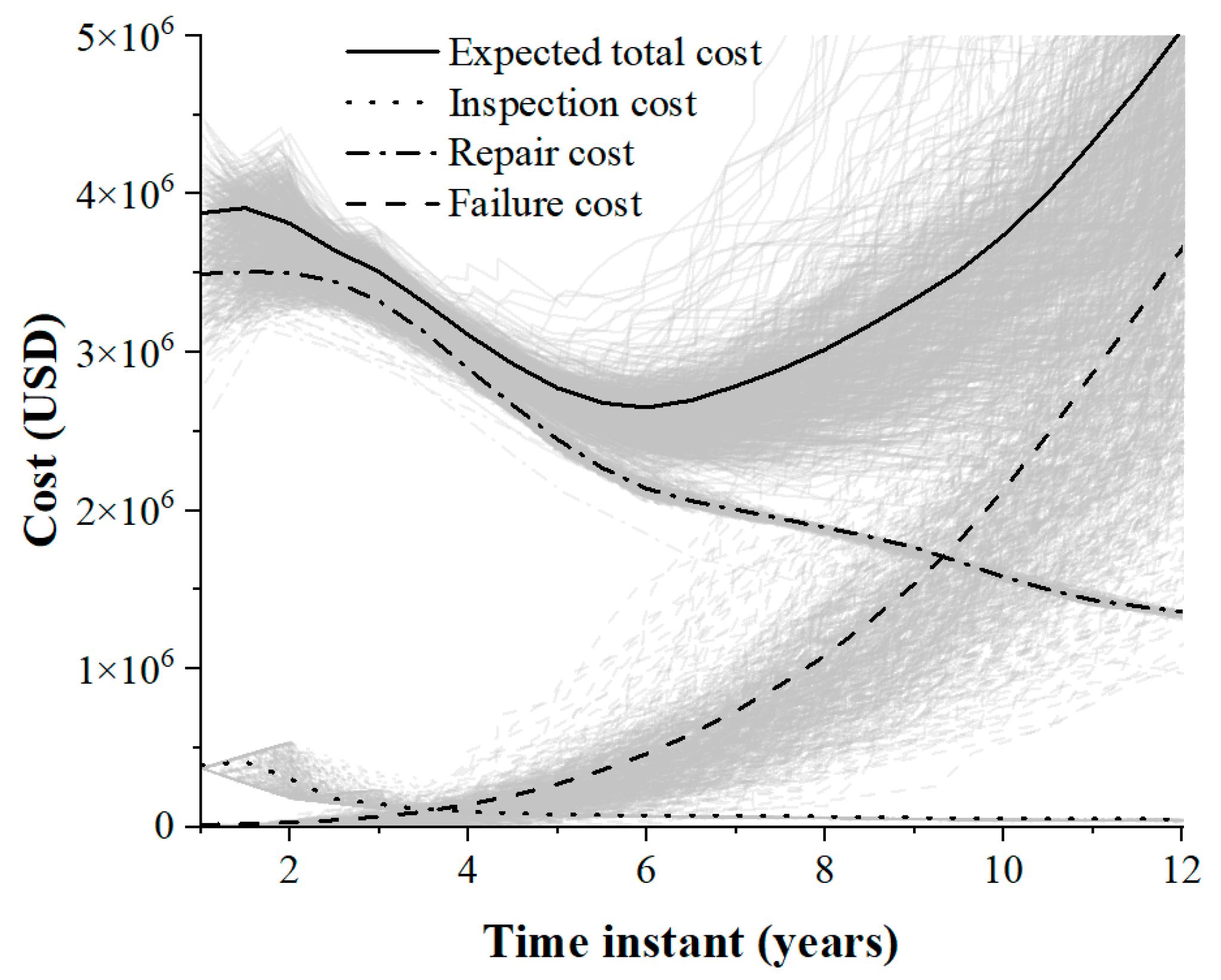
4.7. Optimal Time Instant

The optimal time instant for maintenance works is estimated by means of two thousand realizations of both demand and waiting times. The inspection, repair and failure costs are estimated per each simulated demand, whose arrival time matches the corresponding damage due to fatigue obtained in Section 4.2. The inspection cost is assumed in case that the probability of detecting a crack size of 2 mm [23] represents a secure event. If the crack size is detectable, the inspection cost per joint is equal to 3518 USD [56]. The visual inspection with divers is considered. Divers descend to perform the visual inspection using flashlights. The joint to be examined is recorded and photographed. Once the inspection is completed, the divers analyze their notes, photos, and recordings to give an opinion. The repair cost is applied at the time in which the conditional probability of the crack size exceeds the threshold of 4 mm [57]. This study considers that repair action is by welding with divers, and the cost of each hot spot equal to 20,000 USD [58]. Submarine welding with divers is usually performed as follows: (a) the surface joint is cleaned, and any coating or dirt is removed, (b) the area is sealed with bags or waterproof coatings, along with submersible blankets or covers, and (c) anti-corrosion weld is applied with special electrodes; either arc or pulsed welding technique can be used. If inspection and repair of the joints is not performed properly, the reliability of the system is affected. The inspection affects to a lesser degree because if no visible cracks are reported, the damage is accumulated up to the next inspection. However, if the joint repair has not been performed correctly, the assumption that the joint recovers its initial capacity is not satisfied. Then, the reliability of the system decreases, and undesired behavior could occur before the next inspection and maintenance work. The failure cost, $C_{F_m│ID,∆t}$, considers costs related to indirect losses, deferred production, and equipment damage. The cost related to indirect losses considers the consequences of the system presenting structural damage, impacting directly on other sectors such as power, agriculture, minerals, gas, basic chemicals, textile, tires and petrochemicals, among others, as follows:

$$C_{PID}=C_{F_T}\left(\frac{P_m}{P_t}\right){DI}^4$$

(17)

where $C_{F_T}$ is the cost of a loss related to the damaged system with a value equal to $1.086\times {10}^{10} \mathrm{U}\mathrm{S}\mathrm{D}$; $P_m$ is the production of oil barrels per day, equal to 184,000 [41], and $P_t$ corresponds to the total oil extracted per day in the Bay of Campeche with a value equal to 2,100,000 barrels [41].

The cost of pollution considers the volume of the oil spill over sea due to structural damage of the system as follows:

$$C_{POD}=\frac{C_{OR}·S_A·E_f}{\mathrm{1,000,000}}$$

(18)

where $C_{OR}$ is the cost of oil recovery, equal to 541.57 USD per hour considering an efficiency, $E_f$, of $0.81\mathrm{h}/\mathrm{k}{\mathrm{m}}^2$ [59], and $S_A$ represents the affected area [59] as follows:

$$S_A=0.04∆w{P}_{m}D{I}^4{U}^4+2.27{\left(∆w{P}_{m}D{I}^4\right)}^{\frac{2}{3}}{t}^{\frac{1}{2}}$$

(19)

where $∆w$ is the difference of densities between water and oil equal to $0.06341$; $t$ represents the time of oil spill with a value of $2400 \mathrm{s}$ and $U$ is equal to $30 \mathrm{m}/\mathrm{s}$.

Deferred production cost is estimated as follows [60]:

$$C_{DPC}=365{\int }_t^{DL}{C}_C{P}_m{U}_C\exp \left[-{\gamma }_m\left(\tau -t\right)\right]d\tau -365{\int }_t^{DL+T_{RP}}{C}_C{P}_m{U}_C\exp \left[-{\gamma }_m\left(\tau -t\right)\right]d\tau$$

(20)

where $DL$ is equal to 30 years [28]; $C_C$ is the price of crude oil, equal to 92 $\mathrm{U}\mathrm{S}\mathrm{D}/\mathrm{b}\mathrm{a}\mathrm{r}\mathrm{r}\mathrm{e}\mathrm{l}$; $U_C$ represents the economic benefit of selling, equal to $12\mathrm{\%}$; $T_{RP}$ is the time to recover the product, with a value of four years. The annual discount rate, ${\gamma }_m$, is equal to 6% [21].

The equipment damage cost relates the structural damage in terms of $DI$ to the cost of equipment as follows:

$$C_{EQD}=DI·C_{EQPT}$$

(21)

where $C_{EQPT}$ is the cost of the drilling equipment, with a value of 130,000,000 USD [61].

Equation (1) can be evaluated using expected or simulated values. The variables that influence the simulation of the expected total cost are crack size, demand and capacity on the system. Crack size is involved in (a) the inspection quality, $q$, for the inspection cost and (b) the probability that a certain crack size in the $j-th$ element at ∆t exceeds a given threshold, $P\left(D_{j,m}\left(∆t\right)\ge d\right)$, in case of repair cost. Demand and capacity modify the expected number of failures, ${\overline{\eta }}_F\left(0,∆t\right)$, that are found in the cost of inspection, repair, and failure. The lognormal probability distribution function is used to simulate the crack size, $a\left(t\right)$, and the statistical parameters of crack size depend on the joint and the time instant of interest, as shown in Table 2. Structural demand is simulated based on the considerations described in Section 4.6, in which demand and waiting times are simulated (see Figure 11). Based on the arrival time of each demand, the capacity is simulated with the help of the statistical values shown in Figure 6 and Figure 7. The damage index, $DI$, is calculated over time using the simulated values of demand and capacity. Figure 12a,b show the damage index and an example of crack size at one hot spot of joint 1 over time for two thousand simulations.

Using Equation (1) and the procedure described in Section 3, Figure 13 shows the inspection, repair, failure, and expected total cost. Each cost of the inspection is shown with a gray dotted line, the repair cost in a dashed and dotted gray line, the failure cost in a dashed gray line, and the expected total cost in a continuous gray line. The mean values of each cost are shown with the same type of line in black color. Figure 13 shows that inspection and repair costs present a greater dispersion for shorter periods, while the failure cost shows dispersion in greater time intervals. Such behaviors are due to the following: (1) for intervals between 1 and 3 years, the inspection quality influences the decision of whether to perform inspection actions or not, due to the probability of detecting a certain value of crack size; (2) for periods of time smaller than four years, the crack size defines the conditional probability related to maintenance; after four years of time interval, the conditional probability tends to be an event with a certain probability value; then, the repair costs are activated until they result in certain to occur event, in which the cost of repairing all critical joints becomes constant as time increases; (3) the failure cost presents low dispersion values due to both time intervals less than 6 years with low probability that a high value of demand occurs and low values of the expected number of failures, $\eta \left(0,∆t\right).$ Nevertheless, as the time interval increases, both $\eta (0,∆t)$ and the probability of occurrence of a high demand value increase, resulting in different failure cost values. Moreover, a reduction of inspection and repair costs is observed as the instant of time increases, while the failure costs increase with longer time instants. The minimum mean value of the expected total cost (continuous black line) results in a value of 6 years, indicating the optimal time instant for maintenance works in the system.

Table 3. Expected mean costs at different time instants.

Time Instant (Years)	Inspection Cost $\times {10}^6 \mathbf{U}\mathbf{S}\mathbf{D}$	Repair Cost $\times {10}^6 \mathbf{U}\mathbf{S}\mathbf{D}$	Failure Cost $\times {10}^6 \mathbf{U}\mathbf{S}\mathbf{D}$	Expected Total Cost $\times {10}^6 \mathbf{U}\mathbf{S}\mathbf{D}$
1	0.38	3.48	0.00	3.87
3	0.13	3.31	0.05	3.50
6	0.06	2.13	0.45	2.64
9	0.05	1.75	1.52	3.32
12	0.04	1.35	3.64	5.03

shows the expected mean values of inspection, repair, failure, and total cost at different time instants. It is observed that the cost of inspection and repair increase for short time instants due to higher number of interventions that are necessary during the lifetime of the system. The cost of failure is not influenced by short time instants because the expected number of failures results in a low value. However, as the time interval increases, the value of the expected number of failures increases, which directly affects the cost of failure. In the literature, there are proposals for maintenance plans in which the optimal time instant is estimated in 18 years [62], 10 years [63] and 5 years [64]. Although the proposed approaches consider different assumptions and the systems are located at different sites, the time instants for inspection and maintenance actions are consistent with the time instant found in this work.

5. Conclusions

A probabilistic approach to calculate the optimal time instant for maintenance works considering the structural damage due to fatigue over time was proposed. The optimal time instant is estimated in accordance with a CB, in which different costs, such as inspection, repair, and failure, are considered. The system reliability is defined in terms of the expected number of failures. The approach can be applied to any type of offshore system and can be changed for its use in other structural systems under different environmental conditions.

The approach is illustrated with an offshore jacket structure. The calculated cost of failure without inspection and maintenance actions in 30 years is equal to 31.74 × 10⁶ USD. If inspection and maintenance actions are performed at the optimal time instant of 6 years, five interventions in 30 years are required, with a total cost of 13.20 × 10⁶ USD, which represents a reduction of 58.4%, compared to the cited failure cost. The optimal time instant is related to an expected number of failures equal to 0.0014, while at $∆t=20$ years the value is 0.0093, which represents an increase of 84.94%. The exceedance demand rate associated with the operational condition (8.7 m of wave height) is equal to 0.034, and its inverse indicates that such condition is expected to be exceeded 29.41 years after the jacket installation, which suggests that the optimal time instant is appropriate, and does not compromise the performance of the system. The above is valid for similar system topology, wave loads, and sites.

The approach helps decision-making and risk management to maintain the system at acceptable reliability levels and minimum costs, which help to extend the lifespan of the system. On the other hand, the approach requires solving a hypergeometric function, which makes it impractical for structural engineers, and requires considerable computational time to obtain the optimal time instant. The approach can be improved to consider multiple offshore platforms to find a common minimum cost, which would help to reduce costs at the offshore oil complex. The proposed approach can be compared with other techniques such as multiobjective optimization to identify areas for improvement. In addition, climate change can be included in the optimization problem to improve the characterization of the physical problem. The above represents a challenge because it requires several studies on the increase of sea level, and occurrences and intensity of hurricanes, among other aspects that affect the performance of the system. Then, maintenance time instants could be reduced.

References

1. Zou, C.; Zhao, Q.; Zhang, G.; Xiong, B. Energy revolution: From a fossil energy era to a new energy era. Nat. Gas Ind. B 2016, 3, 1–11. [Google Scholar] [CrossRef] [Green Version]
2. SENER. Prospectiva de Petróleo Crudo y Petrolíferos 2016–2030; Secretaría de Energía: Mexico City, Mexico, 2016. [Google Scholar]
3. Herrera, D.; Varela, G.; Tolentino, D. Reliability Assessment of RC Bridges Subjected to Seismic Loadings. Appl. Sci. 2021, 12, 206. [Google Scholar] [CrossRef]
4. Mohammed, D.; Al-Zaidee, S. Deflection Reliability Analysis for Composite Steel Bridges. Eng. Technol. Appl. Sci. Res. 2022, 12, 9155–9159. [Google Scholar] [CrossRef]
5. Fanaie, N.; Kolbadi, M.S. Probabilistic seismic demand assessment of steel moment-resisting frames with mass irregularity in height. Sci. Iran. 2019, 26, 1156–1168. [Google Scholar] [CrossRef] [Green Version]
6. Gavabar, S.G.; Alembagheri, M. Structural demand hazard analysis of jointed gravity dam in view of earthquake uncertainty. KSCE J. Civ. Eng. 2018, 22, 3972–3979. [Google Scholar] [CrossRef]
7. El-Din, M.N.; Kim, J. Simplified seismic life cycle cost estimation of a steel jacket offshore platform structure. Struct. Infrastruct. Eng. 2017, 13, 1027–1044. [Google Scholar] [CrossRef]
8. Zekavati, A.A.; Jafari, M.A.; Mahmoudi, A. Regional Multihazard Risk-Assessment Method for Overhead Transmission Line Structures Based on Failure Rate and a Bayesian Updating Scheme. J. Perform. Constr. Facil. 2022, 37, 04022068. [Google Scholar] [CrossRef]
9. Praxedes, C.; Yuan, X.X. Robustness-oriented optimal design for reinforced concrete frames considering the large uncertainty of progressive collapse threats. Struct. Saf. 2022, 94, 102139. [Google Scholar] [CrossRef]
10. Khajehzadeh, M.; Kalhor, A.; Tehrani, M.S.; Jebeli, M. Optimum design of retaining structures under seismic loading using adaptive sperm swarm optimization. Struct. Eng. Mech. 2022, 81, 93–102. [Google Scholar] [CrossRef]
11. Mai, H.T.; Lee, S.; Kim, D.; Lee, J.; Kang, J.; Lee, J. Optimum design of nonlinear structures via deep neural network-based parameterization framework. Eur. J. Mech.-A/Solids 2023, 98, 104869. [Google Scholar] [CrossRef]
12. Fan, Z.; Ye, Q.; Xu, X.; Ren, Y.; Huang, Q.; Li, W. Fatigue reliability-based replacement strategy for bridge stay cables: A case study in China. Structures 2022, 39, 1176–1188. [Google Scholar] [CrossRef]
13. Abdelkader, E.M.; Moselhi, O.; Marzouk, M.; Zayed, T. An exponential chaotic differential evolution algorithm for optimizing bridge maintenance plans. Autom. Constr. 2022, 134, 104107. [Google Scholar] [CrossRef]
14. Chadha, M.; Ramancha, M.K.; Vega, M.A.; Conte, J.P.; Todd, M.D. The modeling of risk perception in the use of structural health monitoring information for optimal maintenance decisions. Reliab. Eng. Syst. Saf. 2023, 229, 108845. [Google Scholar] [CrossRef]
15. Vrijdaghs, R.; Verstrynge, E. Probabilistic structural analysis of a real-life corroding concrete bridge girder incorporating stochastic material and damage variables in a finite element approach. Eng. Struct. 2022, 254, 113831. [Google Scholar] [CrossRef]
16. Ontiveros-Pérez, S.P.; Miguel, L.F.F. Reliability-based optimum design of multiple tuned mass dampers for minimization of the probability of failure of buildings under earthquakes. Structures 2022, 42, 144–159. [Google Scholar] [CrossRef]
17. Cheng, J.; Jin, H. Reliability-based optimization of steel truss arch bridges. Int. J. Steel Struct. 2017, 17, 1415–1425. [Google Scholar] [CrossRef]
18. Zou, G.; Faber, M.H.; González, A.; Banisoleiman, K. Fatigue inspection and maintenance optimization: A comparison of information value, life cycle cost and reliability based approaches. Ocean Eng. 2021, 220, 108286. [Google Scholar] [CrossRef]
19. Lotsberg, I.; Sigurdsson, G.; Fjeldstad, A.; Moan, T. Probabilistic methods for planning of inspection for fatigue cracks in offshore structures. Mar. Struct. 2016, 46, 167–192. [Google Scholar] [CrossRef]
20. Dyer, A.S.; Zaengle, D.; Nelson, J.R.; Duran, R.; Wenzlick, M.; Wingo, P.C.; Bauer, J.R.; Rose, K.; Romeo, L. Applied machine learning model comparison: Predicting offshore platform integrity with gradient boosting algorithms and neural networks. Mar. Struct. 2022, 83, 103152. [Google Scholar] [CrossRef]
21. Tolentino, D.; Ruiz, S.E. Time Intervals for Maintenance of Offshore Structures Based on Multiobjective Optimization. Math. Probl. Eng. 2013, 2013, 125856. [Google Scholar] [CrossRef] [Green Version]
22. Wang, M.; Leng, J.; Feng, S.; Li, Z.; Incecik, A. Precisely modeling offshore jacket structures considering model parameters uncertainty using Bayesian updating. Ocean Eng. 2022, 258, 111410. [Google Scholar] [CrossRef]
23. Schoefs, F.; Tran, T.B. Reliability Updating of Offshore Structures Subjected to Marine Growth. Energies 2022, 15, 414. [Google Scholar] [CrossRef]
24. Heo, T.; Nguyen, P.T.T.; Manuel, L.; Collu, M.; Abhinav, K.A.; Xu, X.; Brizzi, G. Operations and Maintenance for Multipurpose Offshore Platforms using Statistical Weather Window Analysis. In Proceedings of the Global Oceans 2020: Singapore–US Gulf Coast, Biloxi, MS, USA, 5–30 October 2020. [Google Scholar] [CrossRef]
25. De León Escobedo, D.; Alfredo, H.S. Development of a cost-benefit model for the management of structural risk on oil facilities in Mexico. Comput. Struct. Eng. An. Int. J. 2002, 2, 19–23. [Google Scholar]
26. Ortega Estrada, C.E.; De León Escobedo, D. Development of a Cost-Benefit Model for Inspection of Offshore Jacket Structures in Mexico. In Proceedings of the Offshore Mechanics and Arctic Engineering, Cancun, Mexico, 8–13 June 2003. [Google Scholar] [CrossRef]
27. Santa-Cruz, S.; Heredia-Zavoni, E. Maintenance and decommissioning real options models for life-cycle cost-benefit analysis of offshore platforms. Struct. Infrastruct. Eng. 2009, 7, 733–745. [Google Scholar] [CrossRef]
28. Tolentino, D.; Ruiz, S.E. Influence of structural deterioration over time on the optimal time interval for inspection and maintenance of structures. Eng. Struct. 2014, 61, 22–30. [Google Scholar] [CrossRef]
29. Yoon, J.T.; Youn, B.D.; Yoo, M.; Kim, Y.; Kim, S. Life-cycle maintenance cost analysis framework considering time-dependent false and missed alarms for fault diagnosis. Reliab. Eng. Syst. Saf. 2019, 184, 181–192. [Google Scholar] [CrossRef]
30. Tolentino, D.; Ruiz, S.E.; Torres, M.A. Simplified closed-form expressions for the mean failure rate of structures considering structural deterioration. Struct. Infrastruct. Eng. 2012, 8, 483–496. [Google Scholar] [CrossRef]
31. Rainville, D. Intermediate Course in Differential Equations, 1st ed.; John Wiley and Sons, Inc.: Hoboken, NJ, USA, 1943. [Google Scholar]
32. Ritger, P.D.; Rose, N.J. Differential Equations with Applications, 1st ed.; Dover Publications: New York, NY, USA, 2000. [Google Scholar]
33. Visser, W. POD/POS Curves for Non-Destructive Examination, Offshore Technology Report OTO-2000/018; Health & Safety Executive: Weybridge, Surrey, UK, 2002. [Google Scholar]
34. Moan, T.; Hovde, G.O.; Blanker, A.M. Reliability-based fatigue criteria for offshore structures considering the effect of inspection and repair. In Proceedings of the Offshore Technology Conference, Houston, TX, USA, 3–6 May 1993; pp. 591–597. [Google Scholar] [CrossRef]
35. Rangel-Ramirez, J.G.; Sørensen, J.D. Optimal risk-based inspection planning for offshore wind turbines. Int. J. Steel Struct. 2008, 8, 295–303. [Google Scholar]
36. Moan, T. Reliability-based management of inspection, maintenance and repair of offshore structures. Struct. Infrastruct. Eng. 2007, 1, 33–62. [Google Scholar] [CrossRef]
37. Paris, P.; Erdogan, F. A Critical Analysis of Crack Propagation Laws. J. Basic Eng. 1963, 85, 528–533. [Google Scholar] [CrossRef]
38. Newman, J.C.; Raju, I.S. An empirical stress-intensity factor equation for the surface crack. Eng. Fract. Mech. 1981, 15, 185–192. [Google Scholar] [CrossRef]
39. Sobczyk, K.; Spencer, B.F., Jr. Random Fatigue: From Data to Theory, 1st ed.; Academic Press: Cambridge, MA, USA, 1992. [Google Scholar]
40. Cornell, C.A.; Jalayer, F.; Hamburger, R.O.; Foutch, D.A. Probabilistic Basis for 2000 SAC Federal Emergency Management Agency Steel Moment Frame Guidelines. J. Struct. Eng. 2002, 128, 526–533. [Google Scholar] [CrossRef] [Green Version]
41. PEMEX. Diseño y Evaluación de Plataformas Marinas Fijas en la Sonda de Campeche; Petroleos Mexicanos: Mexico City, Mexico, 2000. [Google Scholar]
42. Hasselmann, K.; Barnett, T.P.; Bouws, E.; Carlson, H.; Cartwright, D.E.; Enke, K.; Ewing, J.A. Measurements of wind-wave growth and swell decay during the joint North Sea wave project (JONSWAP). Ergaenzungsheft Zur Dtsch. Hydrogr. Z. Reihe A 1973, 8, 1–95. [Google Scholar]
43. Pierson, W.J.; Moskowitz, L. A proposed spectral form for fully developed wind seas based on the similarity theory of S. A. Kitaigorodskii. J. Geophys. Res. 1964, 69, 5181–5190. [Google Scholar] [CrossRef]
44. Bretschneider, C.L. Wave variability and wave spectra for wind-generated gravity waves. Beach Erosion Board. US Army Corps Eng. Tech. Memo 1959, 118, 1–192. [Google Scholar]
45. Torres, M.A.; Ruiz, S.E. Structural reliability evaluation considering capacity degradation over time. Eng. Struct. 2007, 29, 2183–2192. [Google Scholar] [CrossRef]
46. Silva-Ballesteros, J.; Barranco-Cicilia, F. Statistic Comparison between Wave Height Time Histories from Different Simulation Techniques for a Campeche Bay Sea State. In Proceedings of the Seventh International Offshore and Polar Engineering Conference, Honolulu, HI, USA, 25–30 May 1997. [Google Scholar]
47. De Leon, D. Reliability-Based Assessment of Vibrations on an Offshore Living-Quarters Platform in Mexico. In Proceedings of the Offshore Mechanics and Arctic Engineering, Oslo, Norway, 23–28 June 2002. [Google Scholar] [CrossRef]
48. Lee, S.; Wilson, J.R.; Crawford, M.M. Modeling and simulation of a nonhomogeneous poisson process having cyclic behavior. Commun. Stat.-Simul. Comput. 2007, 20, 777–809. [Google Scholar] [CrossRef]
49. Silva-González, F.L.; Heredia-Zavoni, E. Effect of Uncertainties on the Reliability of Fatigue Damaged Systems. In Proceedings of the Offshore Mechanics and Arctic Engineering, Vancouver, BC, Canada, 20–25 June 2004. [Google Scholar] [CrossRef]
50. Stacey, A.; Sharp, J.V.; Nichols, N.W. Static Strength Assessment of Cracked Tubular Joints; American Society of Mechanical Engineers: New York, NY, USA, 1996. [Google Scholar]
51. Burdekin, F.M. The Static Strength of Cracked Joints in Tubular Members, Offshore Technology Report OTO-2001/080; Health & Safety Executive: Weybridge, Surrey, UK, 2001. [Google Scholar]
52. Tolentino, D.; Flores, R.B.; Alamilla, J.L. Probabilistic assessment of structures considering the effect of cumulative damage under seismic sequences. Bull. Earthq. Eng. 2018, 16, 2119–2132. [Google Scholar] [CrossRef]
53. Vogel, C.R. Computational Methods for Inverse Problems; Society for Industrial and Applied Mathematics: Philadelphia, PA, USA, 2002. [Google Scholar]
54. Melchers, R.E.; Beck, A.T. Structural Reliability Analysis and Prediction; John Wiley & Sons Ltd.: Chichester, UK, 2017. [Google Scholar] [CrossRef]
55. Tolentino, D.; Márquez-Domínguez, S.; Gaxiola-Camacho, R. Fragility Assessment of Bridges Considering Cumulative Damage Caused by Seismic Loading. KSCE J. Civ. Eng. 2020, 24, 551–560. [Google Scholar] [CrossRef]
56. Raine, A. The development of alternating current field measurement (ACFM) technology as a technique for the detection of surface breaking defects in conducting material and its use in commercial and industrial applications. In Proceedings of the 15th World Conference on Non-Destructive Testing, Rome, Italy, 15–21 October 2000. [Google Scholar]
57. Kirkemo, F. Applications of probabilistic fracture mechanics to offshore structures. Appl. Mech. Rev. 1988, 41, 61–84. [Google Scholar] [CrossRef]
58. Jardine, R.J.; Chow, F.C. New Design Methods for Offshore Piles; MTD Ltd. Publication; Marine Technology Directorate: Tipton, UK, 1996. [Google Scholar]
59. Campos, D.; Rodriguez, M.; Martinez, M.; Ramos, R. Assessment of consequences of failure in jacket structures. In Proceedings of the Offshore Mechanics and Arctic Engineering, St. John’s, NL, Canada, 11–16 July 1999. [Google Scholar]
60. McClelland, B.; Reifel, M.D. Planning and Design of Fixed Offshore Platforms, 1st ed.; Springer Publishing: New York, NY, USA, 1986. [Google Scholar]
61. IMP. Resumen Ejecutivo de Costos Promedio de Estructuras Típicas Ubicadas en la Sonda de Campeche; Instituto Mexicano del Petroleo: Mexico City, Mexico, 1998. [Google Scholar]
62. Faber, M.H.; Kroon, I.B.; Sørensen, J.D. Sensitivities in structural maintenance planning. Reliab. Eng. Syst. Saf. 1996, 51, 317–329. [Google Scholar] [CrossRef]
63. Straub, D.; Faber, M.H. Risk based inspection planning for structural systems. Struct. Saf. 2005, 27, 335–355. [Google Scholar] [CrossRef]
64. Goyet, J.; Straub, D.; Faber, M.H. Risk based inspection planning. Methodol. Appl. Offshore Struct. 2011, 6, 489–503. [Google Scholar] [CrossRef]
Figure 1. Drilling platform (a) profile view and (b) joint damage.
Jmse 11 01348 g001
Figure 2. Offshore fixed platform.
Jmse 11 01348 g002
Figure 3. Environmental hazard: (a) Maximum wave, (b) wind speed and (c) sea currents.
Jmse 11 01348 g003
Figure 4. Probability plot: (a) mean stress interval; (b) crack size.
Jmse 11 01348 g004
Figure 5. Reduction areas at joint 1.
Jmse 11 01348 g005
Figure 6. Median of the structural capacity.
Jmse 11 01348 g006
Figure 7. Standard deviation of the natural logarithm of capacity.
Jmse 11 01348 g007
Figure 8. Median of the structural demand.
Jmse 11 01348 g008
Figure 9. Expected number of failures.
Jmse 11 01348 g009
Figure 10. Numerical demand exceedance rates.
Jmse 11 01348 g010
Figure 11. Realization of demand and waiting times.
Jmse 11 01348 g011
Figure 12. (a) Damage index and (b) crack size simulation.
Jmse 11 01348 g012
Figure 13. Expected costs.
Jmse 11 01348 g013