Unified System Analysis for Time-Variant Reliability of a Floating Offshore Substation

Abstract

Offshore wind is planned to become the first source of energy by 2050. That requires installing turbines in deeper seas. It is shown that only floating wind turbines will allow dealing with this challenge while keeping a reasonable cost of energy production and transport according to the levelized cost of electricity. A Floating Offshore Substation will be needed in many sites. This technology is still at a low technology readiness level. This paper aims to analyze the system reliability of such a structure for which the failure rates of structural components such as mooring lines and dynamic power cables are close to the ones of electro-technical systems. Consequently, only a system reliability assessment of the floating offshore substation will allow accurately quantifying its availability and the most sensitive components. Usually, structural reliability aims at quantifying the probability of failures, while electro-technical reliability relies on feedback and observed failure rates. The paper first unifies these two concepts in a single formulation and then evaluates the system’s reliability and availability. This methodology is illustrated in a study case localized in the French coasts of the Mediterranean Sea, where the effect of several mooring and substation designs on the system reliability is compared.

1. Introduction

Offshore wind is planned to become the first source of energy by 2050 in view to meet the maximum levels of CO₂ emissions in the world [1]. In its report on “Future Wind”, the International Renewable Energy Agency predicts first a rapid growth in the offshore wind annual market to 2050 [2], with a rise of more than six-fold in 2030 and around ten-fold in 2050. To achieve this objective, it is necessary to examine unexplored locations where there is a valuable resource, but deep water poses a challenge in installing fixed structures, particularly in transitional (60 m or deeper) to large (300 m or deeper) water depths. In certain regions, such as the west coast of the USA and Mediterranean sites in France and Spain, the water depth can be significant even near the shoreline. In other areas, these water depths may be encountered further from the coast but are being considered for future development due to conflicts between usage and acceptability [3]. Such constraints force the farm operators, technology developers, Transmission System Operators (TSOs), and the whole Marine Renewable Energy (MRE) sector to consider new solutions for the implementation of Offshore Substations (OSSs). Floating foundation is the innovation that will have the highest impact in opening new markets and decreasing environmental impact [2].

The usual way to connect commercial fixed farms is to use regular topside design inspired by Oil and Gas offshore platforms and called (static) Offshore Substations. Floating offshore substations are key components due to their central role and their novelty—e.g., electrical material subjected to permanent inertial loads—bringing high expectations on the object. The specificity of the floating or sub-sea substation, as compared to a fixed substation, is therefore in the use of components deployed between the seabed and the floating wind or tidal and the floating substation. These mechanical or electrical elements are solicited by the movements of the floating support, the swell, and the marine current and are moreover sensitive to bio-fouling. This equipment, used in onshore wind farms or in offshore Oil and Gas, must be redesigned for an optimal fit to the actual marine renewable energy environment. They must be designed specifically to withstand the stresses of harsh environments during a period of 25 years. Internal components of the substation are therefore likely to be different from the ones used in conventional static substations.

More studies focus on floating offshore turbines but much less on the reliability of one of the most critical components in a wind farm: the offshore substation [4]. Oh et al. [5] present a review of the foundations of offshore wind energy substations. Different concepts of substructures are needed to lower construction costs for transitional water depth. Space frame substructures such as tripod and jacket structures can provide the required strength and stiffness. Tripod and jacket structures provide sufficient bearing capacity in transitional water depths with relatively short penetration lengths. Moreover, the relatively low weight of tripods and jackets enhances the economic feasibility. The Alpha Ventus and Beatrice demonstration projects encourage the development of offshore wind farms with this substructure in transitional water depth. A Floating Offshore Substation (FOSS) could be a relevant solution, provided that the dynamic cables are required to plug it from both the power generation and the grid sides. This brings the most significant design constraint as the voltage level will be significantly higher.

There is no specific lesson learned on design rules and life expectancy today for FOSSs regarding renewable energy production, even if some lower voltage installations exist in Oil and Gas. Today, and only one unit exists in Japan [6]. The actual knowledge relies mainly on two domains:

• Offshore wind turbine installed: the substations are fixed on the seabed. The difficulties are mainly in minimizing their footprint and comprehending the environmental impact on equipment.
• Offshore oil and gas in deep water (i.e., deeper than 1000 m) uses a floating production structure and flexible bottom-surface links. The R&D work carried out over the last 25 years in this area makes it possible to obtain results, calculation tools, and standards that are regularly updated. Unfortunately, they are specific to floating structures of very large dimensions (weak movements) and are little sensitive to swell and bio-fouling. Despite an important experience, offshore Oil and Gas continues R&D work continuously to optimize sizing methods, standards, and therefore safety factors.

Compared to a fixed substation, an FOSS is unique in its use of components that are deployed between the seabed and the floating wind or tidal device, as well as the floating substation. These mechanical or electrical elements are subjected to the movements of the floating support, the swell, and the marine current, as well as bio-fouling, making them sensitive. These components must be redesigned for an optimal fit with actual marine renewable energies, as they are used in onshore wind farms or offshore Oil and Gas. They must be explicitly designed to withstand the harsh marine environment for at least 25 years. Therefore, the internal components of the substation are likely to differ from those used in a conventional static substation.

An FOSS has three main systems of critical components: the export dynamic power cable (umbilical), the mooring lines, and the electro-technical components. All three systems contribute to the reliability of the FOSS, although the reliability assessment methods for each system differ. The statistics of electro-technical component failures are usually available, making it possible to calculate its reliability level. Fortunately, critical mechanical components rarely experience failures, and a probabilistic reliability assessment is typically performed. To perform a system reliability analysis for the FOSS, a unified approach (considering electrical and mechanical subsystems) is necessary. The proposed approach is explained in Section 2 where the concepts of failure rates and probability of failures are introduced first, and then the relationships between these quantities under certain assumptions (e.g., decreasing limit states) are highlighted.

Performing a comprehensive system reliability assessment for new concepts without existing data is complex. Therefore, this paper aims to provide initial results for practical concepts and realistic magnitudes. On that account, Section 2.5 presents the system architectures of a 250 MW FOSS concept and the main reliability magnitudes for both electro-technical and mechanical components. Section 4 compares the system reliability and availability of an FOSS for a Mediterranean Sea site using 8 and 12 mooring line architectures and provides a computation and commentary on availability and reliability.

2. Material and Methods: Reliability Methods for Electro-Technical and Mechanical Components

Assessing the reliability of electro-technical and mechanical components over time typically involves two methods. The first method calculates the failure rate using statistical data, while the second method uses time-variant models of resistance or loading to compute a probability of failure or reliability index. The purpose of this section is to present a unified approach for calculating the time-variant reliability of a system that includes both electro-technical and mechanical components.

2.1. Definitions and Computation of a Failure Rate of Electro-Technical Components

The reliability of a physical system is defined by the ability of this item to operate successfully by performing a required function (single or multiple functions). The failure is observed when the item does not perform the considered function. The reliability assessment is quantified either by the failure probability or the failure rate. They are classically linked to electrical devices.

The failure rate, or hazard function, is a key input in the reliability analysis of electrical components since it specifies the rate of the system aging. It is defined as the probability per unit of time that the device experiences a failure at time $t+\delta t$, given that the device has survived to time t. One can represent the first time of failure with a random variable $\mathbb{T}$ for which $F\left(t\right)$ can be used to represent its probability distribution function (i.e., $F\left(t\right)=P(\mathbb{T}<t)$) and $f\left(t\right)$ can represent its probability density function. The reliability of a component can therefore be defined using Equation (1), which is equivalent to the probability that the component will not fail during the time interval $(0,t)$.

$$R\left(t\right)=1-F\left(t\right)$$

(1)

The usual failure rate, also called hazard function or conditional failure rate, is defined by the following equation at time instant t [7].

$$\begin{array}{c}\hfill \lambda \left(t\right):=\underset{\delta t\to 0}{lim}\frac{P(\mathbb{T}\le t+\delta t|\mathbb{T}>t)}{\delta t}=-\frac{R^{\prime }\left(t\right)}{R\left(t\right)}\end{array}$$

(2)

where $R^{\prime }\left(t\right)$ is the derivative of the reliability function R with respect to time. Given that $\lambda \left(t\right)$ is known in Equation (2), the reliability function $R\left(t\right)$ can be formulated by following equation:

$$R\left(t\right)=\exp (-{\int }_0^t\lambda \left(r\right)dr)$$

(3)

The Mean Time Between Failure (MTBF) is the expected value of time between two consecutive failures, for a repairable system. The Mean Time to Failure (MTTF) is defined by the arithmetic mean value of the reliability function R. It can be expressed as the expected value of the probability density function $f(.)$. For further definitions such as mean time to repair, etc., in the field of reliability engineering, please refer to [8].

The availability $A\left(t\right)$ at time t is defined by the probability that the device operates at time t

$$A\left(t\right)=P\left(deviceisfunctioningatt\right)$$

(4)

The average availability $\overline{\mathrm{Av}}$ denotes the mean proportion of time the item is functioning. If the item is repaired to an “as good as new” condition every time it fails, the average availability is defined by:

$$\overline{Av}=\frac{MTTF}{MTBF}=\frac{\mu }{\lambda +\mu }$$

(5)

Given a constant failure rate $\lambda$ and repair rate $\mu$, time-dependent availability can be computed using the following equation:

$$A\left(t\right)=\frac{\mu }{\lambda +\mu }+\frac{\lambda }{\lambda +\mu }{e}^{-(\lambda +\mu )t}$$

(6)

The failure rate $\lambda$ for the electrical devices of the FOSS is assumed to be constant, while the failure rate of the mechanical components is time dependent. Therefore, the failure rate of the whole system must be time dependent.

2.2. Definitions and Computation of a Failure Rate from Probability of Failure of a Mechanical Component

The time-variant structural reliability theory relies on two main indicators: the global failure probability (or safety index) and the out-crossing rate. More information on how to calculate the failure probability can be found in [9].

In the case of a monotonically decreasing function, cumulative failure probability within time interval $(0,T)$ is equal to the failure probability calculated at time instant T ($P_f(0,T)=P_f\left(T\right)$). The annual probability of failure $p_f$ (probability of failure per year) is then computed by the following ratio:

$$p_f=\frac{P_f\left(T\right)}{T}$$

(7)

where T is the service time of the component. The Vesely failure rate ${\lambda }_v\left(t\right)$ (see Equation (8)) [10] can be used to make a connection between the out-crossing rate ${\nu }^{+}$ and the failure rate $\lambda$. It is interesting to point out that when the state G is a decreasing function, the Vesely rate coincides with the failure rate $\lambda \left(t\right)={\lambda }_v\left(t\right)$.

$${\lambda }_v\left(t\right):=\frac{P\left(G(t+\delta t,{\mathbf{X}}_{t+\delta t})\right)<0|G(t,{\mathbf{X}}_t)>0}{\delta t}$$

(8)

In such cases, from the definition of out-crossing rate ${\nu }^{+}\left(t\right)$, one can write:

$$\begin{array}{c}\hfill {\nu }^{+}\left(t\right)=P(G(t,{\mathbf{X}}_t)>0)\underset{\delta t\to 0}{lim}\frac{P\left(G(t+\delta t,{\mathbf{X}}_{t+\delta t})\right)<0|G(t,{\mathbf{X}}_t)>0}{\delta t}\\ \hfill =(1-p_f\left(t\right))\underset{\delta t\to 0}{lim}\frac{P(\mathbb{T}\le t+\delta t|\mathbb{T}>t)}{\delta t}=(1-p_f\left(t\right))\lambda \left(t\right)\end{array}$$

(9)

Therefore, from this equation and previous assumptions (decreasing performance function), we obtain the following simple relationship between the failure rate and the out-crossing rate, which writes:

$$\lambda \left(t\right)=\frac{{\nu }^{+}\left(t\right)}{1-P_f\left(t\right)}$$

(10)

In other words, for low instantaneous failure probability, the two quantities are almost equal. Further, in the case of a stationary stochastic process and low $P_f(.)$, the failure rate is almost constant such that $\lambda \left(t\right)={\nu }^{+}\left(t\right)$.

2.3. Annual Failure Probability and Failure Rate

Often, the failure characteristics of structural components are specified with a single value. It is the annual failure probability $p_f$ of Equation (7). It represents the annual mean of analyzed failure events over the lifetime. Due to the complexity of the reliability assessment of the mooring systems for FOSS, we consider here statistics from the Oil and Gas industry (FPSO) in view to provide order of magnitudes for these probabilities [11].

That being the case, by assuming a constant failure rate $\lambda$ and an exponential distribution of the reliability function, the failure rate $\lambda$ is computed from the following equation:

$$\lambda \left(t\right)=-\frac{\log (1-p_{f}T)}{T}$$

(11)

for low annual failure probabilities and a non-large lifetime T, the two quantities (failure rate and annual failure probability) are almost equal since $\log (1-p_{f}T))\approx p_f$ T, which means $\lambda \approx p_f$. It should be noted that the constant failure rate assumption cannot be realistic for some mechanical components. Therefore, a more realistic failure rate is obtained from Equation (10).

The cumulative probability density function $P_f\left(t\right)$ of a mechanical failure is extrapolated from $p_f$ by affine transformation $P_f\left(t\right)=p_{f}t$ for each $t\le 1/p_f$. This considers a uniformly distributed failure on the time interval $(0,1/p_f)$. Furthermore, the out-crossing rate ${\nu }^{+}$ can be obtained by the derivative of $P_f\left(t\right)$.

$${\nu }^{+}\left(t\right)=\left\{\begin{array}{c}\hfill p_{f}t\le \frac{1}{p_f}\\ \hfill 0t>\frac{1}{p_f}\end{array}\right.$$

(12)

Thus, by combining Equations (12) and (10), the failure rate $\lambda$ has an increasing behavior and is given by Equation (13).

$$\lambda \left(t\right)=\left\{\begin{array}{c}\hfill \frac{p_f}{1-p_{f}t}t\le \frac{1}{p_f}\\ \hfill \infty t>\frac{1}{p_f}\end{array}\right.$$

(13)

Naturally, it is important to model the out-crossing rate with a non-constant function of time. Further, this parameter decreases to zeros for a long time. This decrease is motivated by Equation (9), where the failure probability decreases exponentially with time. Thus, the following out-crossing rate model is introduced in what follows:

$${\nu }^{+}\left(t\right)=a_1{t}^{b_1}{e}^{-a_2{t}^{b_2}}$$

(14)

where $a_1$, $a_2$, $b_1$, and $b_2$ are non-positive real numbers. Further, by combining Equation (12) with (10) and (3), one writes the following differential equation,

$$\lambda \left(t\right)e^{-{\int }_0^t\lambda \left(r\right)dr}=-\frac{d}{dt}\left(e^{-{\int }_0^t\lambda \left(r\right)dr}\right)=-a_1{t}^{b_1}{e}^{-a_2{t}^{b_2}}$$

(15)

The goal is to estimate the failure rate $\lambda$ from the annual probability $p_f$. However, Equation (15) contains several unknown coefficients $a_1$, $a_2$, $b_1$, and $b_2$. It requires several approximations of the failure probability $p_f$ from the linear interpolation $p_{f}t$ to obtain an approximation of the failure rate $\lambda$. However, the use of the linear interpolation $p_{f}t$ at several times can underestimate $P_f$ and then $\lambda$.

Usually, the failure rate of the mechanical components is an increasing function of time (the Weibull or Normal distribution hazard rate model). Therefore, considering a power failure rate model $\lambda$ (which increases similar to the Weibull model) allows obtaining an analytic solution from only two interpolations of the failure probability $P_f(t=1)$ and $P_f(t=T)$, where T is the lifetime of the component. To obtain such an analytic solution, we consider the following link between the coefficients $a_1$, $a_2$, $b_1$, and $b_2$ such that:

$$a_1=a_2(b_1+1)and{b}_1+1=b_2$$

(16)

Thus, we use the estimate $p_f\approx P_f\left(1\right)=1-e^{-{\int }_0^1\lambda \left(r\right)dr}$ and the asymptotic estimate of $P_f\left(T\right)$ to obtain the following failure rate

$$\lambda \left(t\right)=-(b_1+1)\log (1-p_f)t^{b_1}$$

(17)

where the parameter $b_1$ is defined by

$$b_1=\log \left(\frac{\log (1-P_f\left(T\right))}{\log (1-p_f)}\right){\left(\log \left(T\right)\right)}^{-1}-1$$

(18)

Note that the comparison of the MTTF computed from the failure rates in Equations (10), (13), and (17) allows concluding that Equation (17) gives more reasonable results for MTTF, in particular when the annual probability $p_f$ is very small.

2.4. Unified Time-Dependent Reliability Computation

The reliability of the electrical system of the FOSS is naturally computed through the failure rate ${\lambda }_{elec}\left(t\right)$. Equation (17) provides a formulation to calculate the failure rate ${\lambda }_{mech}\left(t\right)$ of the mechanical components. This helps to unify the reliability calculation of electrical and mechanical components in a system like the FOSS. On that account, the failure rate of the FOSS can be uniformly computed by:

$${\lambda }_{sys}={\lambda }_{elec}+{\lambda }_{mech}$$

(19)

It is worthy to mention that the mechanical and electrical systems are assumed to be serially connected. However, one must know that the reliability of the electrical systems is computed by decomposing the system into serial–parallel subsystems.

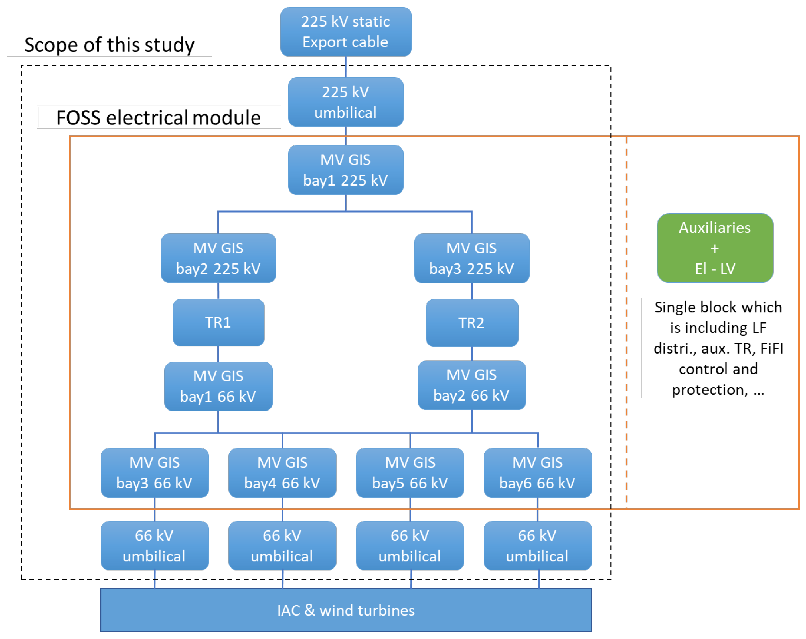
2.5. Main Blocks of a FOSS

The FOSS is composed of three main blocks of components from the reliability perspective: mooring and anchor system, floating platform and topside structure, and electro-technical subsystem. Under the availability assumption, these components are connected in series.

The electrical components of the FOSS are divided into two functional subsystems: the main power system and the auxiliary system (secondary functions). The main power system comprises MV/HV transformer(s), HV and MV switchgears (GIS), and an auxiliary transformer. The auxiliary system comprises equipment necessary to the main power system and to the substation in general to safely operate within the design operational conditions. The dynamic power cables (umbilical) can be considered as a member of electrical components, which is used to collect the power generated by the floating wind farm and to export it to the hub connecting to the static export cable that goes to the distribution center. Figure 1 represents the electrical configuration of the FOSS with a capacity of 250 MW.

The mechanical part of the FOSS involves the topside structure and the floating support, which consists of the floating platform and the mooring system. It must be noted that we only consider the mooring system’s reliability assessment within the mechanical components’ reliability analyses since the other parts are highly reliable. The substation is designed to be moored from the four corners of the floater by catenary mooring lines. In order to provide redundancy in case of the failure of a line, two configurations will be considered: 4 × 2 lines and 4 × 3 lines. Figure 2 illustrates the mooring system of the FOSS with two and three mooring lines for each corner.

2.6. Values of Component Failure Rates Considered for the Electro-Technical Components

Table 1. MTTF, MTTR, and failure rate of main electrical components.

Component	MTTF (Years)	MTTR (Days)	Failure Rate
GIS 66	50	21	0.002
GIS 225	50	21	0.002
Transformer	200	60	0.005
Umb 66	15–40	-	0.025–0.067
Umb 225	15–40	-	0.025–0.067

provides the required information for the components of the main power system. Preparing such information is straightforward using the feed-backs and statistical information collected by the owners.

It should be mentioned that the MTTF is provided according to minor failures, and the MTTR is provided according to major repairs. This leads to a conservative estimation of the reliability and availability levels of the system. Moreover, information about the MTTR and MTTF of the umbilical cable is provided according to the experts’ opinion.

3. Results

3.1. Values of Component Failure Rates Considered for the Mechanical Components

The design of mooring lines for offshore wind turbines does not always consider the redundancy of mooring systems [12]. Since the role of an FOSS is crucial for energy production, energy producers prefer designs with the redundancy of mooring lines, i.e., two or three, per anchoring point. From a reliability point of view, this redundancy is represented by a parallel system. Since these structures are at an early stage, it is not reasonable to perform a detailed reliability analysis for which quite a lot of assumptions are required. A more pragmatic approach relies on the feedback of past failures of mooring lines in a mature industry (floating oil and gas offshore industry) [13]. This approach is consistent with the estimation of failure rates of other components of the FOSS. It accounts for all failure modes, avoiding the discussion of the competition between failure modes and the occurrence of the demand: corrosion, fatigue, corrosion under stress, and extreme events. Such approaches are available in [12,14,15] for offshore wind turbine, but the failure rates cannot be extrapolated to a Floating Offshore Wind Turbine (FOWT) since the movement of an FOWT is much less as well as the effect of wind on the loading. Other studies have been carried out for Floating Production Storage and Offloading vessels (FPSOs) [16]; they cannot be used as well, because their hydrodynamic behavior differs significantly due to the difference of size (FPOSO is much larger) and due to the difference of mooring system (close to a single-point mooring for an FPSO).

From this feedback, the annual probability of failures $p_{rex}$ of similar but larger systems is available. The challenge is then to assess the reliability of a parallel system for intact or partially failed conditions. The following sections propose an efficient way for assessing this system’s reliability of the FOSS from the knowledge of the annual probability of failure of a line $p_{rex}$. The first objective for reliability analysis is to obtain unknown parameters (in intact and damaged conditions) by knowing $p_{rex}$. This can be achieved using a simple limit state (Equation (20)) that includes all the failure cases.

$$G(R,F)=R-F$$

(20)

where R and F denote, respectively, the resistance and the loading

Intact condition: As discussed in Section 2.3, the failure rate of the mechanical system (mooring line) can be obtained using Equation (17). However, one needs to calculate the values of $p_f$ and $P_f\left(T\right)$. For that reason, we model the loads $F_1$ and $F_2$ on the mooring lines and their resistance R with random variables without dimension. The events $\{R\le F_1\}$ and $\{R\le F_2\}$ obtained from the static equilibrium are nested, meaning that the failure of lines will happen in an order since $F_1\le F_2$ (see Figure 3). It is assumed that the resultant environmental loading F is perpendicular to the y-axis and acts on one side of the FOSS. Moreover, it is assumed that all lines have the same material properties, and dimensions, and the mooring pattern is symmetrical.

The environmental loading F is modeled with a random variable that follows a log-normal distribution with a known mean ${\mu }_F$ and unknown standard deviation ${\sigma }_F$. We assume that the material breaking strength R has a fixed standard deviation ${\sigma }_R$. It is given as a percentage of the maximum breaking load ${\mu }_R=1.1$ that does not change during the period of service, and is chosen to satisfy the fatigue strength in both conditions intact and damage. In what follows, we consider that R has a coefficient of variation of $C{V}_R=20\%$. The mean value and the variance of load F can be estimated using a sample of the annual failure probability of one line $p_{rex}$. The total failure probability of the system is then approximated using this uncertainty on the environmental load.

The material breaking strength is approximated by a log-normal distribution. In what follows, environmental load F and material strength R are both modeled with log-normal random distribution. Knowing the statistics for the environmental loading, static equilibrium can be simply used to evaluate the magnitudes of ${\mu }_i$, ${\sigma }_i$. The static equilibrium in x direction writes:

$$F_{1}cos\left({\theta }_1\right)+F_{2}cos\left({\theta }_2\right)=\frac{F}{2}$$

(21)

Further, under the assumption of small displacements, one can write: $F_{1}cos\left({\theta }_2\right)=F_{2}cos\left({\theta }_1\right)$. By injecting this information in previous equation, we obtain:

$$F_1=\frac{Fcos\left({\theta }_1\right)}{2(cos{\left({\theta }_1\right)}^2+cos{\left({\theta }_2\right)}^2)}$$

(22)

$$F_2=\frac{Fcos\left({\theta }_2\right)}{2(cos{\left({\theta }_1\right)}^2+cos{\left({\theta }_2\right)}^2)}$$

(23)

Hence, the standard deviation ${\sigma }_1$ and ${\sigma }_2$ can be calculated by the following equations:

$${\sigma }_1=\frac{{\sigma }_{R}cos\left({\theta }_1\right)}{2(cos{\left({\theta }_1\right)}^2+cos{\left({\theta }_2\right)}^2)}$$

(24)

$${\sigma }_2=\frac{{\sigma }_{R}cos\left({\theta }_2\right)}{2(cos{\left({\theta }_1\right)}^2+cos{\left({\theta }_2\right)}^2)}$$

(25)

Further, the coefficients of variation satisfy $C{V}_{F_i}=\frac{\sigma }{{\mu }_F}$.

The failure probability $p_i=P(R-F_i\le 0)$ computes the probability that line i breaks $(i=1,2)$, and it writes:

$$p_i\left(\sigma \right)={\int }_0^{\infty }{\mathsf{\Phi }}_R\left(r\right){\varphi }_{F_i}\left(r\right)dr$$

(26)

where ${\varphi }_{F_i}$ is the probability density function (pdf) of the load $F_i$, and ${\mathsf{\Phi }}_R$ is the cumulative density function (CDF) of the strength R. The quadrature method is used to estimate the integral (26) in order to obtain an accurate estimation. Further, $p_i\left(\sigma \right)$ is a monotonous function of $\sigma$; therefore, from a sample value $p_{rex}$, its corresponding value $\sigma$ is given by inverting the equation $\sigma =p_i^{-1}\left(p_{rex}\right)$.

Damaged condition: Here, we consider the case in which one line is damaged. From the nested loading case, $l_2$ will break first. The remaining load on Line 1 is denoted by $F_1^{\prime }$, where probably $F_1<F_1^{\prime }$ (see Figure 4). It is assumed here that the remaining non-damaged lines are loaded according to Equations (22) and (23) (Assumption 2). Therefore, the projection of the static equilibrium on the x-axis writes:

$$F_1^{\prime }cos\left({\theta }_1\right)+F_{1}cos\left({\theta }_1\right)+F21cos\left({\theta }_2\right)=F$$

(27)

Equations (22) and (23) are substituted in Equation (27) in order to obtain:

$$F_1^{\prime }=\frac{F}{2cos\left({\theta }_1\right)}$$

(28)

This equation shows also that $F_1^{\prime }$ follows a log-normal distribution with mean ${\mu }_{F_1^{\prime }}=\frac{\mu }{2cos\left({\theta }_1\right)}$ and standard deviation ${\sigma }_{F_1^{\prime }}=\frac{\sigma }{2cos\left({\theta }_1\right)}$, where $\sigma$ is computed from the intact condition case. Similarly, the failure probability of the second line $p_{1|2}=P(R-F_1^{\prime }\le 0)$ can be computed with the following integral:

$$p_{1|2}\left(\sigma \right)={\int }_0^{\infty }{\mathsf{\Phi }}_R\left(r\right){\varphi }_{F_1^{\prime }}\left(r\right)dr$$

(29)

where ${\varphi }_{F_1^{\prime }}$ is the pdf of the load $F_1^{\prime }$. It should be noted that the random variables $F_1^{\prime }$ and $F_2^{\prime }$ have the same coefficient of variation as load F. The probability of the damage of two lines satisfies $P(R\le F_1;R\le F_2)=P(R\le F_1)$ since $F_1\le F_2$ (nested load case).

The failure of the system is considered when two lines in the same corner are broken. Therefore, the total failure probability of the system $P_{FT}$ is calculated by:

$$\begin{array}{c}\hfill P_{FT}=P\left((l_1,l_2)or(l_1^{\prime },l_2^{\prime })arebroken\right)\\ \hfill =P(l_1,l_2)+P(l_1^{\prime },l_2^{\prime })-P\left(l_2\right)P\left(l_2^{\prime }\right|l_2)P\left(l_1^{\prime }\right|l_2,l_2^{\prime },l_1)\\ \hfill =2p_2{p}_{1|2}-p_2{p}_{1|2}{p}_F\end{array}$$

(30)

where by the symmetry and Assumption 2, we obtain $p_2=P\left(l_2^{\prime }\right|l_2)$, and the conditional probability $P\left(l_1\right|l_2,l_2^{\prime })=p_{1|2}$ holds true. The probability $p_F:=P\left(l_1^{\prime }\right|l_2,l_2^{\prime },l_1)$ is computed as in Equation (29) with stress F instead of $F_1$ or $F_2$ (it represents the damage probability of line $l_1^{\prime }$ given the damage of lines $l_1$, $l_2$, $l_2^{\prime }$).

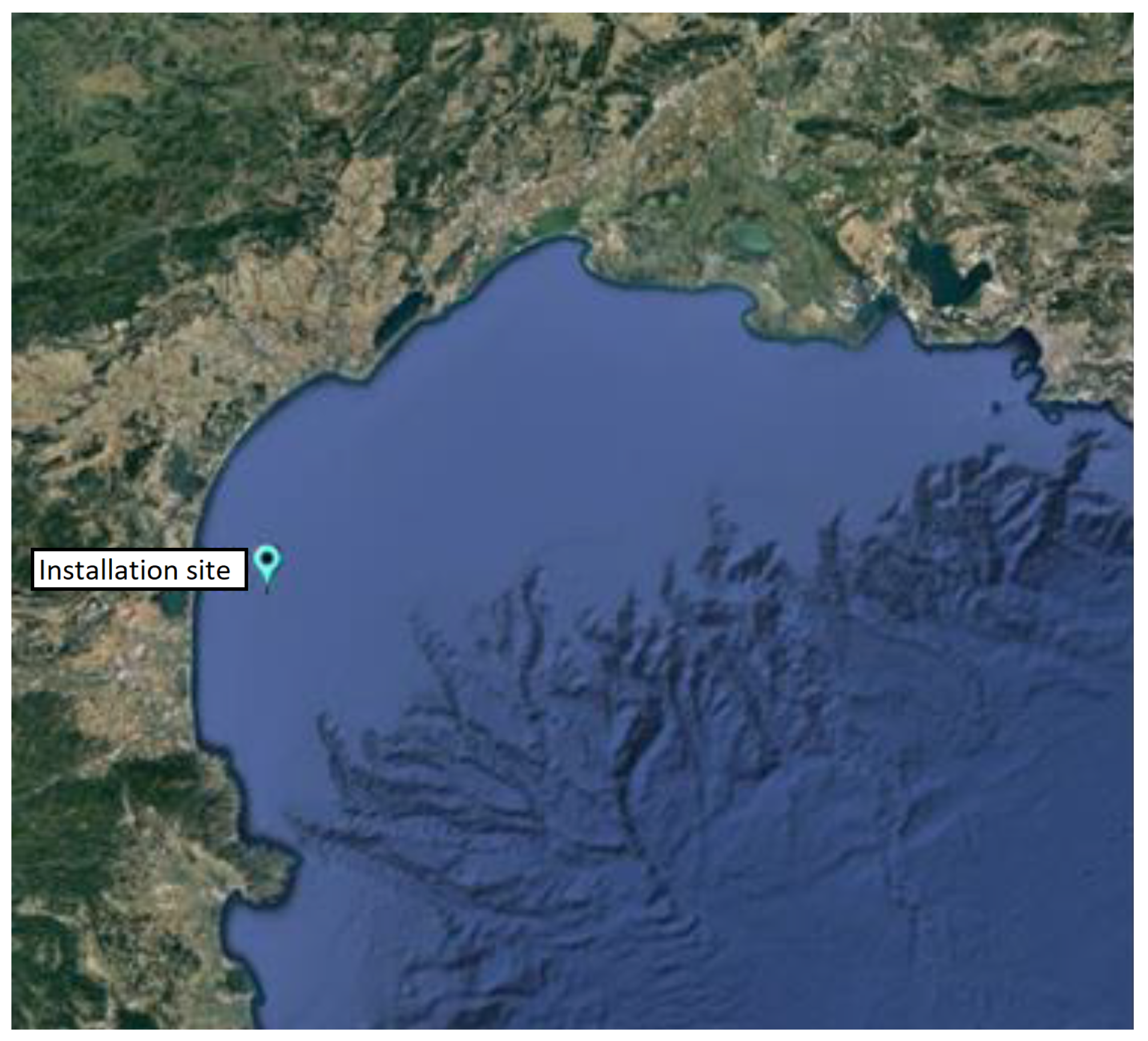
3.2. Installation Site

The installation site of the FOSS is “Golfe de Lion” in the Mediterranean Sea (see Figure 5). The estimated water depth of the installation site is 70–100 m. The project partner RTE (Réseau de Transport d’Électricité) provides the required information about the wave height and direction, wind speed and direction, sea current direction, etc. The provided information about the installation location is used to compute the loading F and design the mooring lines according to the standard using DeepLines software [17] according to DNV [18]. The mean values are used for estimation of $F_1$ and $F_2$.

4. Discussion

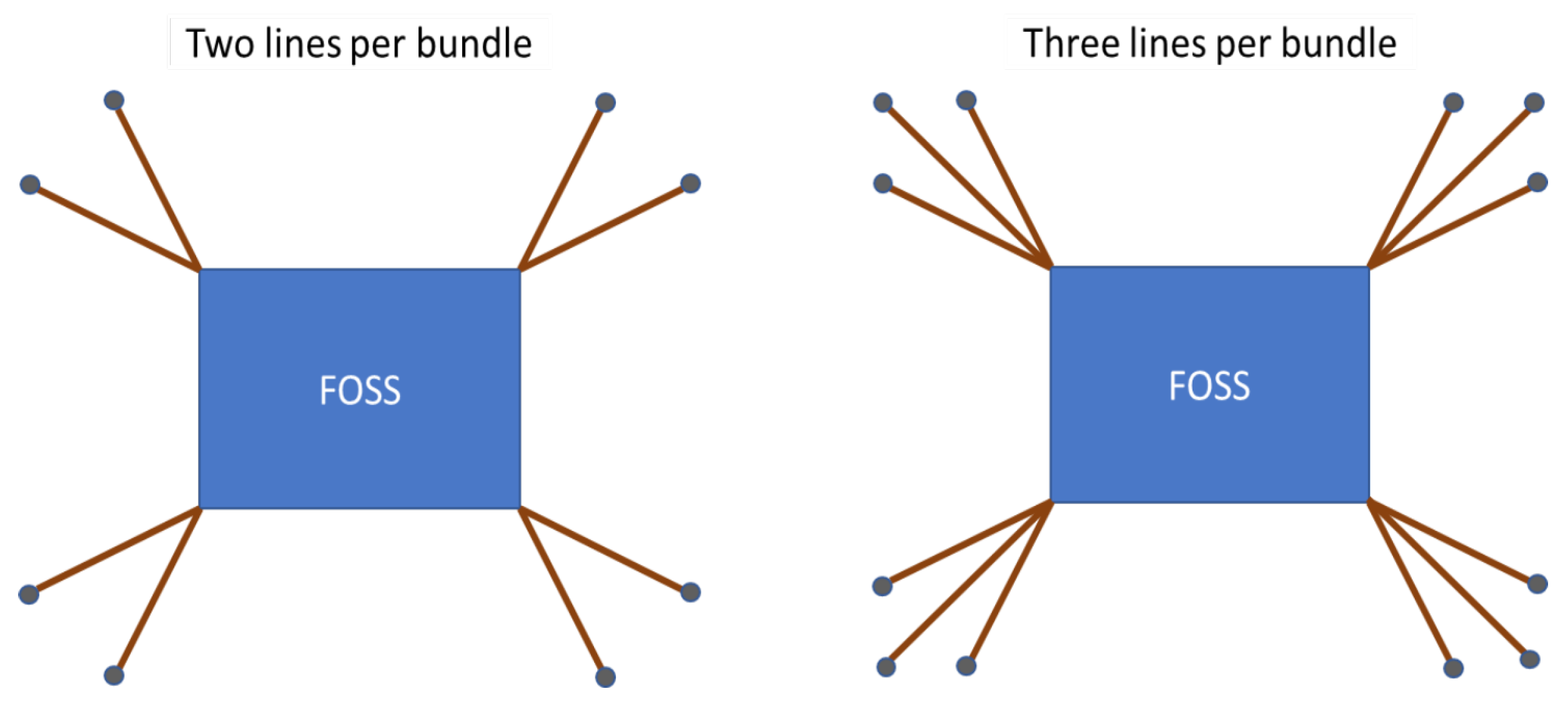
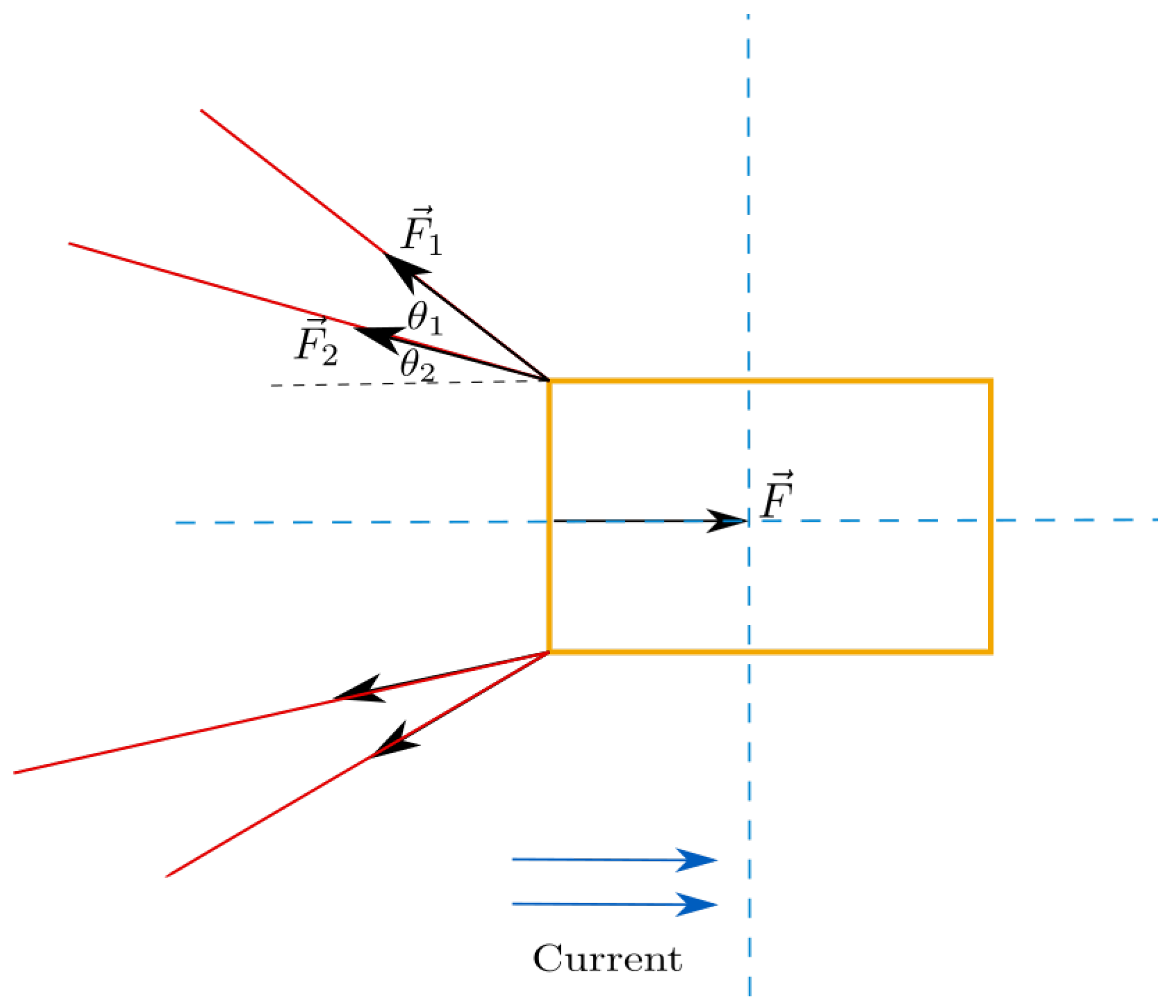
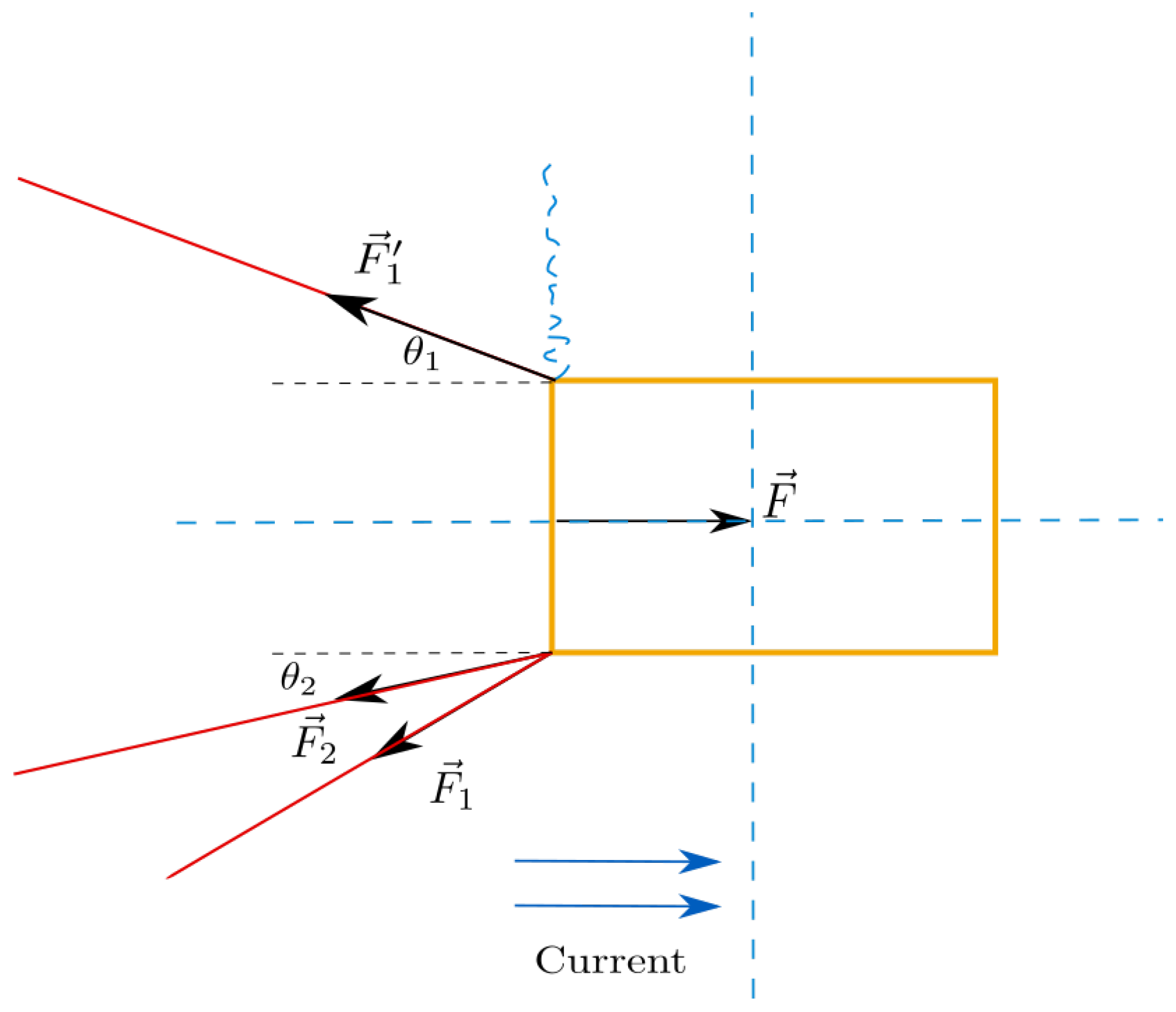
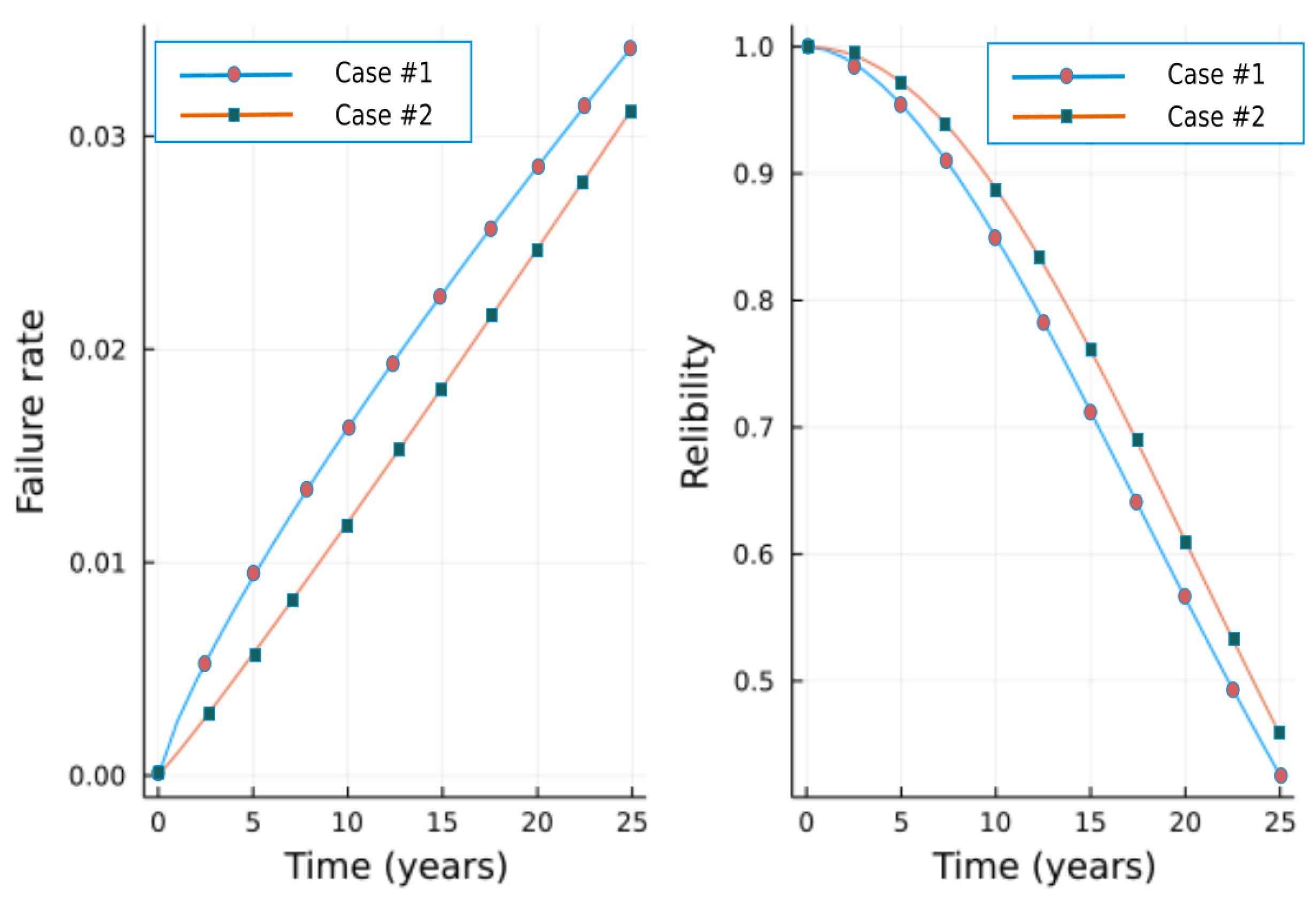
4.1. Mooring System Time-Variant Reliability Computation

A dynamic approach by DeepLines software is used in order to find the extreme tension in the mooring lines.

Table 2. Case study details.

Case	Substation	Mooring System	Design Tension (MPM) (Tons)	Condition
#1	SeeOS1XL 250 MW (2TR185/132MVA)	8 lines, chain, 100 mm RS4 Mooring radius: 900 m	497.3 772.8	Intact Damaged
#2	SeeOS1XL 250 MW (2TR185/132MVA)	12 lines, chain, 100 mm RS4 Mooring radius: 900 m	316.3 419.2	Intact Damaged

provides the MPM (most probable maximum) effort as calculated for both intact and damage conditions in each scenario. The design effort concerns the maximum tension on the upper lines ($l_1$, $l_2$) in the intact and damage conditions. The other lower lines $l_1^{\prime }$, $l_2^{\prime }$ are assumed to be loaded nearly like $l_1$, $l_2$, whereas the remaining lines on the other side are subjected to a very weak effort. We assume nested stresses $F_1<F_2$ with the same coefficient of variation $C{V}_F$. This coefficient is computed by inverting the equation $p_1=p_{rex}$, where $p_1$ is the failure probability of the line $l_1$. The failure probability of the system $P_{FT}$ is estimated by $P_{FT}\approx 2p_1{p}_{2|1}$. The probability $p_1$ is calculated using the lower and upper values $p_{rex}=0.005,0.02$. From these sample values, we deduce the $C{V}_F$ to compute the $p_{2|1}$. The material breaking strength R has a coefficient of variation of $C{V}_R=20\%$ and the mean ${\mu }_R$. This mean is equal to the minimum breaking load (MBL), which depend on the diameter of the chain of type $R4s$:

$${\mu }_R\left(R4s\right)=0.0304(44-0.08d)d^2$$

(31)

Table 3. Failure probabilities of mooring lines for considered cases.

Cases	#1	#2
${\mu }_R$ (tons)	1115.977	745.968
$C{V}_F$ (lower)	0.301	0.344
$C{V}_F$ (upper)	0.452	0.507
$p_{2|1}$ (lower)	0.140	0.0506
$p_{2|1}$ (upper)	0.204	0.101
$P_{FT}$ (lower)	0.0014	5.06 × 10${}^{-4}$
$P_{FT}$ (upper)	0.00818	0.004

provides the failure probabilities with lower and upper estimates of the $p_{rex}$ for two cases in Table 2. Equations (17) and (18) are used in order to calculate the failure rate of the mooring system, where $P_F:=p_f$, and two asymptotic estimates $P_f\left(T\right)=0.9,0.999$ are, respectively, used for the lower and upper estimates of $P_{FT}$ of the mooring system at time $T=60$ years.

Figure 6 shows the time-dependent curves of the failure rate and reliability of the mooring system with two and three lines per each corner. It can be easily observed that the mooring system with three mooring lines per corner leads to lower failure rates rather than having only two mooring lines per corner. This is reasonable since the loading on the mooring system is distributed on three mooring lines rather than two lines.

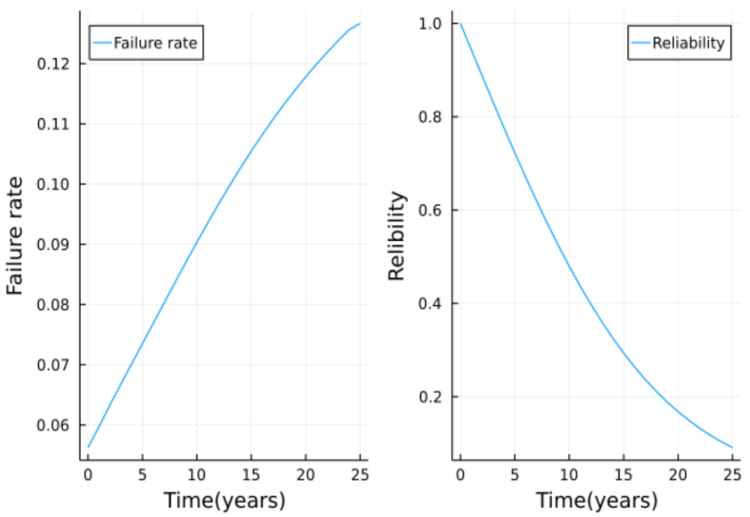
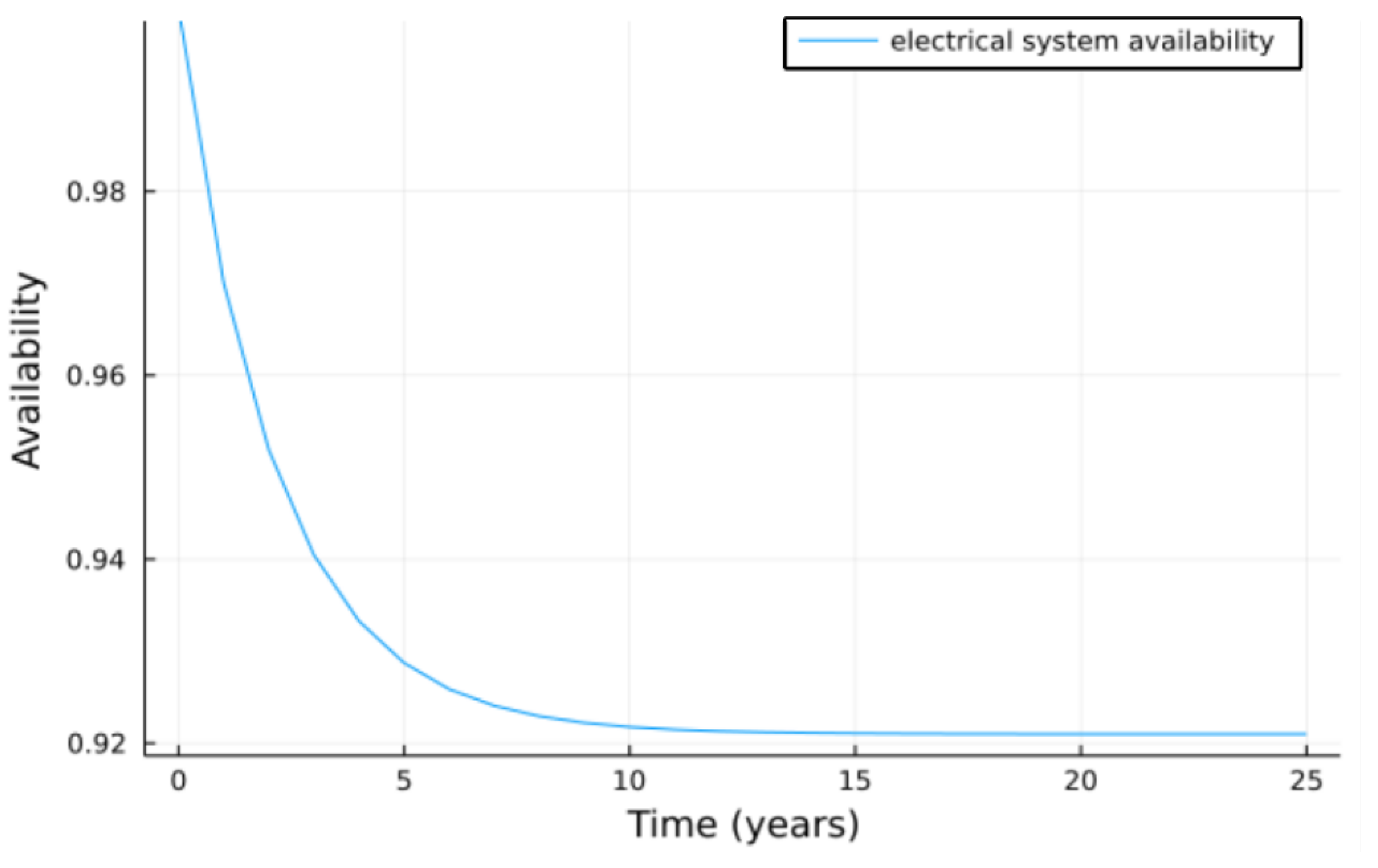
4.2. Electrical System Time-Variant Reliability Computation

In order to simplify the reliability computation of the electrical systems, it can be divided into serial and parallel subsystems. Figure 7 illustrates the failure rate and reliability curves of the main electrical system. It can be realized that the order of magnitude of the failure rates of the main electrical system is much higher than that for the mooring systems. On that account, the reliability level of the main electrical system decreases faster with time compared to the mooring system.

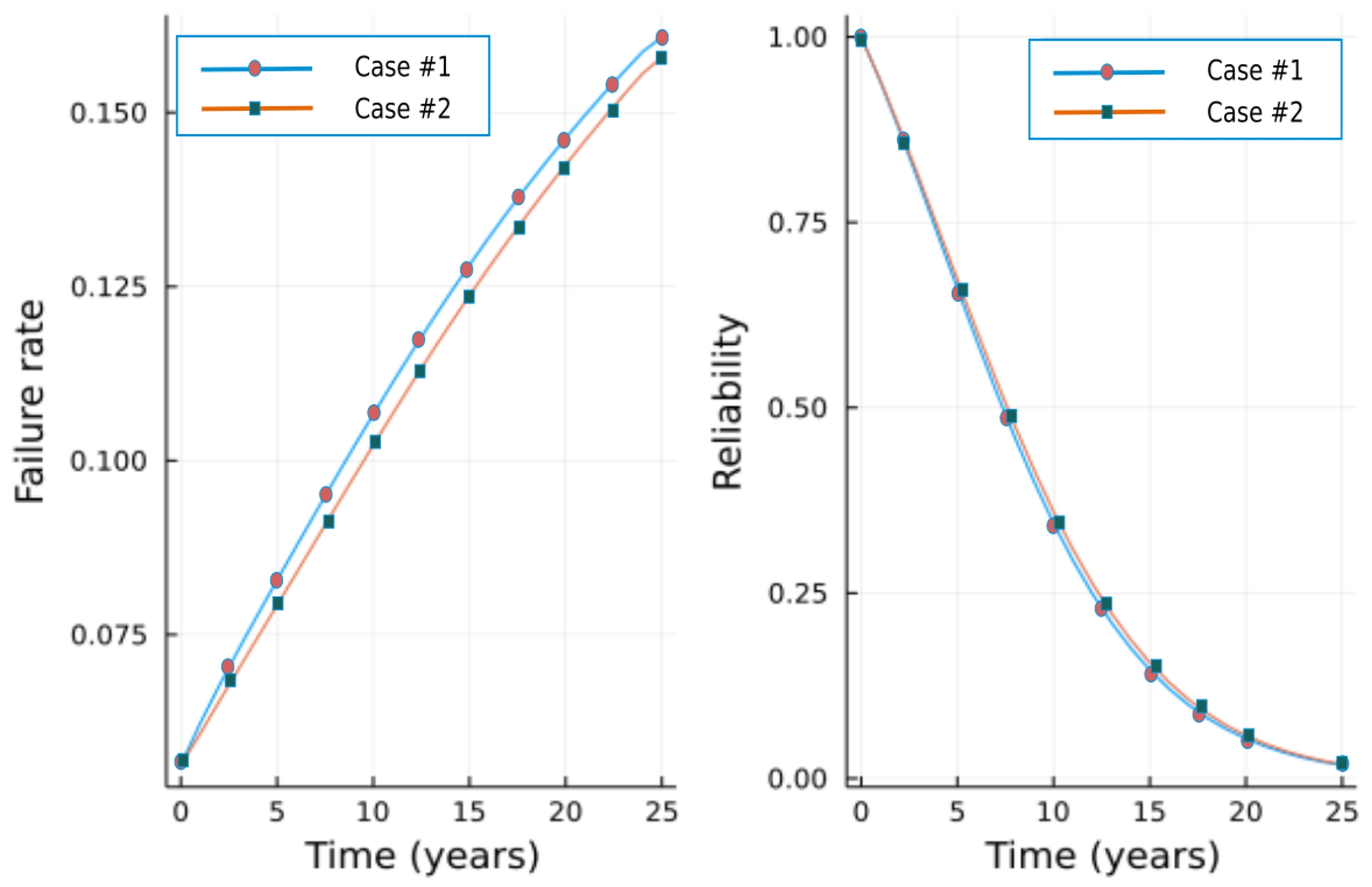
4.3. FOSS Electro-Mechanical Time-Variant Reliability Computation

Using the proposed unified approach, we can estimate the reliability of the FOSS. Figure 8 demonstrates the time-dependent failure rate and reliability curves of the FOSS. It can be seen that the order of magnitudes of the failure rates and reliability levels of the FOSS are close to the ones of the main electrical system. Therefore, it can be concluded that the main electrical systems have a more significant influence on the reliability of the FOSS. Another important conclusion in the section is that changing the mooring system from two lines per corner to three lines per corner does not make a big difference in the reliability levels of the FOSS.

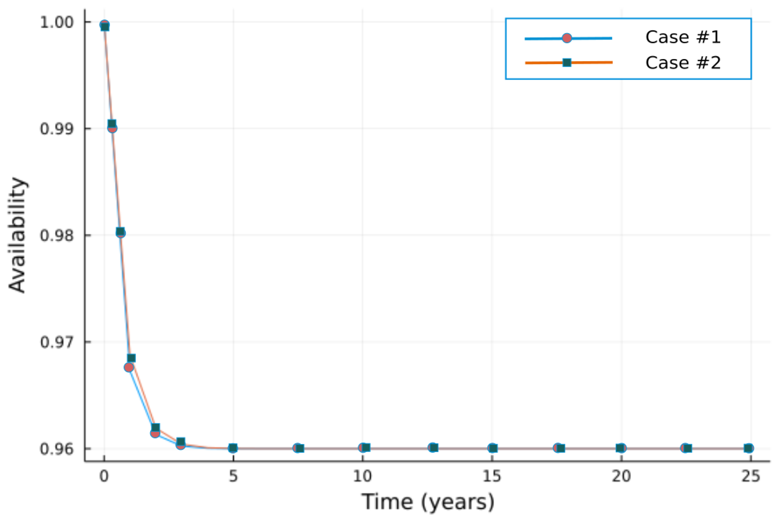
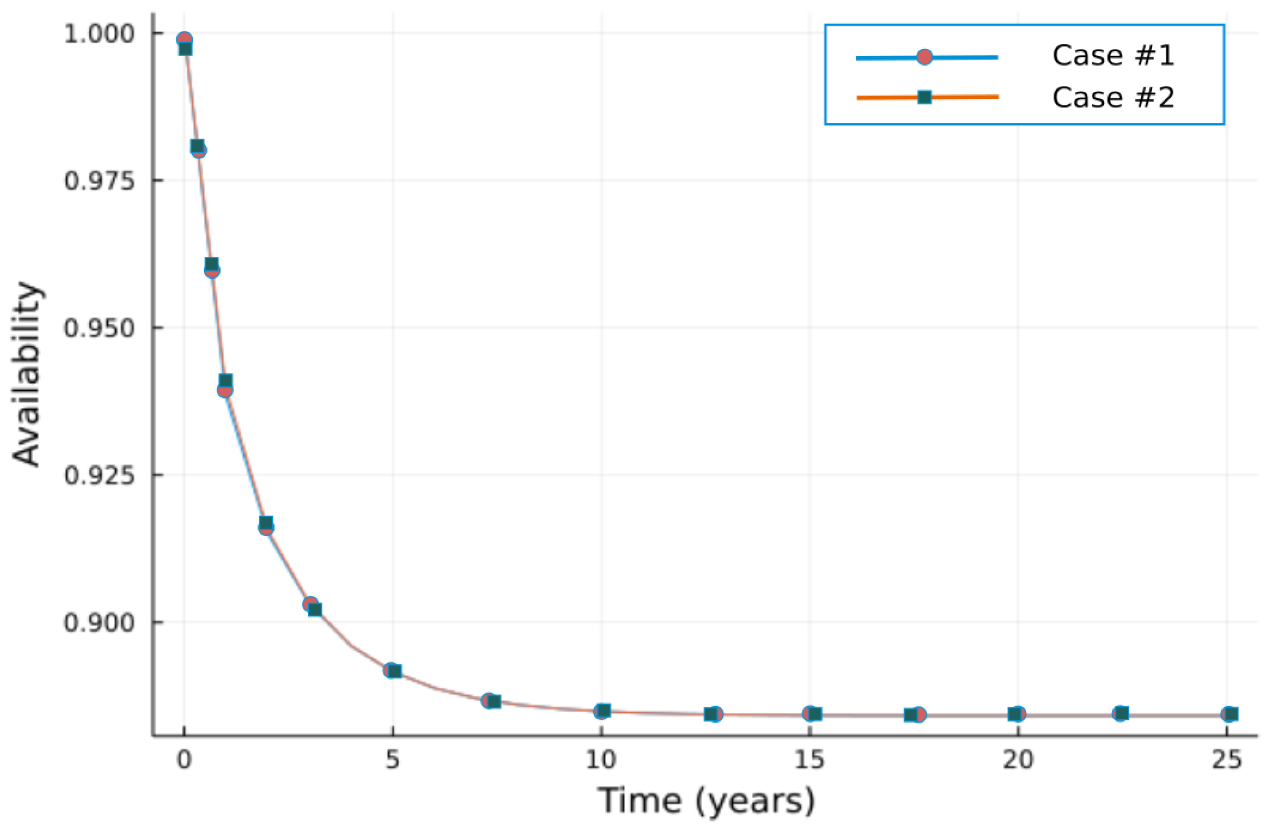
4.4. FOSS Availability Analysis

This section presents the results of the availability analysis for electrical, mooring systems, and the entire FOSS. Since there is a lack of information on the repair rate of the mooring system, it is assumed that the average availability for the mooring system is 0.96. Accordingly, one can use Equation (5) in order to calculate the repair rate of the mooring system. Equation (6) is then used to calculate the time-dependent availability of the mooring system.

Figure 9 shows the time-dependent availability curves for both mooring systems. It can be realized from this figure that both mooring systems (two lines and three lines per corner) have almost the same availability levels for different time nodes. It can also be seen that the availability of each mooring system converges to 0.96 after 5 years of its service life. This value has been assumed before for the average availability of mooring systems to obtain their repair rate values.

Table 4. MTTR for electrical components for major repair actions.

Component	MTTR (Days)
GIS 66 KV	21
GIS 225 KV	21
Transformer	60

provides the information for MTTR of electrical components for major repairs. Due to the lack of information on the MTTR of the umbilical cables, it is assumed that the MTTR (umbilical) = 1.5 MTTR (mooring). Hence, one can use Equation (6) to calculate the availability of the main electrical system. In this respect, Figure 10 shows the results of the availability analysis of the main electrical system. The average availability of the main electrical system is 0.92. The main electrical system needs 10 years of service life to converge to this value.

The final step is related to computing the availability of the FOSS. As previously mentioned, it can be assumed that the main electrical and mooring systems are serially connected. On that account, one can easily calculate the availability of the FOSS by knowing the availability of the mooring and the main electrical systems. Figure 11 illustrates the availability levels of the FOSS with both mooring strategies. It shows that the availability curves of the FOSS with different mooring systems are almost coinciding. Therefore, it can be concluded that mooring strategies do not make a sensible difference in the availability of the FOSS. Like the availability curve of the electrical system, the availability curve of the FOSS reaches its average value after almost 10 years of service life.

5. Conclusions

The main objective of this study was to assess the reliability and availability of a new type of offshore structure, the Floating Offshore Substation (FOSS), by performing reliability and availability analyses on its mechanical and electrical components. To this end, we proposed a unified approach for calculating the failure rate of the FOSS that takes into account both the electrical and mechanical subsystems. Specifically, we developed a new formulation to estimate the failure rate of mechanical components using the annual failure probability, which is a crucial step for evaluating the overall failure rate of the FOSS system and conducting reliability/availability analyses.

We also presented the configuration of the electrical components and their failure rates, as well as two mooring systems for the mechanical aspect, with one involving eight mooring lines and the other twelve. The FOSS installation site is located in the Mediterranean Sea on the coast of France.

To calculate the failure rate of the electrical system, we utilized the failure rates of individual electrical components and their arrangement in the system. The failure rate of the mooring system was estimated based on the loading conditions, resistance of mooring lines, and failure event. We then used the proposed unified approach to evaluate the overall failure rate of the FOSS system. Finally, we provided reliability and availability calculations for the electrical and mechanical subsystems, as well as the FOSS as a whole. Our results indicated that the electrical subsystem had a greater impact on the system’s reliability.

In conclusion, this study provides initial findings on the reliability and availability of the innovative FOSS. While our approach could be improved by obtaining better input data on dynamic cables and mooring lines, we believe that our proposed unified approach can be readily adopted to evaluate the reliability of the FOSS in other installation sites.

References

1. IEA Paris. World Energy Outlook; Technical report; IEA: Paris, France, 2019. [Google Scholar]
2. IRENA. Future of Wind: Deployment, Investment, Technology, Grid Integration and Socio-Economic Aspects; Technical report; International Renewable Energy Agency: Abu Dhabi, United Arab Emirates, 2019. [Google Scholar]
3. Firestone, J.; Bates, A.W.; Prefer, A. Power transmission: Where the offshore wind energy comes home. Environ. Innov. Soc. Transitions 2018, 29, 90–99. [Google Scholar] [CrossRef]
4. James, R.; Weng, W.; Spradbery, C.; Jones, J.; Matha, D.; Mitzlaff, A.; Ahilan, R.; Frampton, M.; Lopes, M. Floating Wind Joint Industry Project—Phase I Summary Report. Technical report, Carbon Trust report. 2018. [Google Scholar]
5. Oh, K.Y.; Nam, W.; Ryu, M.S.; Kim, J.Y.; Epureanu, B.I. A review of foundations of offshore wind energy convertors: Current status and future perspectives. Renew. Sustain. Energy Rev. 2018, 88, 16–36. [Google Scholar] [CrossRef]
6. Fukushima Offshore Wind Consortium. Fukushima Floating Offshore Wind Farm Demonstration Project (Fukushima FORWARD); Technical report, Fukushima FORWARD; The University of Tokyo: Tokyo, Japan, 2014. [Google Scholar]
7. Melchers, R.E.; Beck, A.T. (Eds.) Structural Reliability Assessment. In Structural Reliability Analysis and Prediction; John Wiley & Sons, Ltd.: Hoboken, NJ, USA, 2017. [Google Scholar] [CrossRef]
8. Availability and Maintainability in Engineering Design. In Handbook of Reliability, Availability, Maintainability and Safety in Engineering Design; Springer: London, UK, 2009; pp. 295–527. [CrossRef]
9. Ahmadivala, M.; Mattrand, C.; Gayton, N.; Orcesi, A.; Yalamas, T. AK-SYS-t: New Time-Dependent Reliability Method Based on Kriging Metamodeling. ASCE-ASME J. Risk Uncertain. Eng. Syst. Part A Civ. Eng. 2021, 7, 04021038. [Google Scholar] [CrossRef]
10. Amari, S.; Akers, J. Reliability analysis of large fault trees using the Vesely failure rate. In Proceedings of the Computer Science, Engineering Annual Symposium Reliability and Maintainability, 2004—RAMS, Los Angeles, CA, USA, 26–29 January 2004. [Google Scholar]
11. Rice, S. Mathematical Analysis of Random Noise; Bell Telephone System, Technical publications; Monograph; American Telephone and Telegraph Company: Dallas, TX, USA, 1944. [Google Scholar]
12. Pham, H.D.; Schoefs, F.; Cartraud, P.; Soulard, T.; Pham, H.H.; Berhault, C. Methodology for modeling and service life monitoring of mooring lines of floating wind turbines. Ocean Eng. 2019, 193, 106603. [Google Scholar] [CrossRef]
13. Ma, K.T.; Shu, H.; Smedley, P.; L’Hostis, D.; Duggal, A. A Historical Review on Integrity Issues of Permanent Mooring Systems. In Proceedings of the Offshore Technology Conference, Houston, TX, USA, 6–9 May 2013. [Google Scholar] [CrossRef]
14. Zhao, G.; Zhao, Y.; Dong, S. System reliability analysis of mooring system for floating offshore wind turbine based on environmental contour approach. Ocean Eng. 2023, 285, 115157. [Google Scholar] [CrossRef]
15. Li, H.; Peng, W.; Huang, C.G.; Guedes Soares, C. Failure Rate Assessment for Onshore and Floating Offshore Wind Turbines. J. Mar. Sci. Eng. 2022, 10, 1965. [Google Scholar] [CrossRef]
16. Wang, Y.; Zou, C.; Ding, F.; Dou, X.; Ma, Y.; Liu, Y. Structural Reliability Based Dynamic Positioning of Turret-Moored FPSOs in Extreme Seas. Math. Probl. Eng. 2014, 2014, 302481. [Google Scholar] [CrossRef]
17. Magazine, R.E. IFPEN and Principia release DeepLines Wind FEA software. 2015. [Google Scholar]
18. DNV. Recommended Practice DNV-RP-C205: Environmental Conditions and Environmental Loads; Technical report; Det Norske Veritas: Bellum, Norway, 2010. [Google Scholar]
Figure 1. One module, two transformers per module (250 MW).
Jmse 11 01924 g001
Figure 2. FOSS mooring systems.
Jmse 11 01924 g002
Figure 3. Loading conditions on mooring lines (intact condition).
Jmse 11 01924 g003
Figure 4. Loading conditions on mooring lines (damaged condition).
Jmse 11 01924 g004
Figure 5. FOSS installation site in the Mediterranean Sea on the coast of France.
Jmse 11 01924 g005
Figure 6. The failure rate and reliability (lower bound) of the mooring system for each scenario.
Jmse 11 01924 g006
Figure 7. Failure rate and reliability curves for the main electrical system.
Jmse 11 01924 g007
Figure 8. The failure rate and reliability of the FOSS.
Jmse 11 01924 g008
Figure 9. Availability of the mooring system.
Jmse 11 01924 g009
Figure 10. Availability of the main electrical system.
Jmse 11 01924 g010
Figure 11. Availability of the FOSS.
Jmse 11 01924 g011