Three-Dimensional Modeling of Sound Field Holograms of a Moving Source in the Presence of Internal Waves Causing Horizontal Refraction

Abstract

In this paper, we study the variations of holograms of a moving source in an inhomogeneous ocean waveguide. It is assumed that intense internal waves (internal solitons) are the reason for the inhomogeneities of the shallow water waveguide. The results of 3D modeling of the sound field considering horizontal refraction by internal waves are presented. In the context of 3D modeling, the interferogram (sound intensity distributions in frequency–time coordinates) and hologram (2D Fourier transform of the interferogram) of moving sources are analyzed. The hologram consists of two disjoint regions corresponding to the unperturbed field and the field perturbed by internal waves. This structure of the hologram allows for the reconstruction of the interferogram of the unperturbed field in a waveguide in the absence of intense internal waves. The error in the reconstruction of the unperturbed interferogram is estimated.

1. Introduction

Currently, there is a great scientific interest in interferometric signal processing in underwater acoustics. The interferometric signal processing (ISP) is based on stable features of the interference structure (pattern) of the broadband sound field in the shallow water waveguide [1,2]. We refer the interested reader to the main work [3,4,5] on ISP methods. In papers [6,7], ISP is developed for estimating invariant parameters of waveguides. In work [8], ISP is applied to estimate invariant parameters for weak signals due to amplification of signal levels by array beamforming. In work [9], the ISP is used to classify the seabed based on the passing ship signals. In work [10], the ISP is offered to estimate the source range in shallow water. The ISP is used in work [11] for a range-independent invariant estimation. The ISP approach is used in paper [12] to explain interference fringes by eigenray arrival times. The ISP is developed in papers [13,14] for deep-sea passive sonar.

One of the most advantageous approaches of ISP is holographic signal processing (HSP) [15,16]. The physical and mathematical principles of hologram formation were first described in [15]. In HSP, the quasi-coherent accumulation of the sound intensity distribution in frequency–time coordinates (interferogram $I(\omega ,t)$) occurs [16]. A 2D Fourier transform (2D-FT) is applied to the accumulated sound intensity of the interferogram $I(\omega ,t)$. The 2D-FT of the interferogram $I(\omega ,t)$ is called a Fourier hologram (hologram) $F(\tau ,\tilde{\nu })$. The hologram $F(\tau ,\tilde{\nu })$ allows one to concentrate the sound intensity of the interferogram $I(\omega ,t)$ due to the interference of the different modes in focal spots.

In the development of HSP, it was assumed that waveguide parameters are constant in space and time coordinates. However, in many cases, acoustic signals propagate in waveguides with hydrodynamic perturbations. The HSP was first considered for non-moving source experimentally in paper [17]. It was shown that the hydrodynamic perturbations of the waveguide leads to a distortion of the interferogram $I(\omega ,t)$ and an increase of the focal spots in the hologram $F(\tau ,\tilde{\nu })$. In an inhomogeneous waveguide, the hologram $F(\tau ,\tilde{\nu })$ is represented as a superposition of two hologram components. These components consist of a hologram component related to the source in the unperturbed waveguide and a hologram component due to the waveguide perturbation. In [17], the HSP in inhomogeneous waveguides was applied to analyze the experimental data obtained in the SWARM’95 (1995) experiment [18,19]. The waveguide inhomogeneities during the SWARM’95 experiment are due to intense internal waves (IIWs) [19,20,21,22]. IIWs are a hydrodynamic phenomenon, which is widespread in the oceanic environment [20,21,22]. The presence of IIWs causes significant horizontal refraction of the sound field, which arises at a small angle to the wavefront of the IIWs [23].

The aim of this work is to present the results of theoretical analysis and numerical modeling of HSP for a moving source and a non-moving receiver in the presence of IIWs causing significant horizontal refraction. The IIWs influence on the error of the source parameters estimations (range, velocity, and movement direction) are analyzed.

Our research is based on numerical modeling of the sound field in three-dimensional (3D) inhomogeneous waveguides. Three-dimensional inhomogeneities of the propagation medium can significantly affect the structure of the sound field due to horizontal reflection, refraction, scattering, and diffraction. Numerical modeling of a broadband sound field in a 3D inhomogeneous waveguide is indeed a complex task and requires significant computational resources. To achieve accurate and realistic simulations of the sound field structure, advanced numerical techniques and high-performance computer systems are often required. The numerical algorithms for sound field modeling in inhomogeneous waveguides can be divided into four main groups [24]: 3D Helmholtz equation (3DHE) models [25,26,27]; 3D parabolic equation (3DPE) models [28,29,30,31,32]; vertical modes and 2D modal parabolic equations (VMMPE) models [23,33,34,35,36]; and 3D ray (3DR) models [37,38,39]. In the context of our study, we consider a low-frequency sound field ($\Delta f_1=$ 100–120 Hz; $\Delta f_2=$ 300–320 Hz). IIWs are assumed to be the reason for the inhomogeneities of the shallow water waveguide. We assume that the wavefront of IIWs is aligned along the acoustic track (source–receiver). In this case, the IIWs cause significant horizontal refraction of the acoustic waves, which are at a small angle to the wavefront of the IIWs. To account for the horizontal refraction of a low-frequency sound field in a shallow water waveguide, VMMPE is the most appropriate of the four models noted above. In the context of numerical modeling, the VMMPE model enables the solution of two important problems. The VMMPE sound field model accounts for the conditions at the boundaries of the shallow water waveguide and the horizontal refraction of the vertical modes. Unlike VMMPE, the 3DR model is not suitable for low-frequency sound fields in shallow-water waveguides. Due to its approximate nature, ray-tracing theory is more suitable at high frequencies. Compared to VMMPE, the 3DHE and 3DPE models are too complex for the case of a shallow water waveguide with IIWs considered in our work. They require extensive computational resources. For this reason, the numerical simulation in our work is based on the VMMPE model.

In our simulation, the shallow water waveguide with spatially and temporally varying parameters due to IIWs is used. The main assumption of our simulation is the following. The propagation velocity of sound waves (∼1500 m/s) from the source to the receiver is much larger than the source motion velocity (∼0.5–5 m/s) and the propagation velocity of IIWs (∼0.5–1 m/s). Therefore, we use the “frozen propagation environment” assumption [39,40]: the propagation environment is not changed during the time interval of propagation of sound waves from the source to the receiver.

The numerical implementation of the VMMPE model used in the work was developed in MATLAB [23]. The numerical implementation of the VMMPE model was verified using experimental data from SWARM’95 [41].

The paper consists of six sections. After the introduction in Section 1, we describe in Section 2 the 3D model of a shallow water waveguide in the presence of IIWs. Next, we derive the mathematical models of the interferogram $I(\omega ,t)$ in Section 3 and the hologram $F(\tau ,\tilde{\nu })$ in Section 4 of a moving source in a shallow water waveguide in the presence of the IIWs. The algorithm of the numerical calculation of the interferogram and hologram of moving source is developed. It is based on VMMPE model. The proposed algorithm allows us to take into account the horizontal refraction of the sound field caused by IIWs propagating across the acoustic track (source–receiver). The results of the numerical modeling of the interferogram $I(\omega ,t)$ and hologram $F(\tau ,\tilde{\nu })$ of the broadband sound source in the shallow water waveguide in the presence of IIWs causing horizontal refraction are analyzed in Section 5. Within the numerical modeling, the influence of IIWs on the interferogram $I(\omega ,t)$ and hologram $F(\tau ,\tilde{\nu })$ of the source sound field is considered for two different cases of source parameters. The first case is a stationary acoustic track source–receiver (non-moving source). The second case is a non-stationary acoustic trace (moving source). In order to compare the numerical modeling results for both cases in the presence of IIWs, the initial data for the simulation are chosen to be the same. The IIWs influence on the error of the source parameters estimates (range, velocity) are analyzed. In Section 6, the presented results are summarized.

2. Shallow Water Waveguide Model

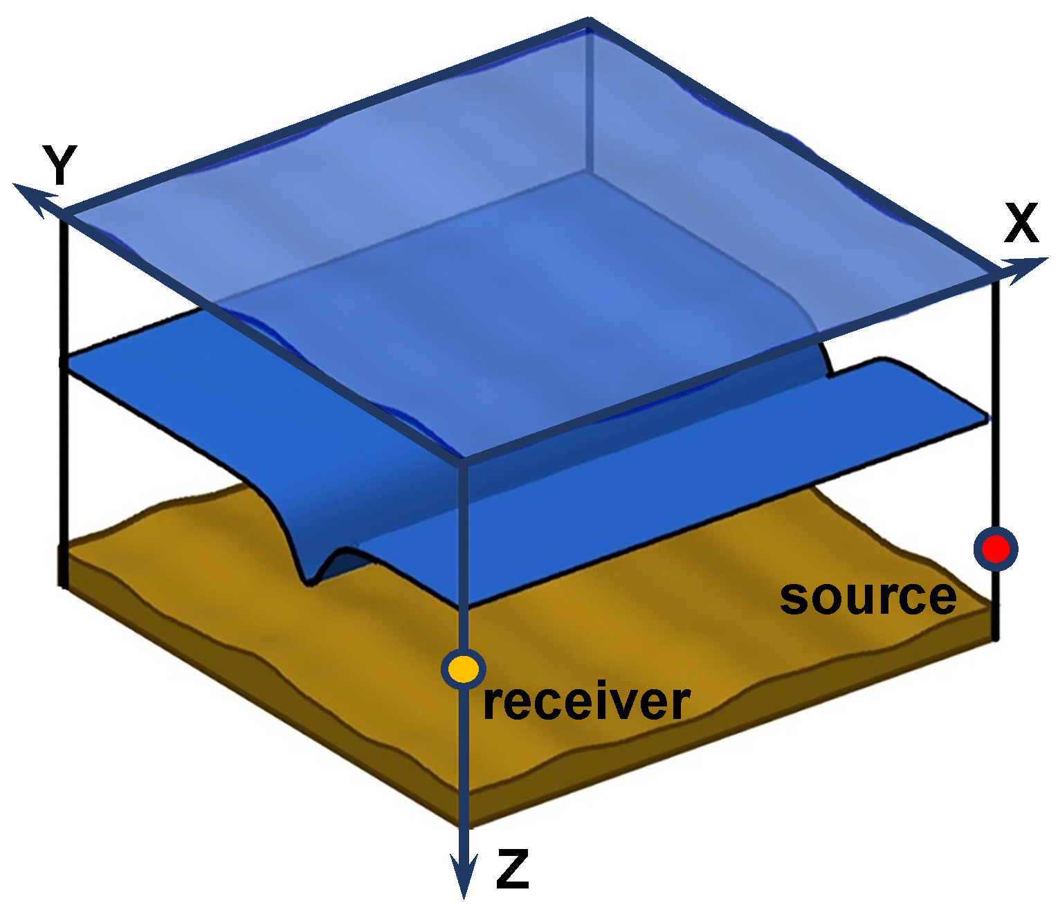
In this section, we describe the 3D model of the shallow water waveguide used in our research (Figure 1). The waveguide in coordinate system $(X,Y,Z)$ is represented as a water layer with a sound velocity $c(\mathbf{r},z,t)$ and a density $\rho (\mathbf{r},z,t)$. Here, $\mathbf{r}=(x,y)$ is the radius vector in the horizontal plane. The water layer is confined in depth by a free surface $(z=0)$ and the sea bottom ($z=H$).

The bottom density and refractive index are denoted by $n_b(1+\mathrm{i}\varkappa )$, ${\rho }_b$ [39,40], where $\varkappa =\chi c_b/54.6f$. Here, $\chi$ is a bottom loss coefficient, $c_b$ is the bottom sound speed, and f is the sound frequency. The space–time dependence of the sound velocity in the water can be represented in the following form:

$$c(\mathbf{r},z,t)=c\left(z\right)+\delta c(\mathbf{r},z,t),$$

(1)

where $c\left(z\right)$ is the velocity profile in the waveguide in the absence of the IIWs, and $\delta c(\mathbf{r},z,t)$ is the sound speed variations due to the IIWs. According to Equation (1), the squared refractive index in the water layer is

$$n^2(\mathbf{r},z_q,t)={\overline{n}}^2\left(z\right)+{\tilde{n}}^2(\mathbf{r},z,t),$$

(2)

where ${\overline{n}}^2\left(z\right)$ corresponds to the unperturbed waveguide, and ${\tilde{n}}^2(\mathbf{r},z,t)$ is due to IIWs.

According to [22,23], we have

$${\tilde{n}}^2(\mathbf{r},z,t)=-2Q{N}^2\left(z\right)\zeta (\mathbf{r},z,t).$$

(3)

Here, $Q\approx 2.4$ s${}^2$/m is a physical constant of water; $N\left(z\right)={(g{\rho }^{-1}d\rho /dz)}^{1/2}$ is the buoyancy frequency, and $\zeta (\mathbf{r},z,t)$ are the vertical displacements in the water layer due to IIWs. According to the first gravity mode predominance [20,21,22], $\zeta (\mathbf{r},z,t)$ can be expressed as follows:

$$\zeta (\mathbf{r},z,t)={\Phi }_1\left(z\right){\zeta }_0(\mathbf{r},t),$$

(4)

where ${\Phi }_1\left(z\right)$ denotes the eigenfunction of the first gravity mode, normalized at depth $z_0$: ${\Phi }_1\left(z_0\right)=1$; and ${\zeta }_0(x,y,t)$ are vertical displacements in the waveguide water layer due to IIWs at depth $z_0$.

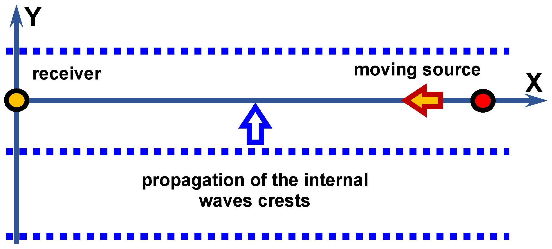
According to [20,21,22], we can represent IIWs as the sequence of internal solitons (IS—soliton-like solution of KdV-equation). Given the chosen problem geometry (Figure 2), the vertical displacements in the water layer of the waveguide ${\zeta }_0(\mathbf{r},t)$ can be described as

$${\zeta }_0(\mathbf{r},t)=\sum _{n=1}^N-B_n{sech}^2\left[(y-D_n-u_{n}t)/{\eta }_n\right],$$

(5)

where N is the count of the IS in train, $B_n$ is the IS amplitude, $u_n$ is the IS velocity, $D_n$ is the IS shift in horizontal plane, and ${\eta }_n$ is the IS width.

IIWs are widespread phenomenon in the ocean. They are trains of short-period vertical displacements of water layers. They are described as trains of IS that propagate to the shelf coast. The reason for the IIWs are internal tides [20,21,22]. According to experimental data [18,19,20,21,22], the parameters of IIWs are the following:

• Train length: ∼ 3–5 km ($N\sim$ 4–7);
• $\zeta$ has quasi-sinusoidality form (narrow spatial spectrum);
• $\zeta$ are synchronized in depth (dominance of the ${\Phi }_1\left(z\right)$);
• Propagation velocity: $u_n\sim$ 0.5–1 m/s;
• IS amplitude: $B_n\sim$ 10–30 m;
• IS width: ${\eta }_n\sim$ 100–200 m;
• Interval between IS: ∼ 300–500 m;
• Curvature radius of IS front in horizontal plane ∼ 15–25 km.

These parameters lead to specific acoustic phenomena due to IIWs. In [23,41], it is shown that the presence of IIWs causes significant horizontal refraction of sound waves, which are at a small angle to the wavefront of the IIWs. As a result, the dynamic waveguides in the horizontal plane are approximately parallel to the fronts of the IIWs. The sound intensity is periodically focused and defocused along the IIW front. This leads to significant variations in sound intensity (∼4–5 dB) at the receiver [23,41]. Within the VMMPE model [23,33,34,35,36], it is shown that horizontal dynamic waveguides have selective character for vertical modes. The horizontal structure of the sound field is different for different vertical modes. It is shown that the horizontal structure of the sound field of sound modes also depends on the frequency [23]. This frequency dependence of horizontal refraction has a resonance-like form and is evident in the propagation of broadband sound signals.

3. Moving Source Interferogram

In the framework of the VMMPE approach, the complex field in the waveguide in the presence of the IIW Equations (1)–(5) can be written in the following way [23,39,40,42]:

$$p(\mathbf{r},z,\omega ,t)=\sum _{m=0}^M{P}_m(\mathbf{r},\omega ,t){\varphi }_m(z,\omega )exp\left[\mathrm{i}({\overline{h}}_m+\mathrm{i}{\overline{\gamma }}_m)x\right],$$

(6)

where $\mathbf{r}=(x,y)$ is the radius vector of the source in the horizontal plane, $P_m$ is the mode amplitude, ${\overline{h}}_m+\mathrm{i}{\overline{\gamma }}_m$ is the complex horizontal wavenumber of the mth acoustic mode, and ${\varphi }_m(z,\omega )$ is the corresponding acoustic mode in the waveguide without IIWs. In Equation (6), the summation is performed up to M, the total number of acoustic modes to be considered. Consequently, the acoustic pressure depends on the acoustic frequency $\omega =2\pi f$.

The ${\varphi }_m(\mathbf{r},\omega ,t)$ are the eigenfunctions (acoustic modes), and $h_m(\mathbf{r},\omega ,t)$ and ${\gamma }_m(\mathbf{r},\omega ,t)$ are the real/imaginary parts of horizontal wavenumbers ${\xi }_m\left(\omega \right)=h_m(\mathbf{r},\omega ,t)+\mathrm{i}{\gamma }_m(\mathbf{r},\omega ,t)$, calculated by solving the Sturm–Liouville problem under conditions for free surface and bottom [39,40]. The horizontal wavenumber $h_m(x,z,t)$ of the mth acoustic mode in the presence of IIWs can be written as the sum of the unperturbed component (${\overline{h}}_m\left(\omega \right)$) and the perturbation ${\tilde{h}}_m(\mathbf{r},\omega ,t)$ due to IIWs:

$$h_m(\mathbf{r},\omega ,t)={\overline{h}}_m\left(\omega \right)+{\tilde{h}}_m(\mathbf{r},\omega ,t).$$

(7)

The linear correction in (7) in the framework of perturbation theory [17] is determined by

$${\tilde{h}}_m(\mathbf{r},\omega ,t)=\frac{k^2}{2{\overline{h}}_m}{\int }_0^H{\varphi }_m^2(z,\omega ){\tilde{n}}^2(\mathbf{r},z,\omega ,t)dz.$$

(8)

Here, $k=\omega /c_0$ is the sound wavenumber, and $c_0$ is the sound speed at depth $z_0$. Considering Equation (3), we obtain for ${\tilde{h}}_m(\mathbf{r},\omega ,t)$ the expression:

$${\tilde{h}}_m(\mathbf{r},\omega ,t)=-q_m\left(\omega \right)\zeta (\mathbf{r},t),$$

(9)

where the coefficient $q_m\left(\omega \right)$ is given by

$$q_m\left(\omega \right)=\frac{Q{k}^2}{{\overline{h}}_m}{\int }_0^H{\varphi }_m^2\left(z\right)N^2\left(z\right){\Phi }_1\left(z\right)dz.$$

(10)

From Equation (10), it follows that the horizontal structures depend on the acoustic mode numbers and on the frequency [23]. It also follows from Equation (10) that the frequency dependence of horizontal refraction has a resonance-like form and manifests itself for broadband acoustic signal propagation.

The mode amplitude $P_m(\mathbf{r},\omega ,t)$ is determined as the solution of the parabolic equation:

$$\frac{\partial P_m}{\partial x}=\frac{\mathrm{i}}{2{\overline{h}}_m}\frac{{\partial }^2{P}_m}{\partial y^2}+\frac{\mathrm{i}{\overline{h}}_m}{2}\left(n_m^2(\mathbf{r},\omega ,t)-1\right)P_m,$$

(11)

where $n_m(\mathbf{r},\omega ,t)$ is the horizontal refractive index of the mth acoustic mode in waveguide in presence of the IIWs:

$$n_m(\mathbf{r},\omega ,t)=h_m(\mathbf{r},\omega ,t)/{\overline{h}}_m.$$

(12)

The numerical solution of Equation (12) is performed using the “Split Step Fourier” (SSF) algorithm [42,43,44]:

$$\begin{array}{c}{P}_m(x+\Delta x,y,\omega ,t)\hfill \\ \hfill =exp\left[-\mathrm{i}{\overline{h}}_m\Delta x{U}_m(x,y,\omega ,t)\right]\times {FFT}^{-1}\left\{exp\left[\mathrm{i}{\overline{h}}_m\Delta x{T}_m\left(h\right)\right]\times FFT{\left[P_m^{*}(x,y,\omega ,t)\right]}^{\ast }\right\}.\end{array}$$

(13)

Here, FFT is the forward fast Fourier transformation operator, ${FFT}^{-1}$ is the backward fast Fourier transformation operator, $T_m\left(h\right)=0.5{(h/{\overline{h}}_m)}^2$ is the operator in the Fourier space of wavenumbers ${\overline{h}}_m$, and $U_m(x,y,\omega ,t)=-0.5\left(n_m^2(x,y,\omega ,t)-1\right)$ is the operator in the space of coordinates $(x,y)$ in the horizontal plane.

In the framework of the VMMPE model in Equation (6), the interferogram $I(\omega ,t)$ of the moving source in the frequency–time domain $(\omega ,t)$ can be written as:

$$\begin{array}{cc}\hfill I(\omega ,t)& =\sum _m\sum _n{P}_m(\omega ,t)P_n^{*}(\omega ,t)exp\left[\mathrm{i}{\overline{h}}_{mn}\left(\omega \right)(x_0---vt)\right]\hfill \\ \hfill & =\sum _m\sum _n{I}_{mn}(\omega ,t),m\ne n,\hfill \end{array}$$

(14)

where ${\overline{h}}_{mn}\left(\omega \right)={\overline{h}}_m\left(\omega \right)-{\overline{h}}_n\left(\omega \right)$. Here, $I_{mn}(\omega ,t)$ is the partial interferogram due to interference of mth and nth modes, $P_m(\omega ,t)$ is the amplitude of the mth acoustic mode, $x_0$ is the initial source coordinate at time $t_0=0$, t is the current time, and v is the velocity of the moving source. The superscript “*” denotes the complex conjugate value. The mode attenuation, the source depth $z_s$, and receiver depth $z_q$ are taken into account by the mode amplitude $P_m(\omega ,t)$. The condition $m\ne n$ means that the mean value has been removed from the interferogram $I(\omega ,t)$.

4. Moving Source Hologram

Let us consider a hologram of the moving sound source in the presence of the IIWs. We apply a 2D-FT to the interferogram $I(\omega ,t)$ (Equation (14)) in the frequency–time domain $(\omega ,t)$. The result is the following hologram $F(\tau ,\tilde{\nu })$ given by

$$\begin{array}{cc}\hfill F(\tau ,\tilde{\nu })& =\sum _m\sum _n{\int }_0^{\Delta t}{\int }_{{\omega }_1}^{{\omega }_2}{I}_{mn}(\omega ,t)exp\left[\mathrm{i}(\tilde{\nu }t-\omega \tau )\right]dtd\omega \hfill \\ \hfill & =\sum _m\sum _n{F}_{mn}(\tau ,\tilde{\nu }),\hfill \end{array}$$

(15)

where $\tau$ and $\tilde{\nu }=2\pi \nu$ are the time and circular frequency in the hologram domain, $F_{mn}(\tau ,\tilde{\nu })$ is the partial hologram due to interference of mth and nth modes, ${\omega }_1={\omega }_0-(\Delta \omega /2)$, ${\omega }_2={\omega }_0+(\Delta \omega /2)$ are the integral limits, $\Delta \omega$ is the frequency band, ${\omega }_0$ is the reference frequency, and $\Delta t$ is the observation time.

Next, we consider the linear approximation of the waveguide dispersion:

$${\overline{h}}_m\left(\omega \right)={\overline{h}}_m\left({\omega }_0\right)+\frac{\mathrm{d}{\overline{h}}_m\left({\omega }_0\right)}{\mathrm{d}\omega }(\omega -{\omega }_0).$$

(16)

It is assumed that the sound field spectrum and mode amplitude $P_m$ as a function of frequency $\omega$ are slow compared to the fast oscillation of $exp\left[\mathrm{i}{h}_m\left(\omega \right)(x_0+vt)\right]$. Under this assumption, the partial hologram Equation (15) reads:

$$\begin{array}{cc}\hfill F_{mn}(\tau ,\tilde{\nu })=P_m\left({\omega }_0\right)P_n^{*}\left({\omega }_0\right)& \Delta \omega \Delta texp\left[\mathrm{i}{\Phi }_{mn}(\tau ,\tilde{\nu })\right]\times \hfill \\ & \times \frac{sin\left\{\left[x_0\frac{\mathrm{d}{h}_{mn}\left({\omega }_0\right)}{\mathrm{d}\omega }-\tau \right]\frac{\Delta \omega }{2}\right\}sin\left\{\left[v{h}_{mn}\left({\omega }_0\right)+\tilde{\nu }\right]\frac{\Delta t}{2}\right\}}{\left[x_0\frac{\mathrm{d}{h}_{mn}\left({\omega }_0\right)}{\mathrm{d}\omega }-\tau \right]\frac{\Delta \omega }{2}\left[v{h}_{mn}\left({\omega }_0\right)+\tilde{\nu }\right]\frac{\Delta t}{2}},\hfill \end{array}$$

(17)

where ${\Phi }_{mn}(\tau ,\tilde{\nu })$ is the phase of the $F_{mn}(\tau ,\tilde{\nu })$—partial hologram.

$${\Phi }_{mn}(\tau ,\tilde{\nu })=\left(\frac{\tilde{\nu }\Delta t}{2}-\tau {\omega }_0\right)+h_{mn}\left({\omega }_0\right)\left(\frac{\Delta t}{2}v+x_0\right).$$

(18)

We note that in Equation (17), the approximation $x_0\gg v\Delta t$ is used.

The hologram distribution $F(\tau ,\tilde{\nu })$ in domain $(\tau ,\tilde{\nu })$ is localized in two narrow areas as focal spots. They are located as follows:

• In quadrants I and III, when the source moves to the receiver ($v<0$);
• In quadrants II and IV, when the source moves away from the receiver ($v>0$).

The hologram distribution $F(\tau ,\tilde{\nu })$ contains $(M-1)$ focal spots with coordinates $({\tau }_{\mu },{\tilde{\nu }}_{\mu })$ lying on the straight line $\tilde{\nu }=\tilde{\epsilon }\tau$. Here, $\mu =\overline{1,M-1}$ is the focal spot counts. In the focal spot with coordinates $({\tau }_{\mu },{\tilde{\nu }}_{\mu })$, the maxima of $(M-\mu )$ partial holograms accumulate.

The angular coefficient $\tilde{\epsilon }=2\pi \epsilon$ can be represented in the form $\tilde{\epsilon }=-\delta \omega /\delta t$, where $\delta \omega$ is the frequency shift of the interference maximum during the observation time $\delta t$. The dimensions of the focal spots $\delta \tau$, $\delta \tilde{\nu }$ along $\tau$, $\tilde{\nu }$ do not depend on the number of focal spots and are the same: $\delta \tau =4\pi /\delta \omega$, $\delta \tilde{\nu }=4\pi /\delta t$.

In the hologram, the spectral density is mainly concentrated in the band between the straight lines [16].

$$\tilde{\nu }=\tilde{\epsilon }\tau +\delta \tilde{\nu },\tilde{\nu }=\tilde{\epsilon }\tau -\delta \tilde{\nu }.$$

(19)

Outside this band, the spectral density practically vanishes. This band between these straight lines is used as a 2D filter of the sound field in the hologram domain.

For the first focal spot closest to the origin, the radial velocity and initial distance are given as [16]:

$$\dot{v}=-k_v{\tilde{\nu }}_1,{\dot{x}}_0=k_x{\tau }_1,$$

(20)

where

$$k_v=(M-1){\left(h_{1M}\left({\omega }_0\right)\right)}^{-1},k_x=(M-1){(\mathrm{d}{h}_{1M}\left({\omega }_0\right)/\mathrm{d}\omega )}^{-1}.$$

(21)

In contrast to the true values, the estimated source parameters are marked by a dot at the top. The holographic method of signal processing is realized in the following way. During the observation time $\Delta t$, in the frequency band $\Delta \omega$, J independent signal realizations of duration $t_1$ with a time interval $t_2$ are quasi-coherently accumulated along the interference fringes:

$$J=\Delta t/(t_1+t_2).$$

(22)

Signal realizations are independent if $t_2>2\pi /\Delta \omega$. In this way, the interferogram $I(\omega ,t)$ is formed and the 2D-FT is applied to it. As result, the hologram $F(\tau ,\tilde{\nu })$ of the moving source in waveguide is obtained.

In general, the structures of the interferogram $I(\omega ,t)$ and the hologram $F(\tau ,\tilde{\nu })$ are very different. However, a hologram $F(\tau ,\tilde{\nu })$ is a unique representation of an interferogram $I(\omega ,t)$. Thus, the inversion of the hologram $F(\tau ,\tilde{\nu })$ (using the inverse 2D-FT transform) allows for the reconstruction of the original interferogram $I(\omega ,t)$.

5. Numerical Results

The results of numerical modeling of the interferogram $I(\omega ,t)$ and hologram $F(\tau ,\tilde{\nu })$ of the broadband sound source in the shallow water waveguide in the presence of IIWs causing horizontal refraction are analyzed in Section 5. Within the numerical modeling, the influence of IIWs on the interferogram and hologram of the source sound field is considered for two different cases of source parameters. The first case is a stationary acoustic track source–receiver (non-moving source). The second case is a non-stationary acoustic trace (moving source). In order to compare the numerical modeling results for both cases in the presence of IIWs, the initial data for the simulation are chosen to be the same.

Section 5 consists of three parts. The shallow water waveguide and source parameters are described in Section 5.1. The numerical modeling results for stationary acoustic trace source–receiver (non-moving source) are presented in Section 5.2. The numerical modeling results for non-stationary acoustic track source–receivers (moving source) are analyzed in Section 5.3.

5.1. Waveguide Parameters

Consider a waveguide with parameters related to the SWARM’95 (1995) experiment on the New Jersey coast [18,19]. In numerical simulation, it is assumed that the sound velocity profile $c\left(z\right)$ corresponds to data obtained from 18:00 to 20:00 GMT on 4 August 1995 in the experimental region [18].

The following two frequency ranges are considered:

• $\Delta f_1=$ 100–120 Hz;
  Bottom refractive index $n_b=0.84(1+\mathrm{i}0.03)$;
  Bottom density ${\rho }_b=1.8$ g/cm${}^3$;
  Modes count $M=4$.
• $\Delta f_2=$ 300–320 Hz;
  Bottom refractive index $n_b=0.84(1+\mathrm{i}0.05)$;
  Bottom density ${\rho }_b=1.8$ g/cm${}^3$;
  Modes count $M=10$.

• The wavenumbers of the modes $h_m\left({\omega }_0\right)$ and their derivatives $d{h}_m\left({\omega }_0\right)/d\omega$ at mid-range frequencies are given in

  Table 1. Modes parameters. Frequency $\Delta f_1=$ 100–120 Hz.

  mth Mode	1	2	3	4
  $h_m$, m${}^{-1}$	0.4635	0.4557	0.4450	0.4310
  $(d{h}_m/d\omega ){10}^4$, (m/s)${}^{-1}$	6.762	6.808	6.901	7.091

  ($f_{01}=110$ Hz) and

  Table 2. Modes parameters. Frequency $\Delta f_1=$ 300–320 Hz.

  mth Mode	1	2	3	4	5	6	7	8	9	10
  $h_m$, m${}^{-1}$	1.312	1.307	1.300	1.292	1.282	1.273	1.263	1.252	1.240	1.225
  $(d{h}_m/d\omega ){10}^4$, (m/s)${}^{-1}$	6.751	6.761	6.781	6.797	6.808	6.815	6.831	6.875	6.970	7.057

  ($f_{02}=310$ Hz).

The problem geometry: acoustic track (source–receiver), IIWs propagation direction, and source motion direction are shown in Figure 2. An IIW train Equation (5) consists of three identical IS ($N=3$). The IS parameters are as follows:

• Amplitude $B_n=20$ m;
• Width ${\eta }_n=200$ m;
• Velocity $u_n=0.7$ m/s;
• Distance between IS $\mathsf{\Lambda }=250$ m;
• Straight wavefront in horizontal plane.

5.2. Non-Moving Source ($v=0$ m/s)

Let us consider the results of numerical modeling for a non-moving source ($v=0$ m/s). The source–receiver range $x_0=10$ km. The source depth is $z_s=20$ m. The receiver depth $z_q=45$ m. The source spectrum is uniform. The sound pulses are recorded periodically with interval 5 s. The sampling frequency is $0.25$ Hz. The observation time is $T=20$ min. The two frequency bands $\Delta f_1=$ 100–120 Hz (Table 1) and $\Delta f_2=$ 300–320 Hz (Table 2) are considered.

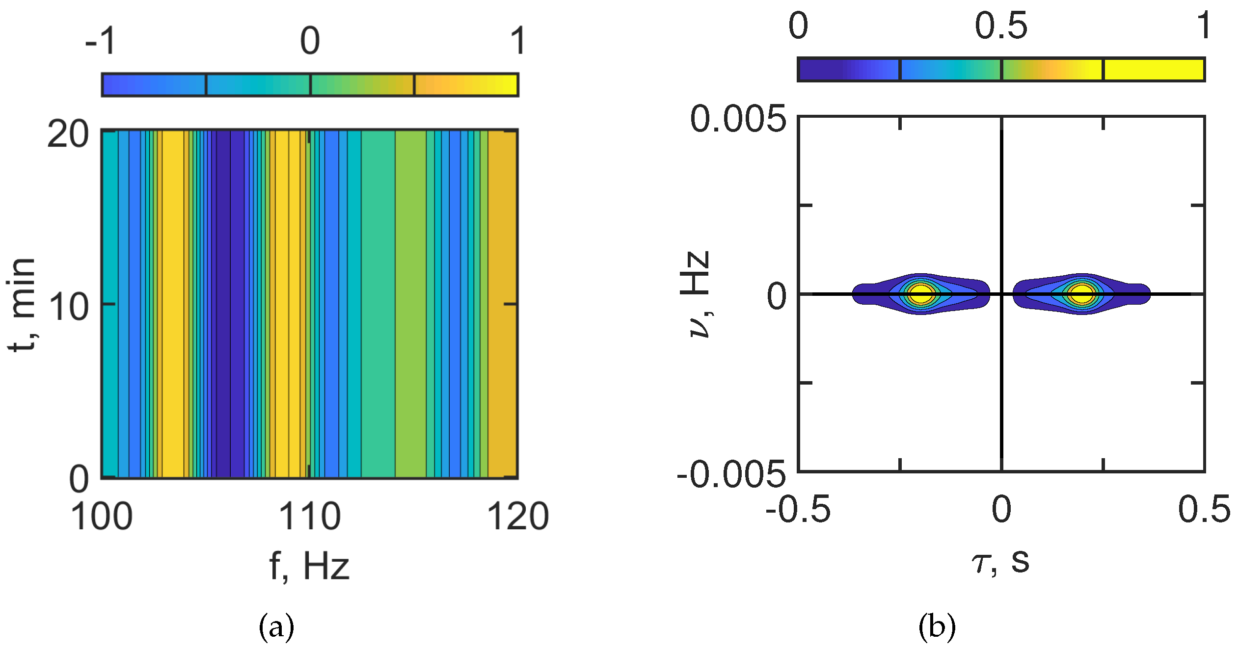
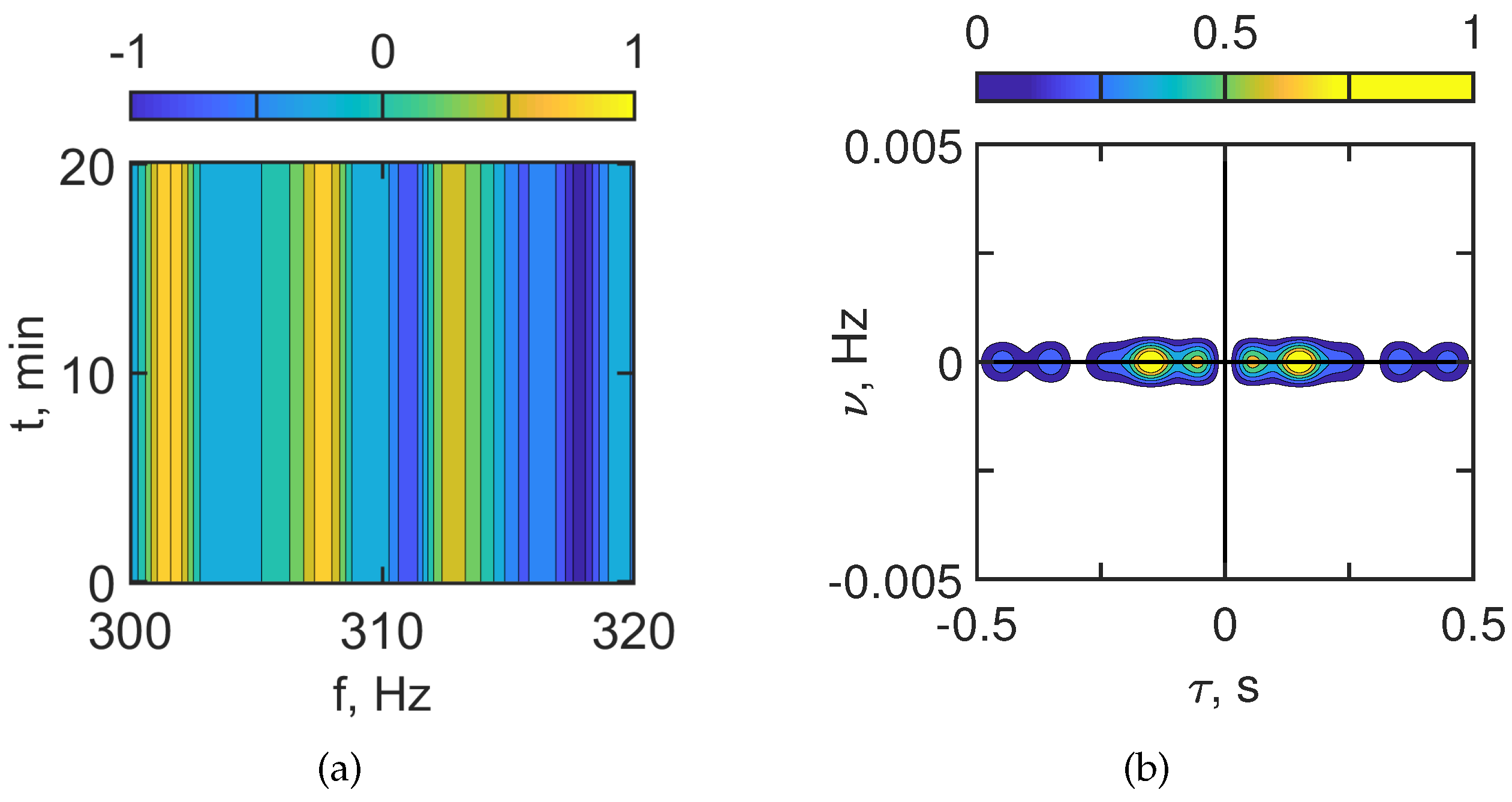
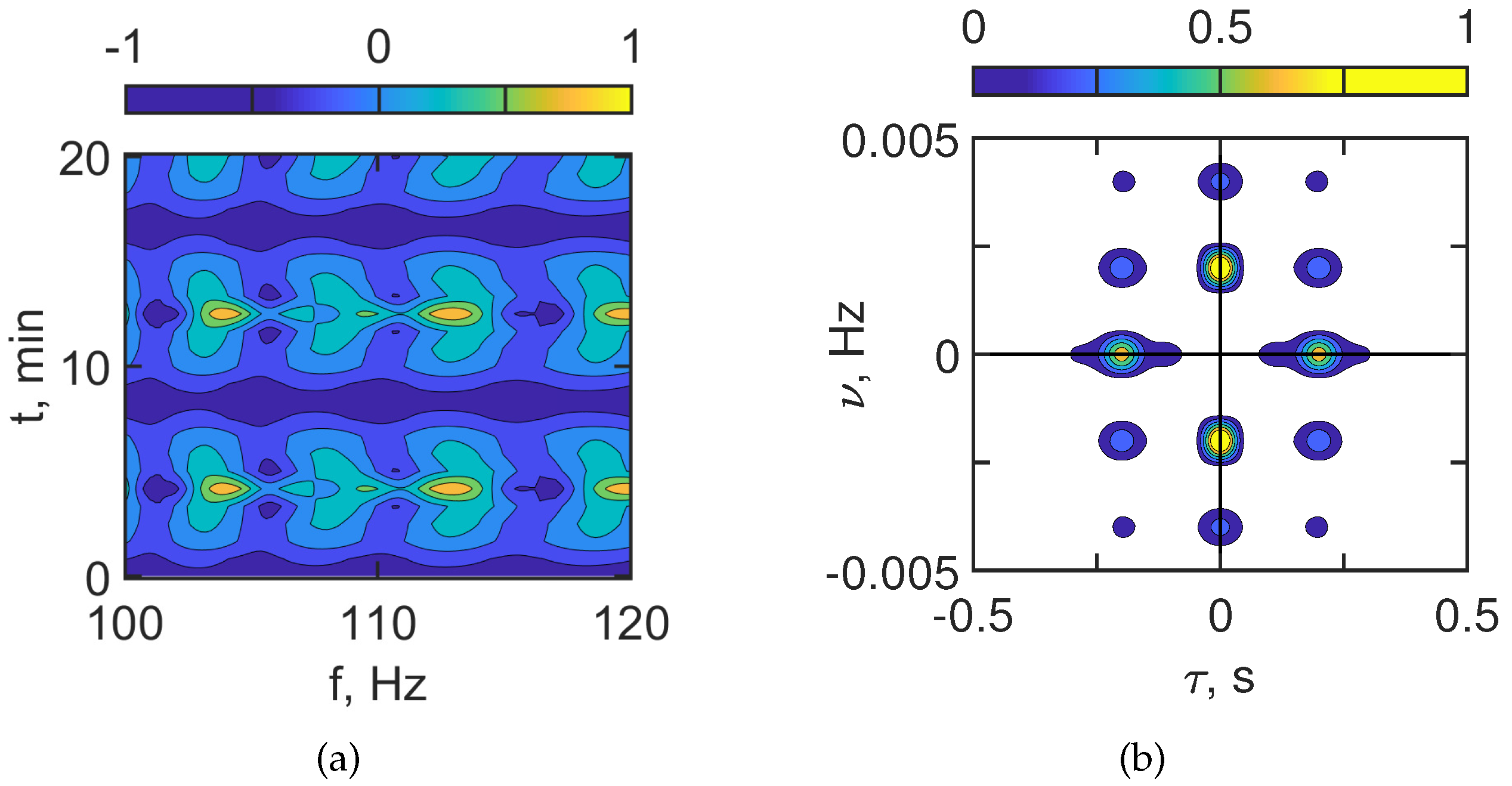
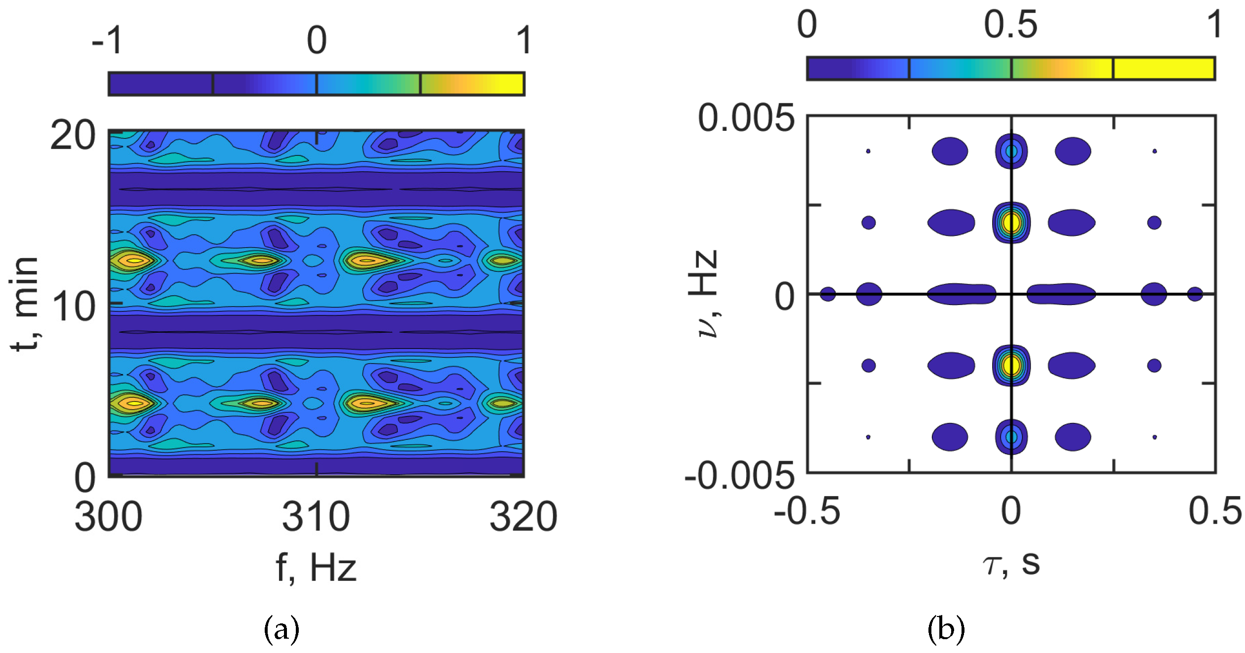
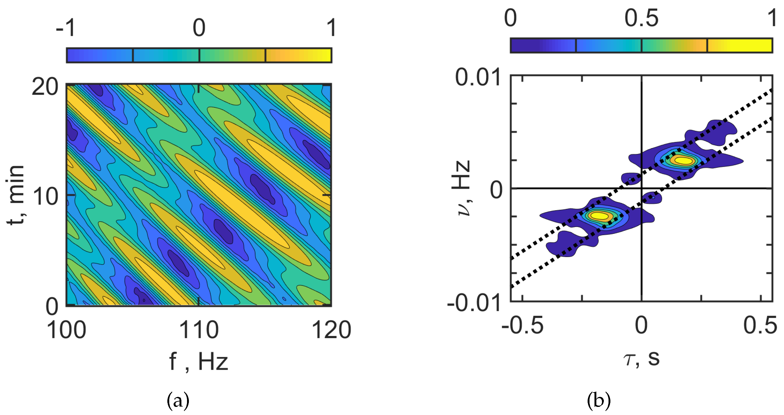
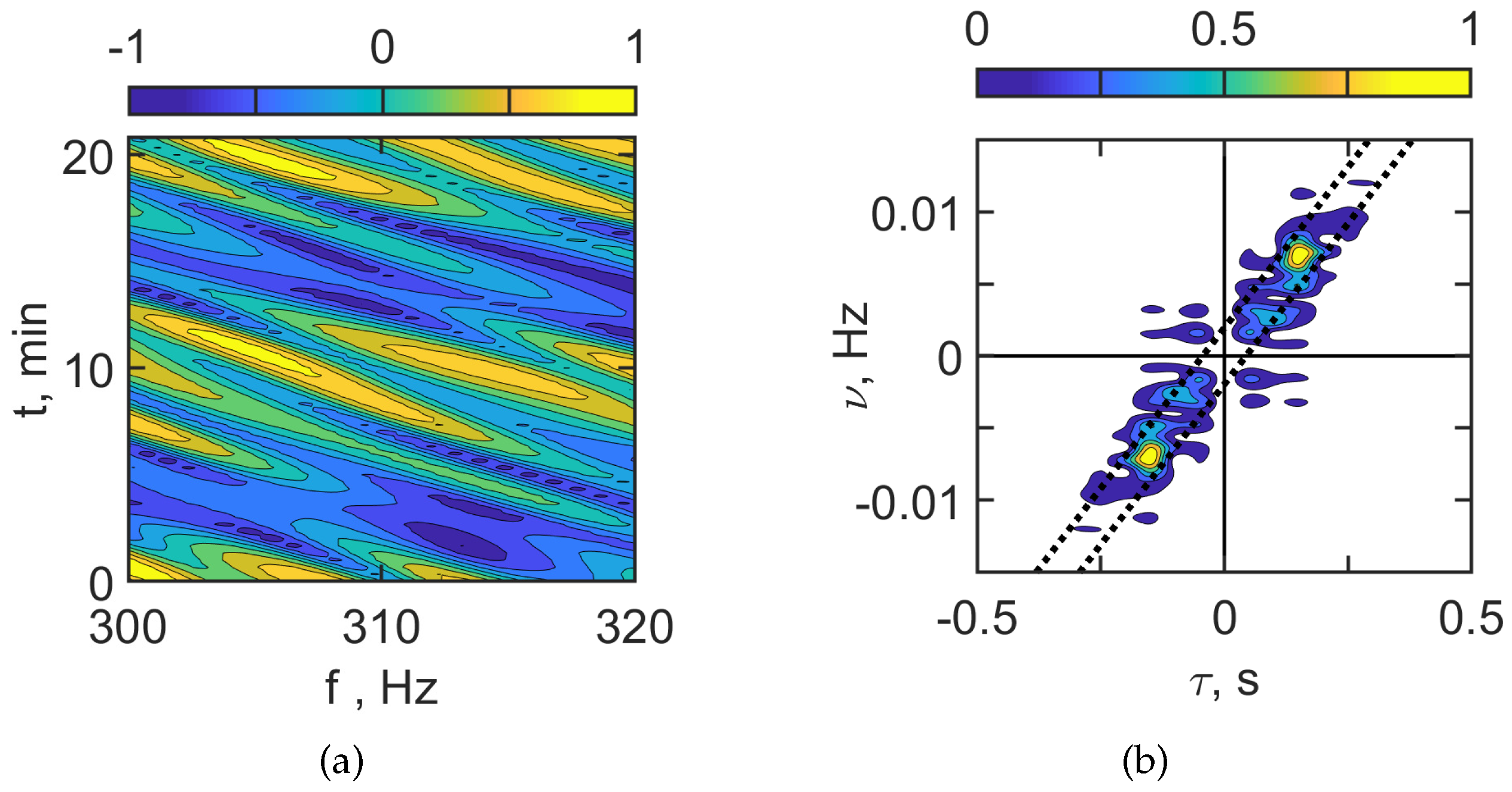
The results of the numerical modeling are shown in Figure 3, Figure 4, Figure 5, Figure 6, Figure 7, Figure 8, Figure 9 and Figure 10. Figure 3 and Figure 4 show the interferogram $I(f,t)$ and the hologram $F(\tau ,\tilde{\nu })$ for the case of the absence of IIWs. Figure 3 corresponds to $\Delta f_1=$ 100–120 Hz and Figure 4 to $\Delta f_2=$ 300–320 Hz. The interferograms $I(f,t)$ consist of localized vertical fringes. The hologram $F(\tau ,\tilde{\nu })$ consists of focal spots on the horizontal axis. This is the result of a non-moving source. The irregularity of the interferogram $I(f,t)$ and the number of focal spots in the hologram $F(\tau ,\tilde{\nu })$ increase with frequency. This is explained by the increase in the number of acoustic modes in the sound field.

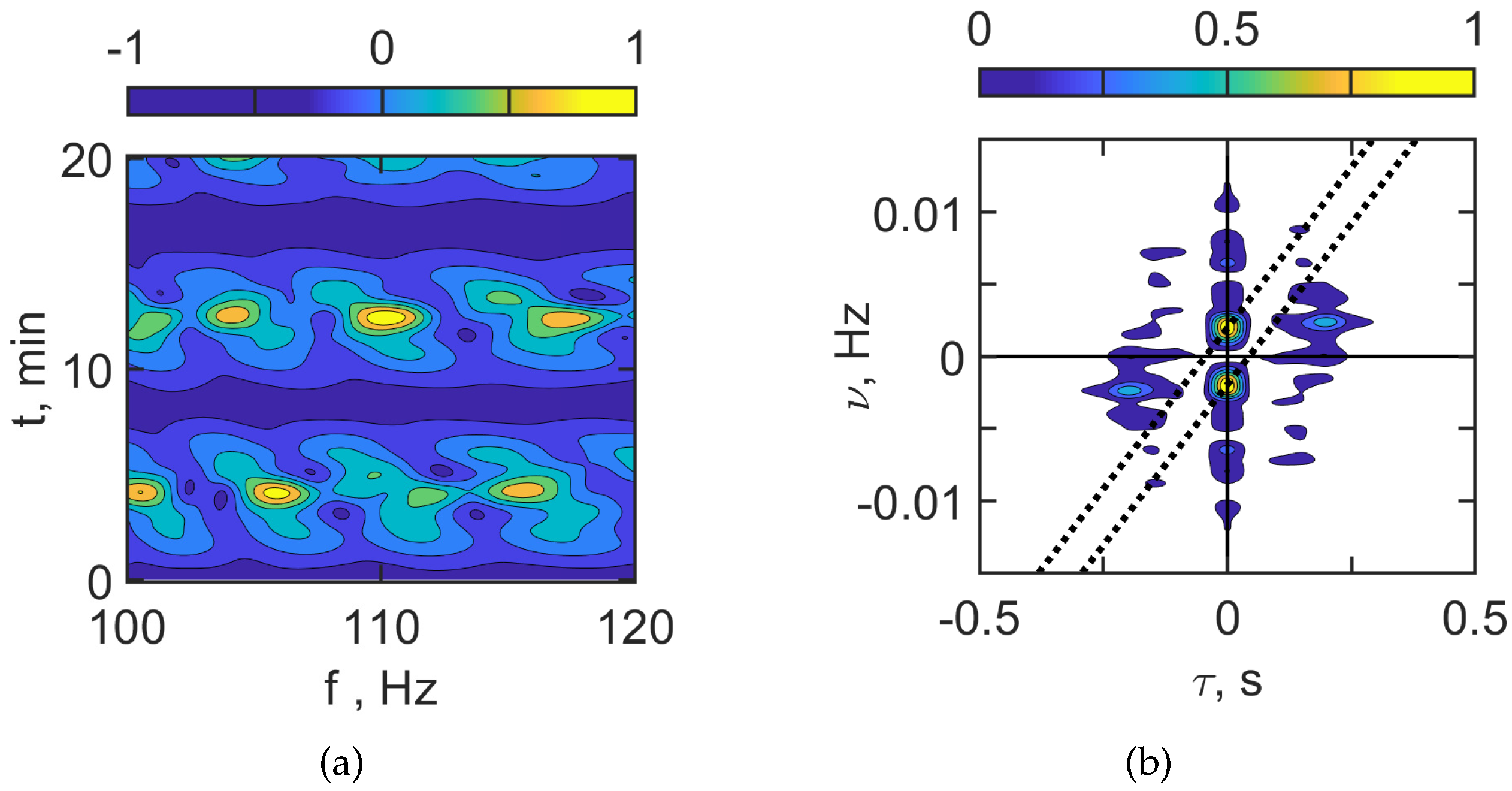
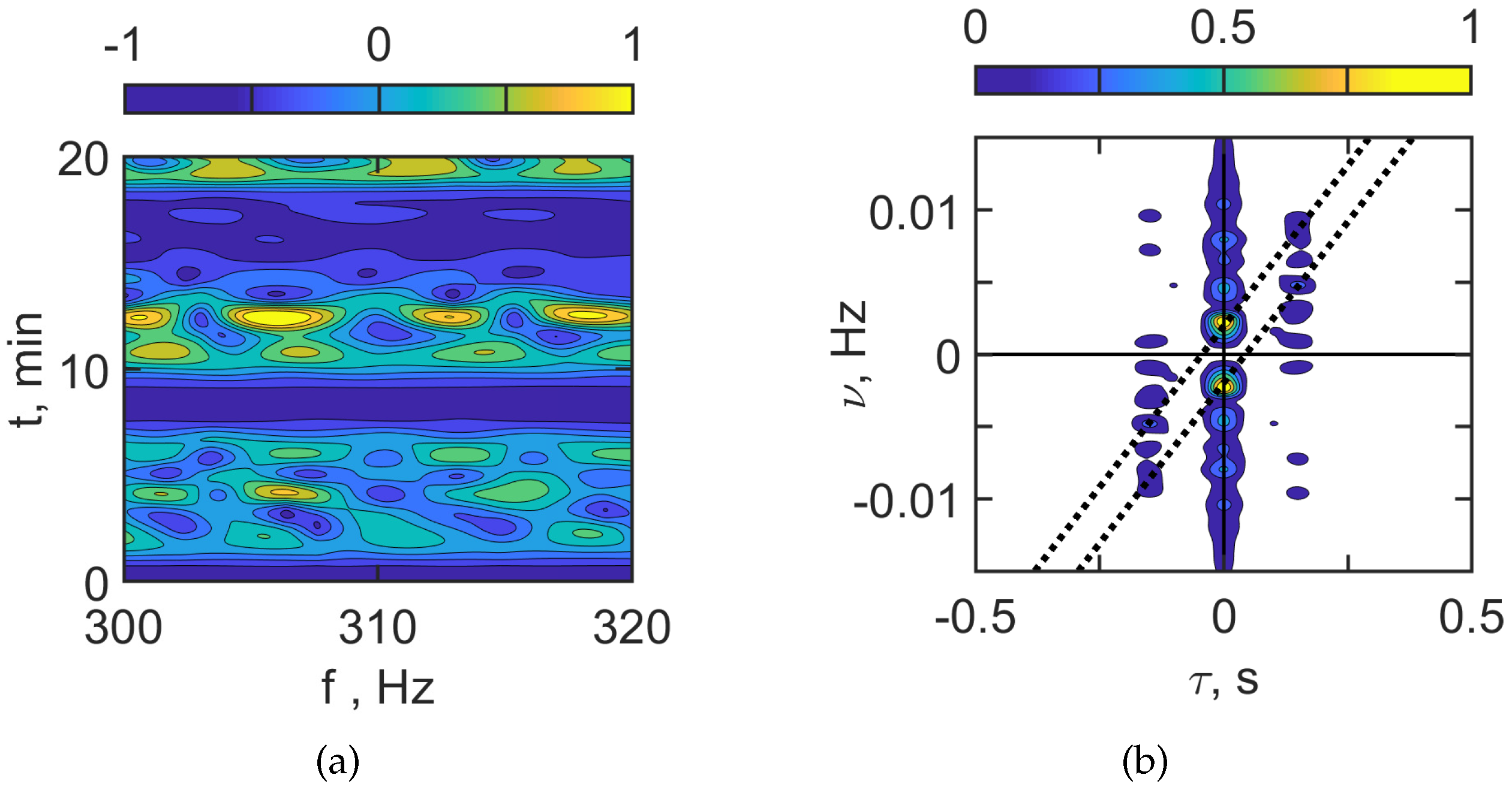
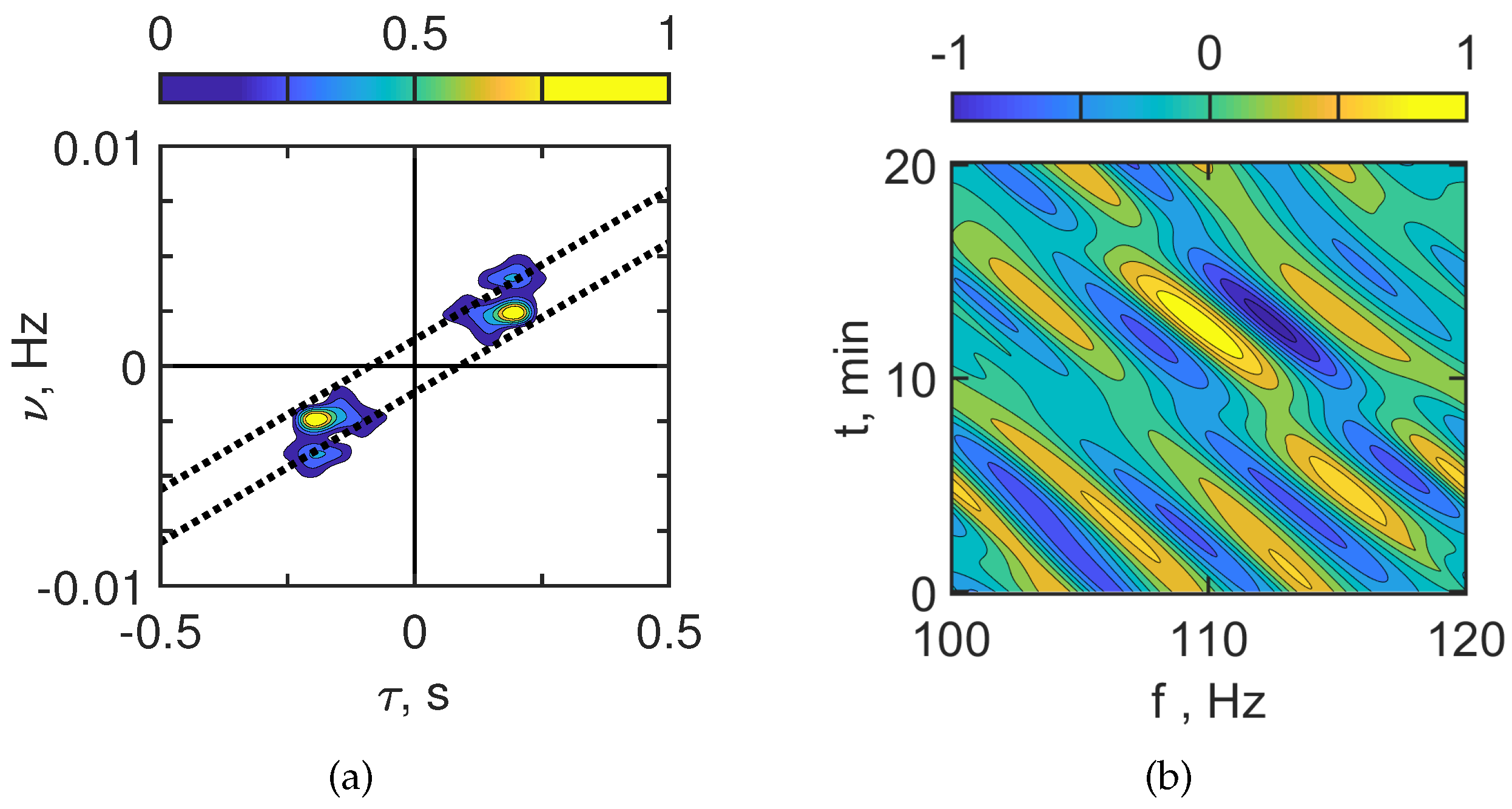
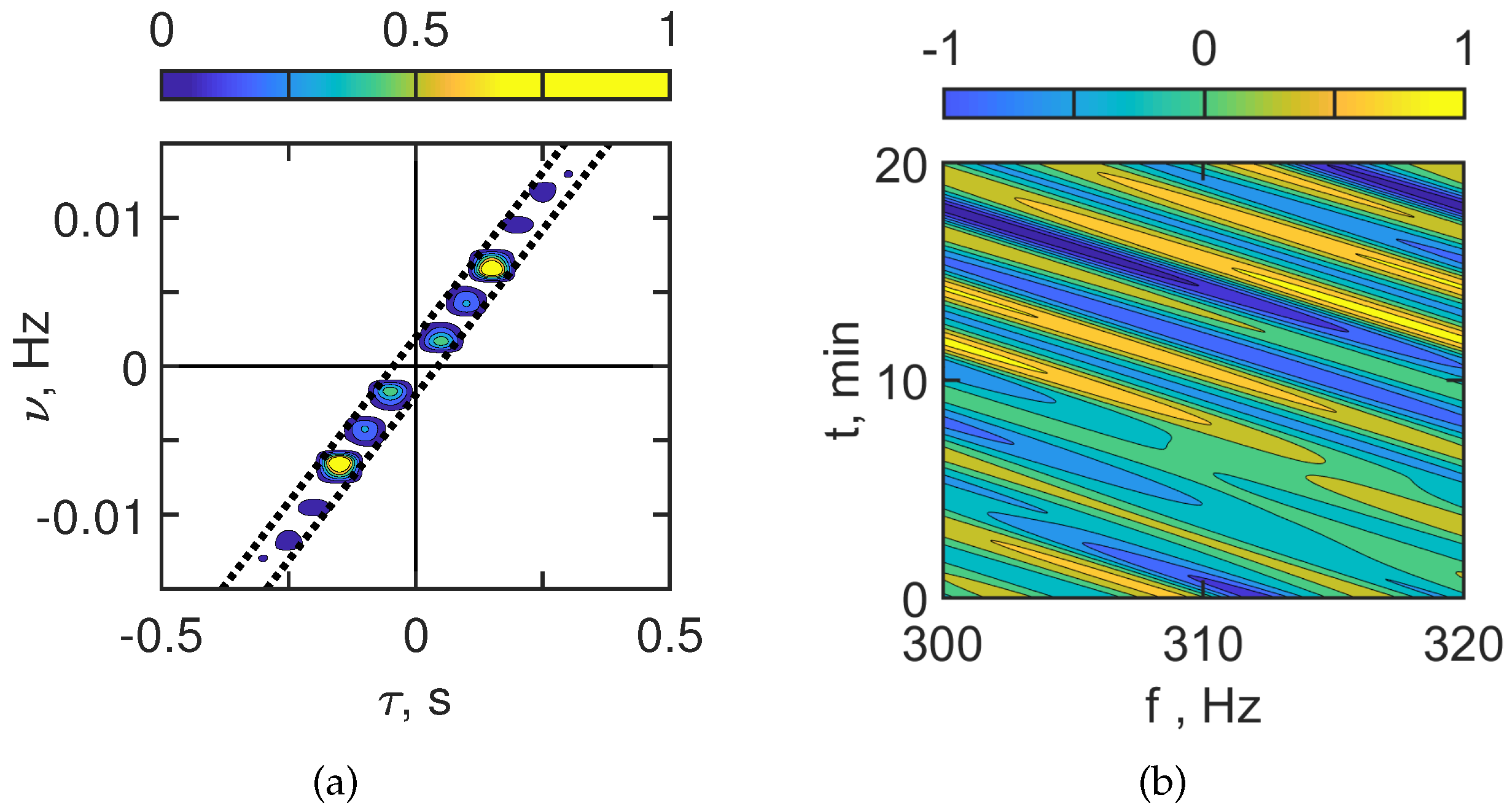
Figure 5 and Figure 6 show the interferogram $I(f,t)$ and the hologram $F(\tau ,\tilde{\nu })$ in the case of the presence of IIWs. Figure 5 corresponds to $\Delta f_1=$ 100–120 Hz and Figure 6 to $\Delta f_2=$ 300–320 Hz. When the acoustic track is located between the IS crests (horizontal spatial period $\mathsf{\Lambda }=250$ m), the interferogram $I(f,t)$ contains horizontal fringes with the width $\Delta t=5.9$ min. In this case, the sound field of the source is focused along the acoustic track due to the horizontal refraction caused by IIWs. Such structure of the interferogram $I(f,t)$ with horizontal fringes leads to the formation of a periodic structure of focal spots in the hologram $F(\tau ,\tilde{\nu })$.

The estimates for the focal spot sizes $\delta f$, $\delta t$, and periodicity intervals $L_f$ and $L_t$ read:

• $\Delta f_1=$ 100–120 Hz;
  $\delta f_1=2.5$ Hz, $\delta t_1=1.3$ min;
  $L_{f_1}=9.2$ Hz, $L_{t_1}=8$ min.
• $\Delta f_2=$ 300–320 Hz;
  $\delta f_2=3.5$ Hz, $\delta t_2=1.3$ min;
  $L_{f_2}=5.5$ Hz, $L_{t_2}=8$ min.

Under natural conditions, the IIW train consists of different ISs with different parameters. This leads to a blurring of the pronounced periodic structure of interferogram $I(f,t)$ and hologram $F(\tau ,\tilde{\nu })$.

The structure of the focal spot arrangement in the hologram $F(\tau ,\tilde{\nu })$ allows for the separation of the component corresponding to the waveguide without IIWs and the sound field component related to the perturbation by IIWs.

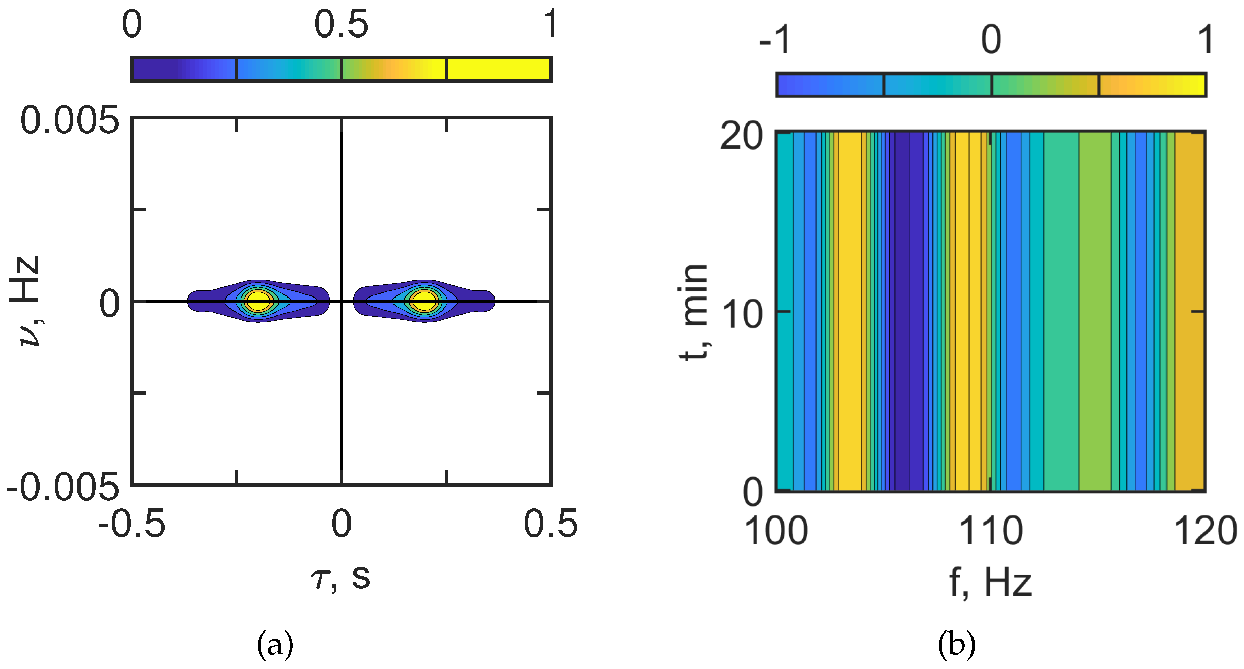
The results of filtering the hologram focal spots located mainly on the horizontal axis in Figure 5 and Figure 6 and their inverse 2D FT (interferogram) are shown in Figure 7 and Figure 9. The reconstructed interferograms and holograms in Figure 7 and Figure 9 correspond to the interferograms and holograms without IIWs in Figure 3 and Figure 4. It can be seen that the focal spots on the reconstructed and the initial hologram are the same. 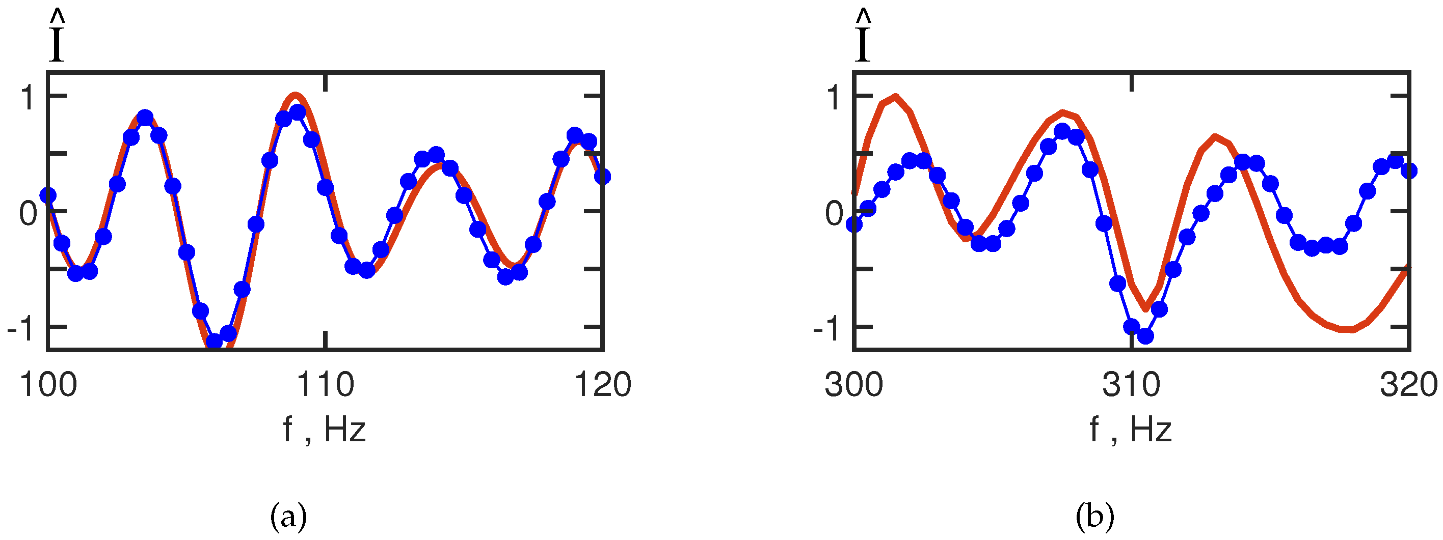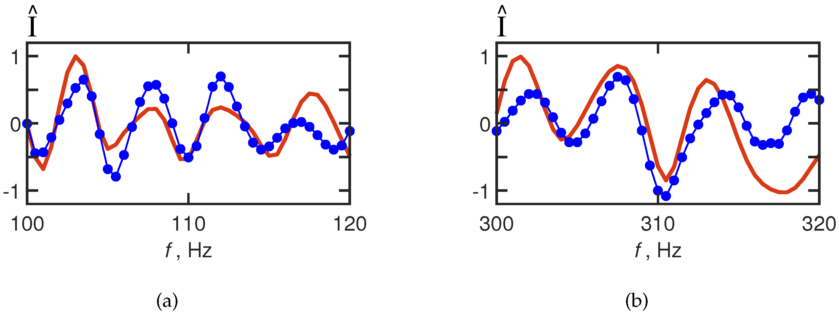The closeness of the initial and reconstructed interferograms is shown in Figure 10. Figure 10 shows the 1D interferograms for $t_0=0$ min. Red curve – IIWs are absent. Blue curve – IIWs are present.

The interferogram reconstruction error is estimated by the dimensionless quantity:

$$d=\frac{{\sum }_{j=1}^J\left|I_1\left(f_j\right)-I_2\left(f_j\right)\right|}{{\sum }_{j=1}^J\left|I_1\left(f_j\right)\right|},$$

(23)

where $I_1\left(f\right)$, $I_2\left(f\right)$ are initial and reconstructed 1D interferograms, respectively.

• $\Delta f_1=$ 100–120 Hz;
  $d_1=0.117$, $J=80$.
• $\Delta f_2=$ 300–320 Hz;
  $d_2=0.096$, $J=80$.

The numerical modeling results for the frequency range $\Delta f_2=$ 300–320 Hz are identical to those for the range $\Delta f_1=$ 100–120 Hz. From the presented results, it follows that the described method allows one to separate the sound field component corresponding to the waveguide without IIWs and the sound field component related to the interference by IIWs. Thus, the interferogram of the waveguide without IIWs can be reconstructed for the case of the non-moving source in the presence of IIWs.

5.3. Moving Source ($v=1$ m/s)

Let us consider the results of numerical modeling for a moving source ($v=1$ m/s). At the initial time $t_0=0$, the source–receiver range is $x_0=10$ km. The source depth is $z_s=20$ m. The receiver depth is $z_q=45$ m. The source moves along the horizontal axis X to the receiver. The velocity of the source is $v=1$ m/s. The source spectrum is uniform. The sound field pulses have duration $t_1=4$ s (sampling frequency $0.25$ Hz). The interval between the end of the previous and the beginning of the next pulse $t_2=1$ s. Therefore, time interval between pulses $t^{*}=5$ s, ($t^{*}=t_1+t_2$). The time observation is $\Delta t=20$ min. The two frequency bands $\Delta f_1=$ 100–120 Hz (Table 1) and $\Delta f_2=$ 300–320 Hz (Table 2) are considered.

The results of the numerical modeling are shown in Figure 11, Figure 12, Figure 13, Figure 14, Figure 15 and Figure 16. The dashed lines on the holograms show the band where the focal spots of the sound field of the moving source are concentrated in the waveguide without IIWs. It can be seen that the linear size of the band: $\delta \tau \approx 0.15$ s, $\delta \nu \approx 0.002$ Hz corresponds to the theoretical estimates of the focal spots sizes $\delta \tau =0.1$ s, $\delta \nu =0.0017$ Hz.

Figure 11 and Figure 12 show the interferogram $I(f,t)$ and the hologram $F(\tau ,\tilde{\nu })$ of the moving source for the case where there are no IIWs. Figure 11 corresponds to $\Delta f_1=$ 100–120 Hz and Figure 12 to $\delta f_2=$ 300–320 Hz. The interferograms $I(f,t)$ consist of localized angled fringes. The hologram $F(\tau ,\tilde{\nu })$ consists of focal spots in the dotted line band. This is the result of the movement of the source. The irregularity of the interferogram $I(f,t)$ and the number of focal spots in the hologram $F(\tau ,\tilde{\nu })$ increase with frequency, as they do for a non-moving source.

The estimates of the interferogram and hologram parameters are as follows:

• $\Delta f_1=$ 100–120 Hz;
  Interference fringes angular coefficients: $\delta f/\delta t\approx -0.015$ s${}^{-2}$;
  First focal spot coordinates ${\tau }_1=1.30·{10}^{-1}$ s, $v_1=1.79·{10}^{-3}$ Hz;
  Source parameters (range and velocity): $\dot{v}=1.0$ m/s, ${\dot{x}}_0=11.8$ km.
• $\Delta f_2=$ 300–320 Hz;
  Interference fringes angular coefficients: $\delta f/\delta t\approx -0.04$ s${}^{-2}$;
  First focal spot coordinates ${\tau }_1=4.08·{10}^{-1}$ s, $v_1=1.54·{10}^{-3}$ Hz;
  Source parameters (range and velocity): $\dot{v}=1.0$ m/s, ${\dot{x}}_0=12.0$ km.

Figure 13 and Figure 14 show the interferogram $I(f,t)$ and the hologram $F(\tau ,\tilde{\nu })$ of the moving source in the case of IIW presence. Figure 13 corresponds to $\Delta f_1=$ 100–120 Hz and Figure 14 to $\Delta f_2$= 300–320 Hz. When the acoustic track is located between the crests of the IS (horizontal spatial period $\mathsf{\Lambda }=250$ m), the interferogram $I(f,t)$ contains horizontal fringes with the width $\Delta t=5.8$ min. In this case, the field of the source is focused along the acoustic track due to the horizontal refraction caused by IIWs. Such a structure of the interferogram $I(f,t)$ with horizontal fringes leads to the formation of a periodic structure of focal spots in the hologram $F(\tau ,\tilde{\nu })$.

The estimates for the focal spots sizes $\delta f$, $\delta t$, and periodicity intervals $L_f$ and $L_t$ read:

• $\Delta f_1=$ 100–120 Hz;
  $\delta f_1=2.4$ Hz, $\delta t_1=1.1$ min;
  $L_{f_1}=5.6$ Hz, $L_{t_1}=8.3$ min.
• $\Delta f_2=$ 300–320 Hz;
  $\delta f_2=2.8$ Hz, $\delta t_2=1.1$ min;
  $L_{f_2}=6.8$ Hz, $L_{t_2}=8.1$ min.

The structure of the arrangement of focal spots in the hologram $F(\tau ,\tilde{\nu })$ of the moving source allows one to separate the sound field component corresponding to the waveguide without IIWs and the sound field component related to the disturbance by IIWs.

The results of the filtration of the hologram focal spots are shown in the dotted lines of Figure 13 and Figure 14, and their inverse 2D FT (interferogram) are shown in Figure 15 and Figure 16. The reconstructed interferograms and holograms in Figure 15 and Figure 16 correspond to the interferograms and holograms without IIWs in Figure 11 and Figure 12. It can be seen that the focal spots on the reconstructed and the initial hologram are close to each other.

The estimates of the filtered interferogram and filtered hologram parameters read:

• $\Delta f_1=$ 100–120 Hz;
  First focal spot coordinates ${\tau }_1=1.5·{10}^{-1}$ s, $v_1=2.05·{10}^{-3}$ Hz;
  Source parameters (range and velocity): $\dot{v}=1.2$ m/s, ${\dot{x}}_0=13.7$ km.
• $\Delta f_2=$ 300–320 Hz;
  First focal spot coordinates ${\tau }_1=4.08·{10}^{-1}$ s, $v_1=1.54·{10}^{-3}$ Hz;
  Source parameters (range and velocity): $\dot{v}=1.0$ m/s, ${\dot{x}}_0=12.0$ km.

It can be seen that the focal spots on the reconstructed and initial holograms of the moving source are the same. The proximity of the initial and reconstructed interferograms of the moving source is shown in Figure 16. Figure 16 shows the 1D interferograms for $t_0=0$ min. Red curve –IIWs are not present. Blue curve – IIWs are present.

The error of the interferogram reconstruction is estimated by the dimensionless quantity Equation (23):

• $\Delta f_1=$ 100–120 Hz;
  $d_1=0.45$, $J=80$.
• $\Delta f_2=$ 300–320 Hz;
  $d_2=0.60$, $J=80$.

Compared to the non-moving source, the error for the frequency ranges $\Delta f_1=$ 100–120 Hz and $\Delta f_2=$ 300–320 Hz has increased by a factor of $3.7$ and $6.2$, respectively. It can be seen that the interferogram of the waveguide without IIWs is reconstructed less accurately for a moving source. This difference in the error values is due to difference in variation of the propagation conditions. In the case of the non-moving source, there is waveguide variability due to IIWs only. In the case of the moving source, there is waveguide variability due to IIWs and due to movement of the source.

6. Conclusions

The stability of the HSP method in the case of the moving broadband acoustic source source in presence of IIWs is analyzed. IIWs are assumed to propagate across the acoustic track (source–receiver). In this case, IIWs cause significant horizontal refraction of the sound field. As a result, the dynamic horizontal waveguides are approximately parallel to the IIW fronts in the horizontal plane.

The sound intensity is periodically focused and defocused along the IIW front direction. This results in significant variations in sound intensity (∼4–5 dB) at the receiver point. However, HSP allows the received signal in shallow water waveguides to be freed from such a significant obstacle caused by IIWs. The stability of HSP is based on the hologram structure of the moving source in presence of IIWs. The hologram of the moving source consists of two disjoint components. The first is the sound field component corresponding to the waveguide without IIWs. The second component is the perturbation of the field by the IIWs causing horizontal refraction. Such a hologram structure allows the separation of the sound field components. It is possible to filter the first component with minimal distortion. The filtered hologram component is used to reconstruct the interferogram of a moving source in waveguide in absence of IIWs. The reconstructed sound field interferograms in presence of IIWs and interferograms in waveguide without IIWs differ in contrast.

The interferogram reconstruction error is $d_1=0.117$ ($\Delta f_1=$ 100–120 Hz), $d_2=0.096$ ($\Delta f_2=$ 300–320 Hz) for the non-moving source and $d_1=0.45$ ($\Delta f_1=$ 100–120 Hz), $d_2=0.60$ ($\Delta f_2=$ 300–320 Hz) for the moving source. However, the angular coefficients of interferogram fringes are the same.

Thus, in presence of IIWs, it is possible to estimate the parameters of the source (range, velocity, direction, etc.) from the reconstructed sound field component. The error in estimating the source parameters decreases with an increase of frequency.