Bottom Multi-Parameter Bayesian Inversion Based on an Acoustic Backscattering Model

Abstract

The geoacoustic and physical properties of the bottom, as well as spatial distribution, are crucial factors in analyzing the underwater acoustic field structure and establishing a geoacoustic model. Acoustic inversion has been widely used as an economical and effective method to obtain multi-parameters of the bottom. Compared with traditional inversion methods based on acoustic propagation models, acoustic backscattering models are more suitable for multi-parameter inversion, because they contain more bottom information. In this study, a Bayesian inversion method based on an acoustic backscattering model is proposed to obtain bottom multi-parameters, including geoacoustic parameters (the sound speed and loss parameter), partial physical parameters of the sediment, and statistical parameters of the seafloor roughness and sediment heterogeneity. The bottom was viewed as a kind of fluid medium. A high-frequency backscattering model based on fluid theory was adopted as the forward model to fit the scattering strength between the model prediction and the measured data. The Bayesian inversion method was used to obtain the posterior probability density (PPD) of the inversion parameters. Parameter estimation, uncertainty, and correlation were acquired by calculating the maximum a posterior (MAP), the mean values, the one-dimensional marginal distributions of the PPD, and the covariance matrix. Finally, the high-frequency bottom backscattering strength from the Quinault Range site was employed for inversion tests. The estimated values and uncertainties of various bottom parameters are presented and compared with the directly measured bottom parameters. The comparison results demonstrate that the method proposed herein can be used to estimate the sediment/water sound speed ratio, the sediment/water density ratio, and the spectral exponent of the roughness spectrum effectively and reliably.

1. Introduction

Bottom characteristic parameters play an important role in theoretical modeling of the acoustic field and the evaluation of sonar system performance [1,2]. Therefore, the accurate acquisition of bottom characteristic parameters has always been a popular topic in the field of marine acoustics [3]. Traditional methods for acquiring bottom parameters include in situ measurements and sampling measurements, which are not only technically challenging but also unsuitable for obtaining large-scale bottom parameters [2,4,5]. Acoustic inversion, in contrast to direct measurement methods, offers a more cost-effective approach to acquiring bottom parameters [6,7].

Acoustic inversion is actually a multidimensional optimization problem that can be divided into four steps: 1. selecting an appropriate objective function to accurately represent the degree of match between the actual observational data and the synthetic data; 2. devising an appropriate forward model for calculating the synthetic data; 3. implementing a highly efficient global optimization algorithm to search for the optimal values of each inversion parameter; and 4. performing an uncertainty analysis of the inversion results [8]. Among these steps, the selection of the forward model is an important prerequisite for inversion. In most studies on acoustic inversion, underwater acoustic propagation models are typically used as the forward model [8,9]; the matching physical quantities used for inversion include normal mode dispersion characteristics, the bottom reflection coefficient, sound propagation loss, and so on [10,11,12]. Under this condition, the parameters obtained via acoustic inversion are usually sediment acoustic parameters (sound speed and attenuation coefficient), sediment density, and the layered structure. However, these parameters do not fully meet the requirements of theoretical studies, such as explaining the complex acoustic mechanisms of the bottom. For example, acoustic scattering modeling requires parameters that are used to characterize seafloor roughness and sediment heterogeneity [13,14]. Bottom acoustic scattering is related to the rough water–sediment interface and the sediment heterogeneity. Therefore, the received scattering data interacting with the bottom will contain more information about the bottom. This provides a new idea for bottom multiparameter inversion [15]. Turgut [16] utilized acoustic backscattering data to efficiently extract additional bottom statistical parameters through an inversion method for various sediment types. The obtained parameters included acoustic parameters, physical parameters, and statistical parameters of seafloor roughness and sediment heterogeneity. Zou et al. and Yu et al. [17,18] obtained similar results by using acoustic scattering models. However, the difference between these methods is that, in the former, acoustic scattering models with different geoacoustic models were used for inversion, whereas in the latter, the bottom was regarded as a poroelastic medium, and acoustic scattering models based on the equivalent density fluid approximation were used for inversion. The aforementioned studies demonstrate that the acoustic scattering model can be utilized as the forward model for acoustic inversion to obtain additional bottom parameters.

Acoustic inversion is a nonlinear problem with multiple solutions [19]. The more unknown parameters there are to be inverted, the more complex the problem will be. In addition, the complex ocean environment introduces systematic and random errors in the measured data and theoretical errors in the forward model [20]. These factors will impact the accuracy of the inversion results. Therefore, conducting an uncertainty analysis of the inversion results is crucial [21]. To quantify the uncertainty of the inversion results, the Bayesian method is widely used in parameter inversion [22,23]. Bayesian inversion theory combines prior information from the forward model with observed data to analyze the posterior probability density (PPD) of the inversion results using statistical theory [24]. The uncertainty analysis is conducted by sampling the model parameters, and the MAP estimation of the parameters is obtained through numerical integration [22].

In this paper, we propose a Bayesian inversion method based on an acoustic backscattering model to obtain bottom multi-parameter and analyze the uncertainties and correlations of inversion results. The following assumptions are made in the inversion: 1. the seabed is modeled as a half-space with a rough interface at the seafloor and volume inhomogeneities within the half-space; and 2. the sediment is treated as a fluid medium. Comparing with traditional inversion methods on the basis of acoustic propagation, we employ a simpler theoretical model and obtain more bottom information in this study (e.g., geoacoustic parameters and sediment density, as well as parameters associated with the seafloor roughness and sediment volume scattering). In the inversion process, the backscattering strength is considered the matching physical quantity of the inversion problem. The marginal PPD of the inversion parameters is then obtained according to the Bayesian inversion method to analyze the uncertainties and correlations of the inversion results. Compared with the available methods based on the acoustic scattering model, we ignore the poroelasticity of the sediment to reduce the inversion parameters by treating the bottom as a fluid medium, focusing on inversion of the key parameters (the sediment/water speed ratio, sediment/water density ratio, and loss parameter). Furthermore, an empirical parameter (the volume scattering cross section/attenuation coefficient ratio) is employed to characterize the volume scattering resulting from its lesser contribution to the overall backscattering strength in sandy sediment [25]. The purpose is to decrease the inversion uncertainty caused by weakly sensitive or insensitive parameters used to characterize volume scattering.

The remainder of this paper is organized as follows. In Section 2, the backscattering model based on fluid theory is simply introduced. The Bayesian inversion method is presented in Section 3. In Section 4, a numerical simulation is demonstrated to test the feasibility of the proposed inversion method in this study. Section 5 utilizes the measured backscattering strength at 35 kHz from the Quinault Range site to validate the inversion method, including a comparison between the inversion and measurement results of the bottom parameters and uncertainty analysis. The conclusion is provided in Section 6.

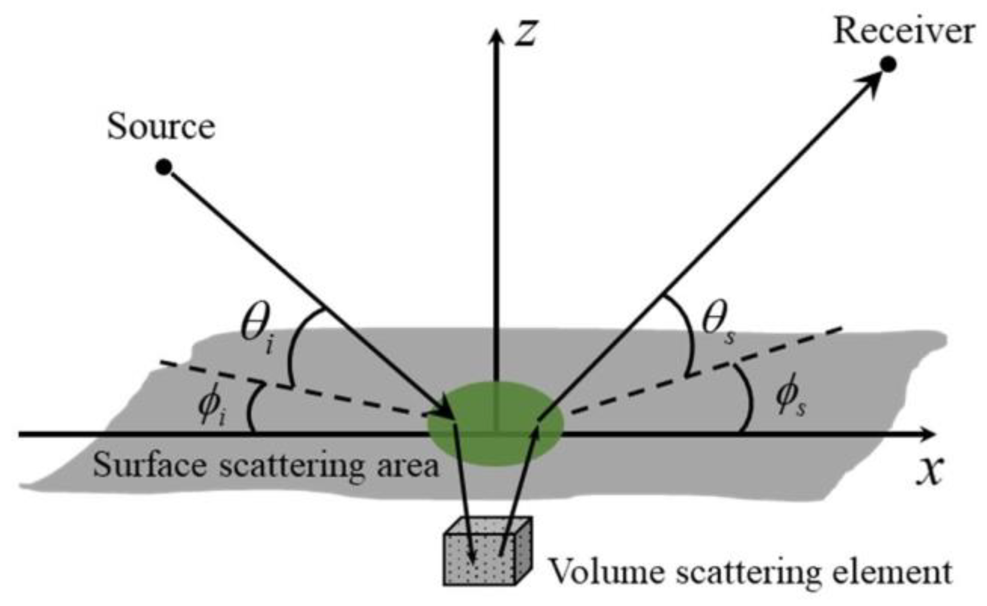
2. Acoustic Backscattering Model

We adopted the acoustic backscattering model derived by Jackson and Richardson [1] as the forward model, because it is suitable for high frequencies (10–100 kHz). Figure 1 shows the definitions of the angles used in treating scattering. The parameters ${\theta }_i$ and ${\theta }_s$ represent the grazing angles of the incident and scattered waves, respectively. The parameters ${\varphi }_i$ and ${\varphi }_s$ represent the azimuthal angles of the incident and scattered waves, respectively. Without the loss of generality, we assume that ${\varphi }_i=0°$. For bottom backscattering, ${\theta }_i={\theta }_s=\theta$ and ${\varphi }_s=180°$. The backscattering strength is a physical quantity used to characterize the backscattering ability of the bottom and was therefore chosen as the matching physical quantity for the inversion problem. It is attributed to the seafloor roughness and the sediment heterogeneity. The backscattering strength $S_b$ can be described as the following function of grazing angle $\theta$ and incident frequency $f$ [1,26,27]:

$$S_b\left(\theta ,f\right)=10{\log }_{10}\left[{\sigma }_{br}\left(\theta ,f\right)+{\sigma }_{bv}\left(\theta ,f\right)\right],$$

(1)

where ${\sigma }_{br} (\theta ,f)$ is the roughness scattering cross-section and ${\sigma }_{bv} (\theta ,f)$ is the equivalent interface scattering cross-section. Below the mid-grazing angle $(<70°)$, the roughness scattering cross-section can be calculated using the small-roughness perturbation approximation based on the fluid sediment model [28]. The fluid sediment model was also employed to handle scattering caused by sediment heterogeneity.

2.1. Roughness Scattering Model

Seafloor roughness is a main factor that influences high-frequency acoustic scattering. To characterize the statistical properties of the seafloor roughness within a limited scale range, it can be assumed that it follows an isotropic two-dimensional (2D) spectrum subjected to a power-law function of the wave number [29]:

$$W\left(K\right)=\frac{w_2}{{\left(h_{0}K\right)}^{{\gamma }_2}},$$

(2)

where $K$ is the magnitude of the 2D wave vector, $h_0$ is the reference length ($h_0=1$ cm), and $w_2$ and ${\gamma }_2$ represent the spectral strength and the spectral exponent of the roughness spectrum, respectively. The range of values for ${\gamma }_2$ is

$$2\le {\gamma }_2\le 4.$$

(3)

Based on the roughness spectrum, researchers have developed the following small-roughness perturbation approximation equation that is formally independent of the specific wave theory (i.e., the medium type):

$${\sigma }_{br}=k_w^4{\left|A_{ww}\right|}^{2}W\left(\Delta \mathbf{K}\right),$$

(4)

where $k_w$ is the wave number in water, $A_{ww}$ is the small-roughness perturbation approximation factor (which depends on different wave theories), and $\mathsf{\Delta }\mathbf{K}$ is the Bragg wave vector [30].

Under the fluid sediment model assumption, Jackson et al. [26] provided a straightforward approach to solve for the variable $A_{ww}$ in Equation (4) when applied to isotropic sediments:

$$A_{ww}=\frac{1}{2}{\left[1+V_{ww}\left(\theta \right)\right]}^{2}G,$$

(5)

where

$$G=\left(1-\frac{1}{{\rho }_b}\right)\left[{\cos }^2\theta -\frac{{\sin }^2{\theta }_{pi}}{a_p^2{\rho }_b}\right]-1+\frac{1}{a_p^2{\rho }_b},$$

(6)

with

$${\sin }^2{\theta }_{pi}=\sqrt{1-a_p^2{\cos }^2\theta },$$

(7)

and where $V_{ww} \left(\theta \right)$ is the reflection coefficient of a flat interface at grazing angle $\theta$, ${\rho }_b$ is the sediment/water density ratio, and $a_p$ is the sediment/water complex sound speed ratio. $a_p$ is given by

$$a_p=\frac{v_b}{1+i{\delta }_b},$$

(8)

where $v_b (v_b=c_s/c_w)$ is the real sediment/water speed ratio (where $c_s$ and $c_w$ denote the sediment and water sound speed, respectively), and ${\delta }_b$ is the loss parameter (dimensionless) of the sediment. The relationship between the loss parameter ${\delta }_b$ and the attenuation coefficient ${\alpha }_p$ is as follows:

$${\delta }_b=\frac{{\alpha }_p{v}_b{c}_w\ln \left(10\right)}{40\pi f}.$$

(9)

2.2. Volume Scattering Model

Volume scattering at high frequencies can be treated experimentally and theoretically as an interfacial process. Jackson et al. [26] provided the following formula for calculating the equivalent interface scattering cross-section:

$${\sigma }_{bv}=\frac{{\sigma }_v{\left|1-V_{ww}{\left(\theta \right)}^2\right|}^2{\sin }^2\theta }{4k_w{\left|P\left(\theta \right)\right|}^2\mathrm{Im}\left[P\left(\theta \right)\right]},$$

(10)

where

$$P\left(\theta \right)=\sqrt{{\left(1/a_p\right)}^2-{\cos }^2\theta },$$

(11)

and ${\sigma }_v$ is the volume scattering cross-section. Similar to the seafloor roughness spectrum mentioned in Section 2.1, there is a corresponding power-law spectrum for volume scattering to characterize the sediment heterogeneity. However, we adopted a relatively simple approach to estimate it. We treated it as a quantity that can be obtained through data fitting, rather than through a theory-based calculation [13]. Under this condition, ${\sigma }_v$ can be expressed as follows:

$${\sigma }_v={\alpha }_p{\sigma }_2,$$

(12)

where ${\sigma }_2$ is a dimensionless variable with a typical value range of 0.0001–0.004. For water-saturated sandy sediments, roughness scattering is dominant compared to volume scattering, while the contribution of the volume scattering strength to the total backscattering strength is weak. Consequently, it is appropriate to use an empirical approach rather than a theoretical one to obtain ${\sigma }_v$. Therefore, ${\sigma }_2$ was chosen to characterize the volume scattering.

3. Inversion Theory

3.1. Bayesian Inversion Theory

In Bayesian inversion theory, PPD is used to describe the solution of an inversion problem. Let $\mathbf{m}$ denote the data vector of bottom parameters and let $\mathbf{d}$ denote the measured data vector. According to the Bayesian rule,

$$P\left(\mathbf{m}\left|\mathbf{d}\right.\right)=P\left(\mathbf{d}\left|\mathbf{m}\right.\right)P\left(\mathbf{m}\right)/P\left(\mathbf{d}\right),$$

(13)

where $P\left(\mathbf{m}\right|\mathbf{d})$ is the PPD, $P\left(\mathbf{d}\right|\mathbf{m})$ is the conditional PPD of the measured data $\mathbf{d}$ under the bottom parameters vector $\mathbf{m}$, and $P\left(\mathbf{d}\right)$ can be regarded as a constant that is independent of inversion. Then Equation (13) can be written as

$$P\left(\mathbf{m}\left|\mathbf{d}\right.\right)\propto P\left(\mathbf{d}\left|\mathbf{m}\right.\right)P\left(\mathbf{m}\right).$$

(14)

In Bayesian theory, $P\left(\mathbf{d}\right|\mathbf{m})$ is defined as the likelihood function of parameters vector $\mathbf{m}$ and is determined by the form of the data and the statistical distribution of data errors [31]. However, in actual applications, it is difficult to independently obtain the statistical characteristics of the errors. In general, one assumes that the data error follows a Gaussian distribution. Then, the likelihood function $L\left(\mathbf{m}\right)$ can be expressed as

$$L\left(\mathbf{m}\right)\propto \exp \left[-E\left(\mathbf{m}\right)\right],$$

(15)

where $E\left(\mathbf{m}\right)$ represents the error function between the measured data and the synthetic data provided by the forward model under the given parameters vector $\mathbf{m}$. Equation (14) can be rewritten as

$$P\left(\mathbf{m}\left|\mathbf{d}\right.\right)\propto \exp \left[-E\left(\mathbf{m}\right)\right]P\left(\mathbf{m}\right),$$

(16)

and is normalized as follows:

$$P\left(\mathbf{m}\left|\mathbf{d}\right.\right)=\frac{\exp \left[-E\left(\mathbf{m}\right)\right]P\left(\mathbf{m}\right)}{{\displaystyle \underset{D}{\int }\exp \left[-E\left({\mathbf{m}}^{\prime }\right)\right]P\left({\mathbf{m}}^{\prime }\right)d{\mathbf{m}}^{\prime }}},$$

(17)

where $D$ represents the integration spans in a multidimensional parameter space.

When applying Bayesian theory to solve multidimensional problems, it is essential to estimate parameter values, uncertainties, and correlations between parameters. These estimates are typically represented by the maximum posteriori probability, mean value, parameter covariance matrix, and marginal probability density $P\left({\mathbf{m}}_i\right|\mathbf{d})$ of the ith parameter, which are denoted, respectively, as

$$\hat{\mathbf{m}}=Ar{g}_{\max }\left(P\left(\mathbf{m}\left|\mathbf{d}\right.\right)\right),$$

(18)

$$\overline{\mathbf{m}}={\displaystyle \int {\mathbf{m}}^{\prime }P}\left({\mathbf{m}}^{\prime }\left|\mathbf{d}\right.\right)d{\mathbf{m}}^{\prime },$$

(19)

$${\mathbf{C}}_{\mathbf{m}}={{\displaystyle \int \left({\mathbf{m}}^{\prime }-\overline{\mathbf{m}}\right)\left(\mathbf{m}\prime -\overline{\mathbf{m}}\right)}}^{T}P\left({\mathbf{m}}^{\prime }\left|{\mathbf{d}}^{\mathbf{o}}\right.\right)d{\mathbf{m}}^{\prime },$$

(20)

$$P({\mathbf{m}}_i\left|\mathbf{d}\right.)={\displaystyle \int \delta \left({\mathbf{m}}_i-{{\mathbf{m}}_i}^{\prime }\right)P\left({\mathbf{m}}^{\prime }\left|\mathbf{d}\right.\right)d{\mathbf{m}}^{\prime }},$$

(21)

where $\delta$ represents the Dirac function.

The correlation between parameters $i$ and $j$, $R_{ij}$, can be described by a normalized covariance matrix $C_m$:

$$R_{ij}=\frac{C_{m_{ij}}}{{\left[C_{m_{ij}}{C}_{m_{ji}}\right]}^{1/2}}.$$

(22)

$R_{ij}$ represents the correlation coefficient, with a value ranging from −1 to 1. $R_{ij}=1$ indicates a strong positive correlation between parameters i and j, while $R_{ij}=-1$ indicates a strong negative correlation, and $R_{ij}=0$ indicates no correlation [18,19]. Furthermore, the correlation between parameters can also be qualitatively analyzed based on the 2D marginal PPDs of the parameter pairs.

3.2. Objective Function and Sampling Method

As mentioned in Section 3.1, it is difficult to independently acquire the statistical characteristics of data errors in practical applications, as it requires making physical assumptions about the uncertainty distribution. By assuming that the data errors follow a Gaussian distribution with a mean value of zero and a covariance matrix of $C_f$ and that the backscattering strength data at different frequencies and grazing angles are uncorrelated, the likelihood function can be written as

$$L\left(\mathbf{m}\right)={\displaystyle \prod _{f=1}^F\frac{1}{{\pi }^N\left|C_f\right|}\exp \left[-{\left[P_{obs}^f-P_{replica}^f\left(\mathbf{m}\right)\right]}^T{C}_f^{-1}\left[P_{obs}^f-P_{replica}^f\left(\mathbf{m}\right)\right]\right]},$$

(23)

where $N$ represents the number of data points corresponding to different grazing angles at a certain frequency, $P_{obs}^f$ denotes the measured backscattering strength data at a certain frequency, and $P_{replica}^f\left(\mathbf{m}\right)$ stands for the synthetic data calculated according to the forward model at a certain frequency for different grazing angles when the parameters vector m is given. By ignoring the spatial correlation of the data, $C_f$ can be rewritten as

$$C_f=v_f\mathbf{I},$$

(24)

where $v_f$ represents the unknown variance at a certain frequency and $\mathbf{I}$ is the identity matrix. The likelihood function can be simplified as

$$L\left(\mathbf{m}\right)={\displaystyle \prod _{f=1}^F\frac{1}{{\left(\pi v_f\right)}^N}\exp \left[-B_f\left(\mathbf{m}\right){\left|P_{obs}^f\right|}^2/v_f\right]},$$

(25)

where $B_f$ is the Bartlett processor, the expression for which is

$$B_f\left(\mathbf{m}\right)=1-\frac{\left|P_{replica}^f{\left(\mathbf{m}\right)}^{†}{P}_{obs}^f\right|}{{\left|P_{replica}^f\left(\mathbf{m}\right)\right|}^2{\left|P_{obs}^f\right|}^2},$$

(26)

where $†$ represents the conjugate transpose. According to the relationship between the likelihood function and the error function in Equation (15), the objective function can be obtained as follows:

$$E(m)=N{\displaystyle \sum _{f=1}^F\ln [B^f(m)|p_{\mathrm{obs}}^f{|}^2]},$$

(27)

In Bayesian inversion, a more classical method for solving the multidimensional integral of PPD is to use sampling methods. The commonly used sampling algorithms are the Metropolis–Hastings sampling algorithm and the Gibbs sampling algorithm. Both are based on the Markov chain Monte Carlo method. To enhance search efficiency in the multidimensional parameter space, we adopted a fast Gibbs sampling (FGS) method, which is based on a simulated annealing process. More details about the FGS method can be found in [22,23].

4. Numerical Simulation and Analysis

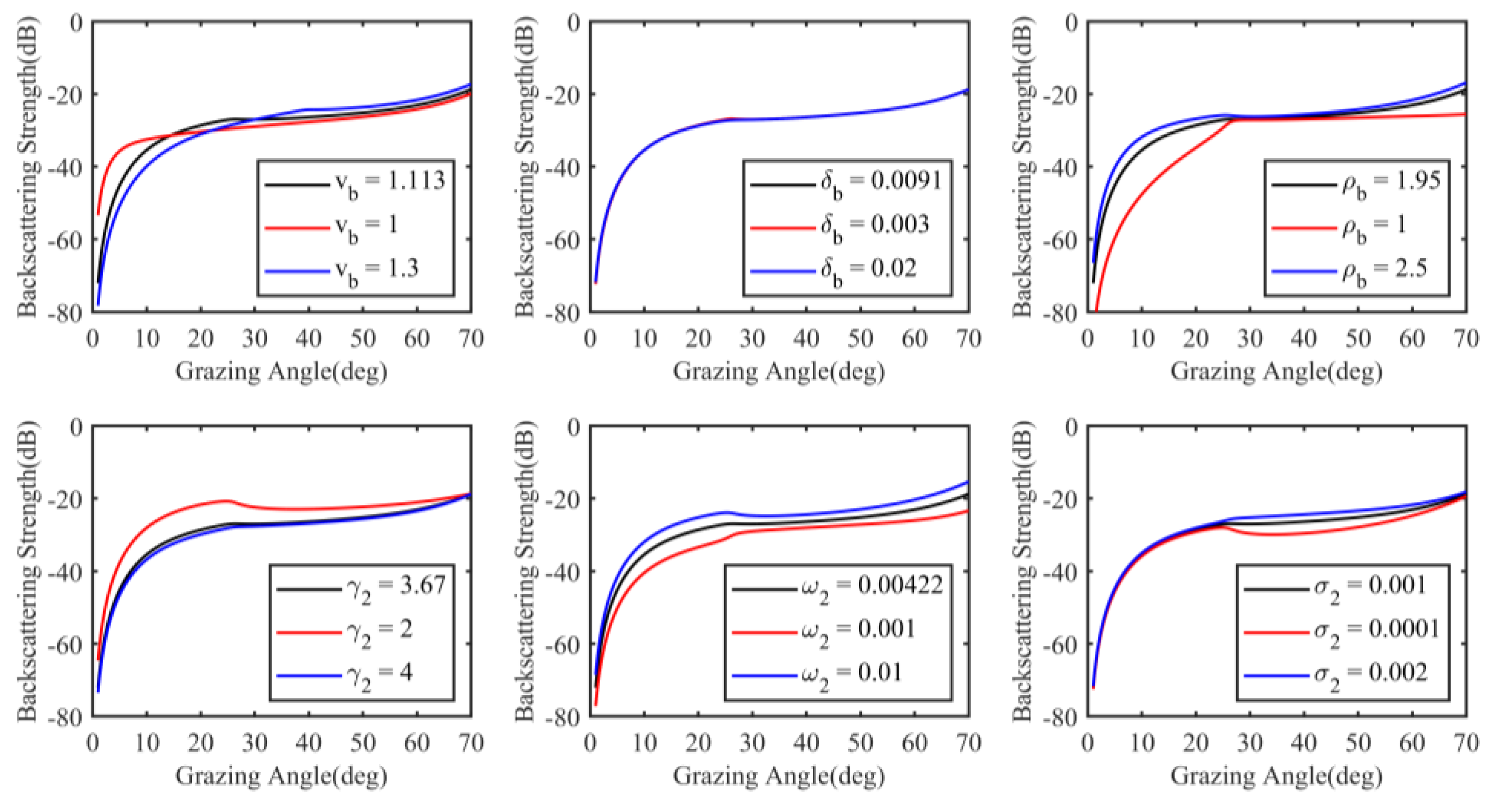
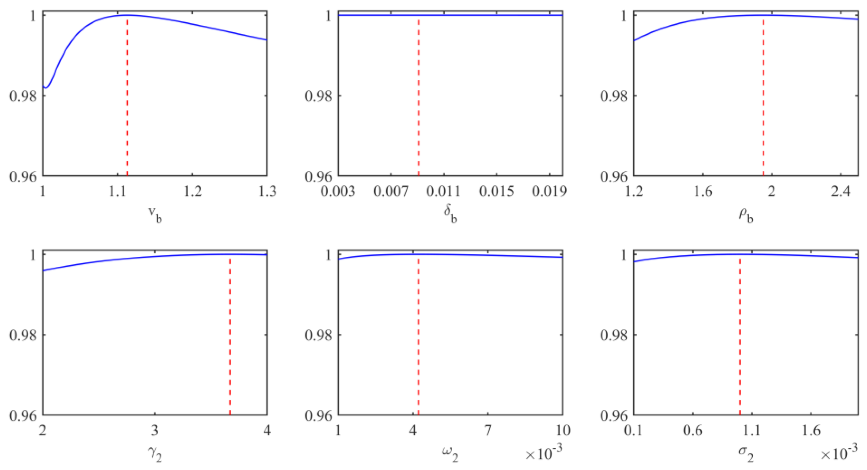
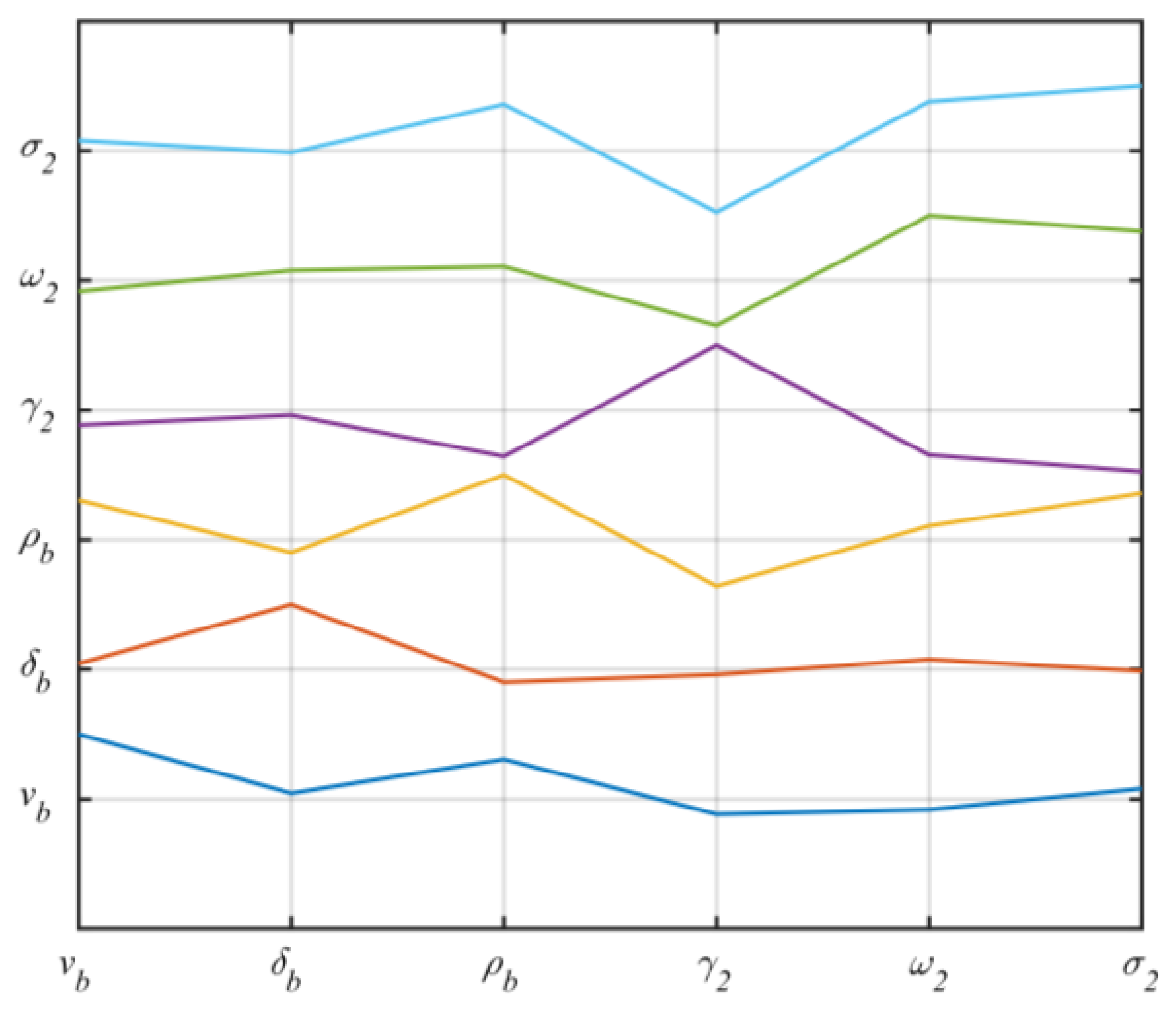
4.1. Sensitivity Analysis

Before conducting the numerical simulation study, it is important to consider the sensitivity of the inversion parameters. Through sensitivity analysis, we can further guide inversion and understand which parameters are most likely to be accurately inverted before inversion. At the same time, we can also provide some explanation for the inversion results [32,33]. In this study, the seabed is modeled as a half-space with a rough interface at the seafloor and volume inhomogeneities within the half-space. As described in Section 2, we employed the acoustic backscattering model as a forward model. We selected the inversion parameters as the sediment/water sound speed ratio $v_b$, loss parameter ${\delta }_b$ associated with sediment attenuation, sediment/water density ratio ${\rho }_b$, spectral strength $w_2$ and the spectral exponent ${\gamma }_2$ used to characterize seafloor roughness, and volume scattering cross section/attenuation coefficient ratio ${\sigma }_2$ associated with the sediment volume scattering characteristics.

We analyzed the sensitivity of the inversion parameters to the backscattering model and the objective function from both qualitative and quantitative perspectives. The simulation parameters were selected from [34], and the corresponding true values and search ranges are listed in

Table 1. Inversion results of the numerical simulation.

Bottom Parameter	Symbol	Unit	True Value	Search Range	Mean ± Standard Deviation	MAP
Sediment/water sound speed ratio	$v_b$	dimensionless	1.113	1–1.3	1.115 ± 0.004	1.116
Loss parameter of sediment	${\delta }_b$	dimensionless	0.0091	0.003–0.02	0.0060 ± 0.0030	unclear
Sediment/water density ratio	${\rho }_b$	dimensionless	1.95	1–2.5	1.95 ± 0.12	1.96
Spectral exponent of roughness spectrum	${\gamma }_2$	dimensionless	3.67	2–4	3.54 ± 0.23	-
Spectral strength of roughness spectrum	$w_2$	cm4	0.00422	0.001–0.01	0.00391 ± 0.00092	0.00425
Volume scattering cross-section/attenuation coefficient ratio	${\sigma }_2$	dimensionless	0.001	0.0001–0.002	0.0011 ± 0.0005	unclear

. The sediment type chosen was fine sand. The search ranges for the inversion parameters have been reasonably selected based on the typical range of fine sandy sediments. The frequency was set as $f=35 \mathrm{k}\mathrm{H}\mathrm{z}$, the grazing angle range was 0°–70°, and the sound speed in seawater was set as 1487 m/s. First, we qualitatively analyzed the sensitivity of the inversion parameters to the backscattering model. By utilizing the control variable method, keeping other parameters fixed at their true values, we computed the backscattering strength for the upper and lower bounds of each parameter separately using Equation (1). The backscattering strength variation with each parameter is shown in Figure 2. In these figures, the red solid line represents the variation of the backscattering strength with the grazing angle at the lower boundary of each parameter, the blue solid line denotes the variation at the upper boundary, and the black solid line indicates the variation of backscattering strength when each parameter is set to be the simulated true value. Comparison of these results shows that the backscattering strength is strongly dependent on three parameters: $v_b$, ${\rho }_b$, and $w_2$. Although ${\gamma }_2$ also exhibits obvious variation in the backscattering strength values, its true value is close to the upper boundary (the finite boundary value being determined by its physical properties). The sensitivity of ${\gamma }_2$ needs to be further analyzed. When the grazing angle is in the range of 25°–60°, the change in backscattering strength caused by ${\sigma }_2$ is notable. In contrast, the effects caused by ${\delta }_b$ are so weak that they are barely noticeable.

Figure 3 shows the variation in the Bartlett correlation with each parameter based on the objective function to quantitatively analyze the sensitivity of each parameter. The red vertical dotted line represents the true value, and the blue solid line denotes the parameter sensitivity curve at 35 kHz. These results indicate that parameters $v_b$, ${\rho }_b$, and ${\gamma }_2$ are all sensitive within the parameter search ranges, which is consistent with the above results. A further novel finding is that the sensitivity of ${\gamma }_2$ is very weak in the search range from 3 to 4. Therefore, we sorted it to be a weakly sensitive parameter. In contrast to the qualitative analysis results mentioned above, $w_2$ does not exhibit strong sensitivity, and ${\sigma }_2$ has a very weak sensitivity. ${\delta }_b$ is still insensitive.

In general, we classified the inversion parameters into three categories according to their sensitivities: $v_b$ and ${\rho }_b$ are considered sensitive parameters; ${\gamma }_2$, $w_2$, and ${\sigma }_2$ are weakly sensitive parameters, and ${\delta }_b$ is insensitive. For these sensitive parameters, it is expected that more accurate results will be obtained through inversion.

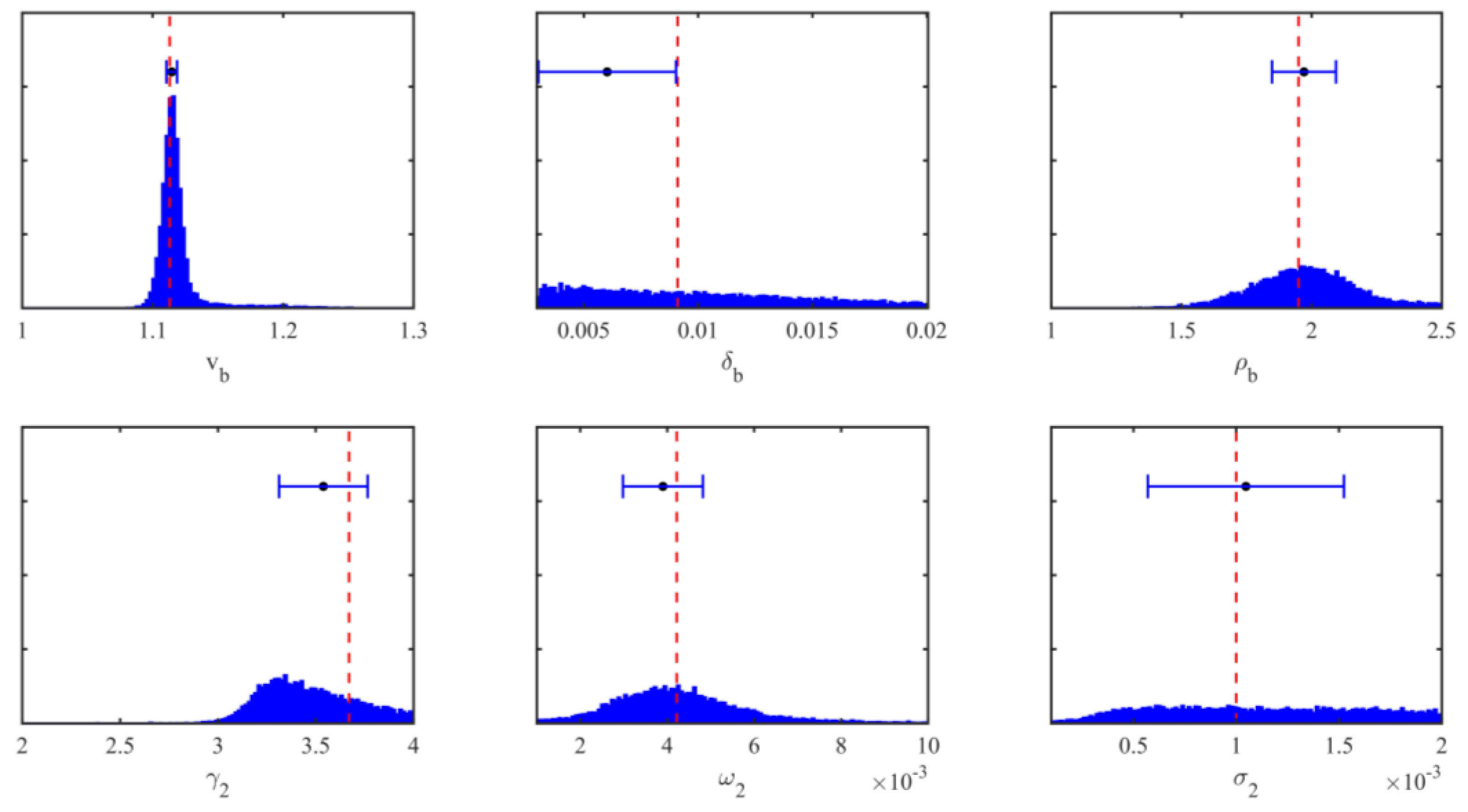
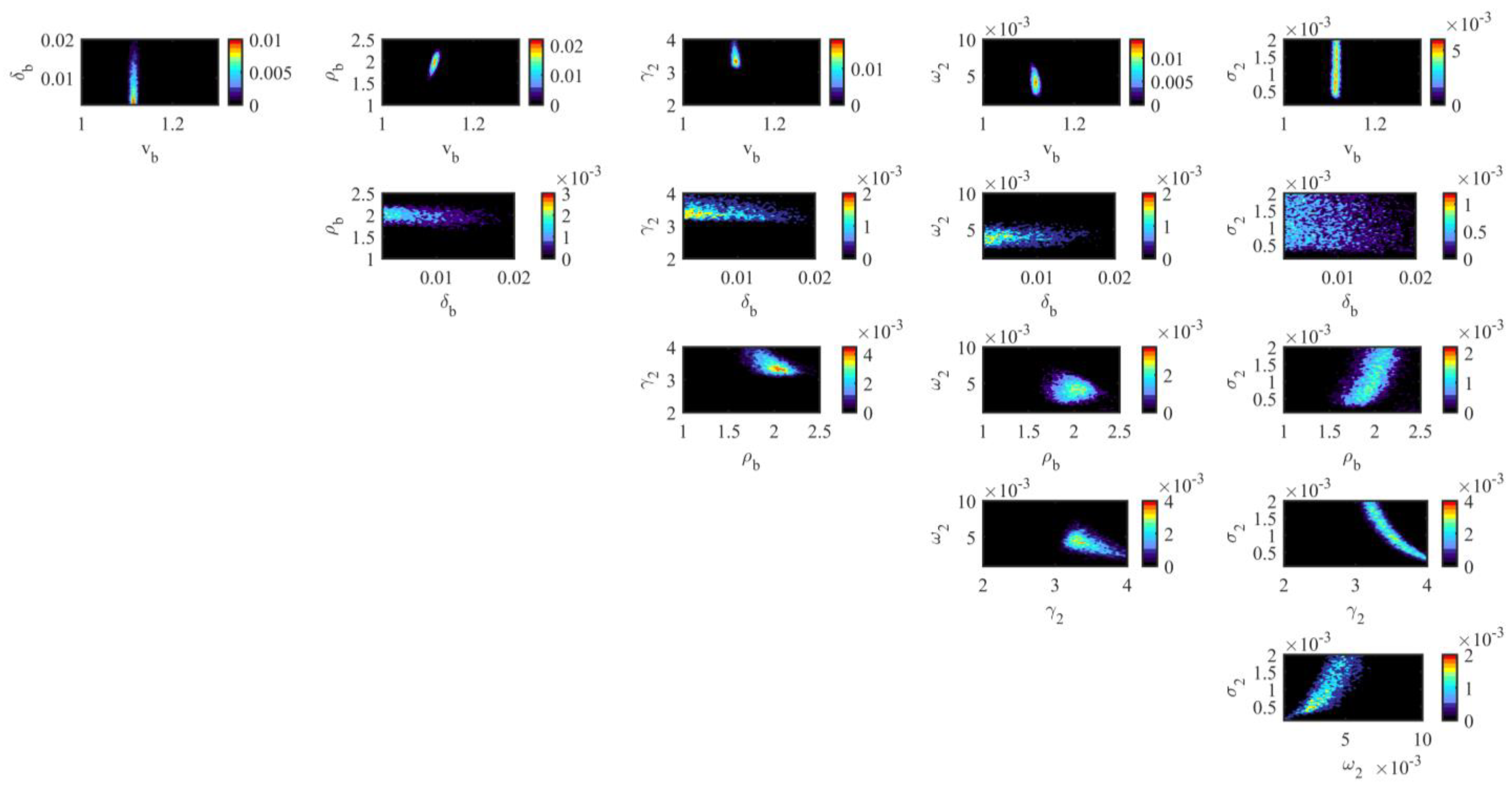
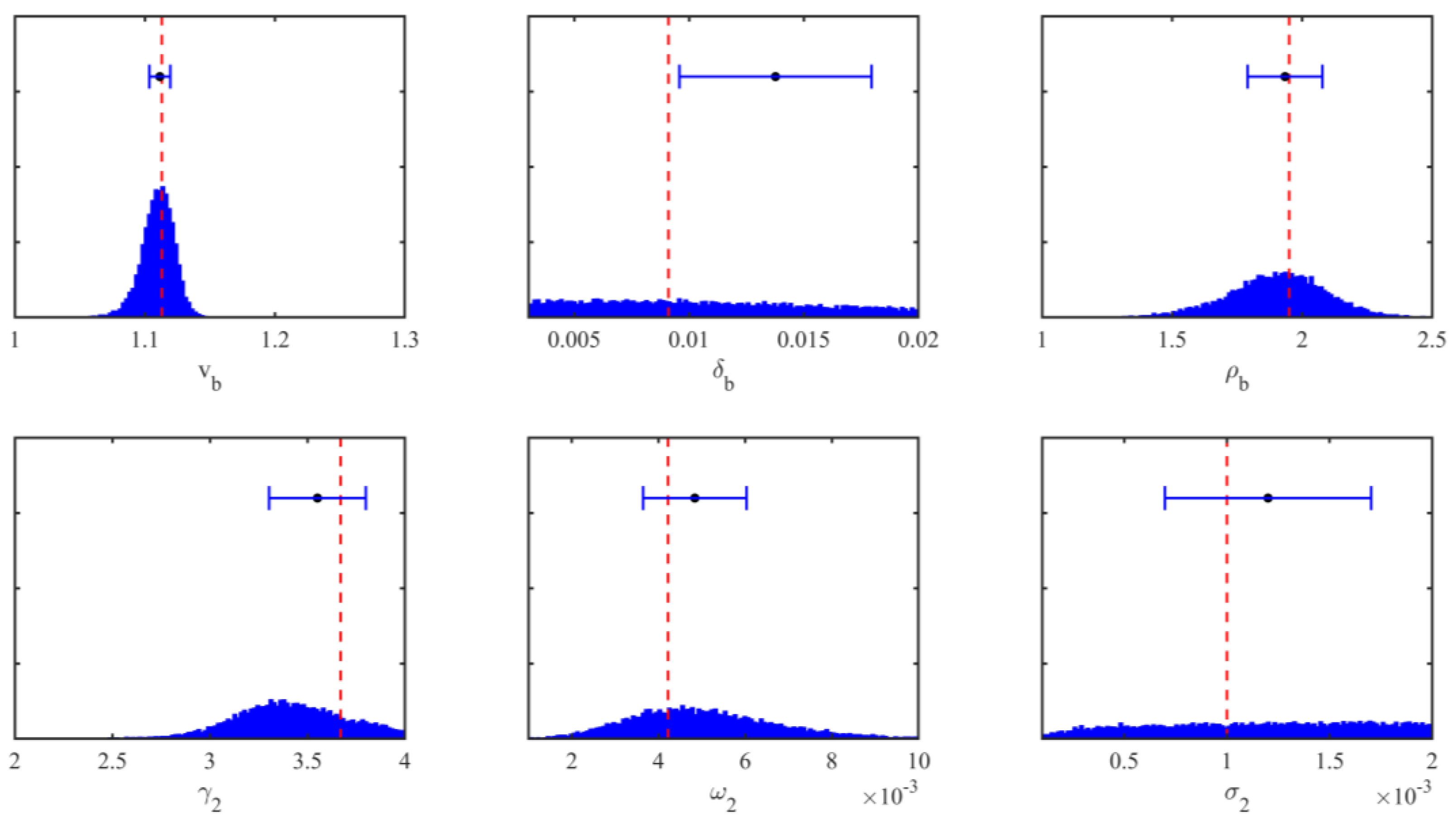
4.2. Analysis of Simulation Results

In this section, the feasibility of the multiparameter Bayesian inversion method proposed in this study will be validated through numerical simulation. In the numerical simulation, we employed a Gaussian random variable with a mean value of zero and a standard deviation of $\sigma$ to simulate the data error. Subsequently, the measured data can be expressed as follows:

$$d_f=p_f\left(\mathbf{m}\right)+\xi \sigma ,$$

(28)

where $\xi$ is a one-dimensional (1D) random variable that is subjected to a standard normal distribution and $\sigma$ is set to be 1.2 dB.

The 1D marginal PPDs obtained by using the Bayesian inversion based on the FGS method are shown in Figure 4. For these figures, the simulated true values of the parameters are plotted as red vertical dashed lines, the black solid circles represent the mean values obtained by using the FGS, and the blue error bars stand for the standard deviation. The standard deviation corresponds to the 70% confidence interval. It is found that the true values are basically consistent with the peaks of the 1D marginal PPD and the mean values for the sensitive parameters $v_b$ and ${\rho }_b$, and compared to ${\rho }_b$, $v_b$ has less uncertainty. Here we extract the MAP as the best estimate for $v_b$ and ${\rho }_b$. For the weakly sensitive parameters ${\gamma }_2$, $w_2$, and ${\sigma }_2$, their true values are all within the confidence interval. However, the 1D marginal PPD of ${\sigma }_2$ is smoother and has greater uncertainty, and its 1D marginal PPD tends to be uniform, making the MAP unclear. Therefore, we choose the mean value as the inversion result for ${\sigma }_2$. There is some deviation between the true value and the peaks of the 1D marginal PPD for the parameter ${\gamma }_2$, and its distribution is not nearly symmetrical, possibly because the parameter ${\gamma }_2$ is relatively insensitive in the search range of 3 to 4. Therefore, we choose the mean value as the best estimate for ${\gamma }_2$. In addition, the true value is basically consistent with the peaks of the 1D marginal PPD for the parameter $w_2$, and we extract the MAP as its best estimate. The 1D marginal PPD of the insensitive parameter ${\delta }_b$ is relatively flat and has a wide distribution; this shows significant uncertainty. Moreover, the true value of ${\delta }_b$ is not within the confidence interval, indicating that the inversion result is unreliable. Here we take the mean value as its inversion numerical result. In general, the inversion results are as expected based on the above sensitivity analysis. Table 1 lists the MAP, the mean values and standard deviations of the inversion results obtained by using the Bayesian inversion based on the FGS method.

To quantitatively analyze the correlations between the various parameters, the normalized covariance matrix is shown in Figure 5, where the diagonal part represents the autocorrelation coefficient of the parameters. Figure 6 shows the 2D marginal PPDs of the specified parameter pairs obtained by using Bayesian inversion based on the FGS method, that is, the joint marginal PPD of the pairwise parameters. It is obvious that reasonably strong positive correlations exist between $v_b$ and ${\rho }_b$ and between ${\sigma }_2$ and the two parameters ${\rho }_b$ and $w_2$, whereas strong negative correlations exist between ${\gamma }_2$ and the three parameters ${\rho }_b$, ${\sigma }_2$, and $w_2$. The insensitive parameter ${\delta }_b$ is uncorrelated with other parameters. It is worth noting that the correlation between the parameters is related to the physical environment of the bottom, and this correlation can be interpreted based on the variation in the backscattering strength with each parameter [18]. To overcome the influence of the correlation on the inversion results, it is imperative to acquire more prior information during the inversion process.

5. Validation with Historical Backscattering Data

5.1. Experiment Data Description

The experimental data were derived from the Quinault Range site, which is one of the five high-frequency acoustic experiment sites with different sediment types conducted by the U.S. Navy Research Laboratory (NRL). The objective of these experiments was to quantitatively assess environmental parameters in order to comprehend the fundamental mechanism of and to model bottom high-frequency scattering. The Quinault Range site is located 17 km west of the Washington coast at an average water depth of 49 m (for experimental location details, please refer to Figure 1 in reference [34]). The main sedimentary component of this site is fine sand. An analysis of numerous samples collected in the experiment indicates that the geoacoustic characteristics of this area are homogeneous and that there is no significant gradient variation in physical parameters within the sediment. This provides a good environmental condition for the acoustic backscattering model mentioned in Section 2.

To obtain geoacoustic and physical parameters of the sediment, a boxcore sampling technique was employed at the Quinault Range site. The compressional wave speed and attenuation of the sediment were measured using a pulse technique through the sediment cores, while other physical parameters, such as the sediment density, were measured by slicing core samples. In addition, seafloor roughness was measured photogrammetrically to estimate the roughness power spectra characteristic of the sediments. Backscattering strength was measured at the Quinault Range site using a towed platform described in reference [29]. Specific experimental details and data processing methods are described in reference [34] and will not repeated here.

Table 2. Inversion results of the experimentally measured data.

Bottom Parameter	Symbol	Unit	True Value	Search Range	Mean ± Standard Deviation	MAP
Sediment/water sound speed ratio	$v_b$	dimensionless	1.113	1–1.3	1.112 ± 0.008	1.114
Loss parameter of sediment	${\delta }_b$	dimensionless	0.0091	0.003–0.02	0.0138 ± 0.0042	unclear
Sediment/water density ratio	${\rho }_b$	dimensionless	1.95	1–2.5	1.94 ± 0.14	1.93
Spectral exponent of roughness spectrum	${\gamma }_2$	dimensionless	3.67	2–4	3.42 ± 0.25	-
Spectral strength of roughness spectrum	$w_2$	cm4	0.00422	0.001–0.01	0.00481 ± 0.00123	0.00462
Volume scattering cross-section/attenuation coefficient ratio	${\sigma }_2$	dimensionless	0.001	0.0001–0.002	0.0012 ± 0.0005	unclear

presents the input parameters utilized for the data-model comparisons as detailed in reference [34] measured at the Quinault Range site, which are used as actual values for a comparison of inversion results in this paper. It should be further noted that, apart from the spectral strength, all parameters are dimensionless and considered independent of the acoustic frequency. And the spectral strength and spectral exponent of the roughness spectrum were derived from longitudinal measurements (as the anisotropy between the transverse and longitudinal directions are negligible).

Backscattering strengths at 35 kHz were extracted from reference [34] to validate the proposed inversion method. Based on the seabed half-space assumption proposed in Section 4.1, we integrate the acoustic backscattering model discussed in Section 2 with the input parameters listed in Table 2 to calculate backscattering strengths at 35 kHz. The comparison of the measured data and model-predicted results is shown in Figure 7. In contrast to the approach in which the composite roughness model was used to address roughness scattering in reference [34], we employed the small-roughness perturbation approximation mentioned in Section 2.1. Equations (1) and (10) were used to calculate the total backscattering strengths and volume scattering strengths, respectively, which was consistent with the treatment methods in reference [34]. The blue inverted triangles indicate the measured backscattering strengths, the red solid lines represent the total backscattering strengths predicted by the model, and the black and blue dashed lines indicate the backscattering strengths derived from the roughness and volume scattering, respectively. It can be found that the roughness scattering is the primary scattering mechanism, whereas volume scattering makes a smaller contribution to the overall backscattering strength.

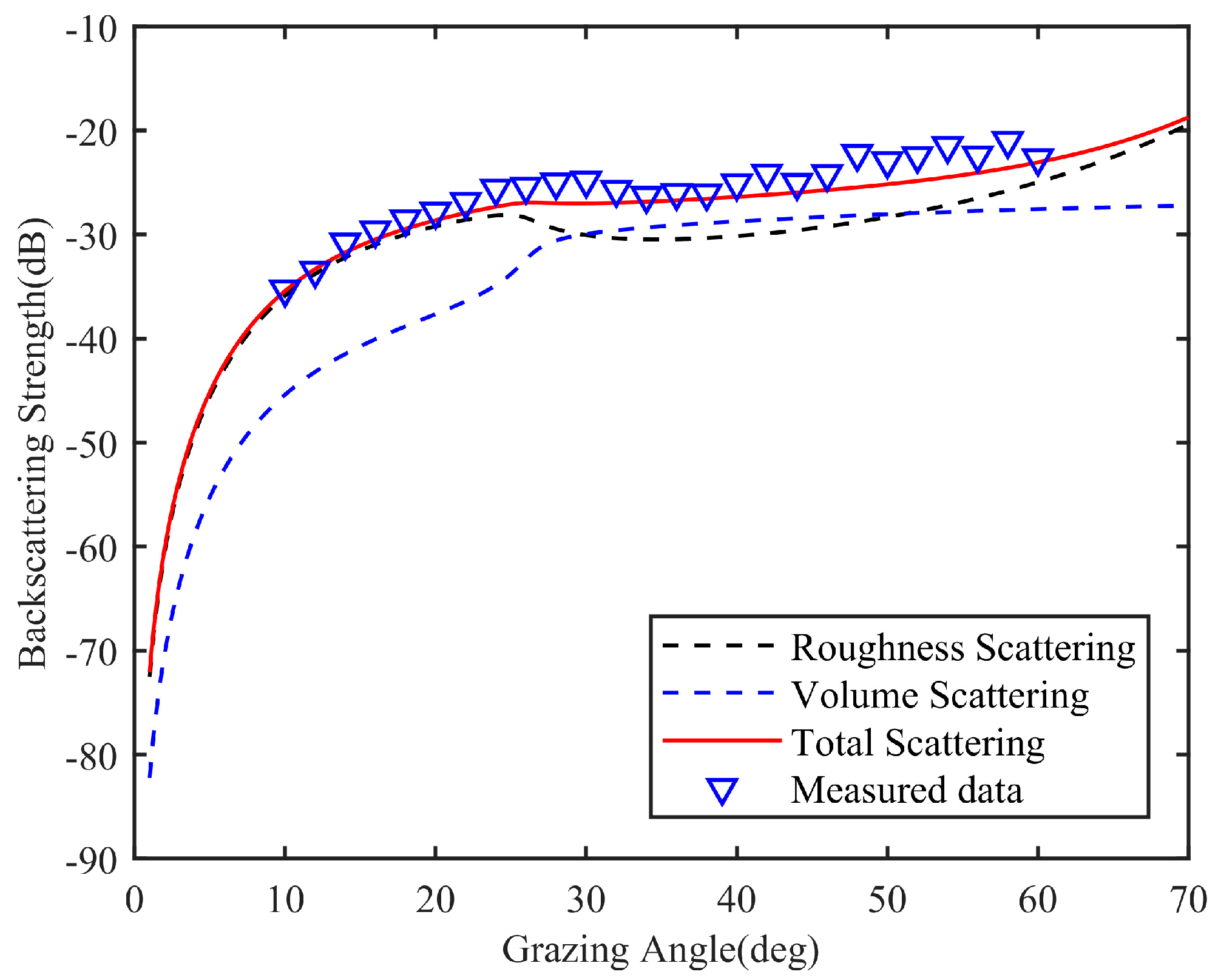
5.2. Analysis of Experiment Results

We conducted acoustic inversion of the six parameters of the Quinault Range site using the proposed method in a manner similar to that in the simulation study. The 1D marginal PPDs derived from the Bayesian inversion based on the FGS method are shown in Figure 8. Compared with the numerical simulation results in Section 4.2, the 1D marginal PPD distribution of the parameters in Figure 8 is slightly wider, indicating an increase in uncertainty. The reason for the discrepancy is that the data errors are larger than those in the numerical simulation. The true values are basically consistent with the peaks of the 1D marginal PPDs and the mean values for the sensitive parameters $v_b$ and ${\rho }_b$, indicating reliable inversion results, and $v_b$ has less uncertainty than ${\rho }_b$. This conclusion agrees well with the numerical simulation results. For the weakly sensitive parameters ${\gamma }_2$ and $w_2$, the peaks of the 1D marginal PPDs depart from the true values, but the true values are within the confidence interval. This result is basically consistent with the results obtained from the backscattering model inversion in Steninger et al.’s paper [35], but due to different intermediate processes, such as the objective function employed and the geoacoustic model used, there may be some differences in the PPD distribution. In contrast, the weakly sensitive parameter ${\sigma }_2$ and the insensitive parameter ${\delta }_b$ exhibit widely distributed 1D marginal PPDs and relatively large uncertainties, and the inversion result of the insensitive parameter ${\delta }_b$ meets our expectations. Based on the numerical simulation research results in Section 4.2, we attempt to provide such a guideline: 1. for the 1D marginal PPDs with obvious characteristics and approximate symmetry, the MAP is used as the best estimate value; 2. for the 1D marginal PPDs with obvious characteristics, but its distribution is not nearly symmetrical, the mean value is selected as the optimal estimation value; and 3. for the 1D marginal PPDs that are relatively uniform, the mean value is used as its inversion result. Therefore, we take the MAP as the best estimate for $v_b$, ${\rho }_b$, and $w_2$, using the mean value as the inversion results for ${\gamma }_2$, ${\sigma }_2$, and ${\delta }_b$. Table 2 presents the MAP, along with the mean values and standard deviations, of the inversion results derived by employing the Bayesian inversion method.

The normalized covariance matrix is shown in Figure 9. The 2D marginal PPDs of the specified parameter pair obtained using the Bayesian inversion based on the FGS method are given Figure 10. The figures reveal that ${\rho }_b$ is positively correlated with $v_b$ and with ${\sigma }_2$, ${\gamma }_2$ is positively correlated with $w_2$, and ${\gamma }_2$ is negatively correlated with ${\sigma }_2$. A comparison with the numerical simulation shows that the correlations between some parameters decrease.

Figure 11 shows the comparison of the predicted backscattering strengths with the mean of the inversion results as the model input and the measured backscattering strength at the Quinault Range site. The results agree with each other.

6. Conclusions

To accurately obtain bottom multi-parameter and analyze the uncertainties and correlations of inversion results, we proposed a Bayesian inversion method based on an acoustic backscattering model. The inversion employed the FGS sampling method to estimate the MAP, the mean values and standard deviations of the inversion results. Experimental data from the Quinault Range site are used to validate the inversion method. Simulation and experiment results show that the method can effectively be applied to bottom multi-parameter inversion, except for the insensitive parameter ${\delta }_b$. Furthermore, the predicted bottom backscattering strengths using the inversion results are basically consistent with the actual measured values.

The sensitivity analysis results indicate that $v_b$ and ${\rho }_b$ are sensitive parameters; ${\gamma }_2$, $w_2$, and ${\sigma }_2$ are weakly sensitive parameters, and ${\delta }_b$ is insensitive. In the inversion results, we employ the MAP as the best estimate for the sensitive parameters $v_b$ and ${\rho }_b$ and the weakly sensitive parameters $w_2$, using the mean value as the inversion results for the weakly sensitive parameters ${\gamma }_2$ and ${\sigma }_2$ and the insensitive parameter ${\delta }_b$. Upon analyzing the uncertainties and correlations within the inversion results, it becomes evident that the experimental data’s larger errors significantly contribute to the heightened uncertainty of the inversion results. Meanwhile, the correlation between some parameters decreases. This contrasts the numerical simulations with relatively minimal errors. In the future, we will further use multifrequency data to enhance the accuracy and reliability of the inversion results.

References

1. Jackson, D.; Richardson, M. High-Frequency Seafloor Acoustics; Springer Science & Business Media: Berlin/Heidelberg, Germany, 2007. [Google Scholar]
2. Colin, M.; Otnes, R.; van Walree, P.; Prior, M.; Dol, H.; Ainslie, M. From sonar performance modelling to underwater communication performance modelling. In Proceedings of the 4th Underwater Acoustics Conference and Exhibition, Skiathos, Greece, 3–8 September 2017; pp. 221–228. [Google Scholar]
3. Lynch, J.; Tang, D. Overview of Shallow Water 2006 JASA EL Special Issue Papers. J. Acoust. Soc. Am. 2008, 124, EL63–EL65. [Google Scholar] [CrossRef] [PubMed]
4. Lee, K.M.; Ballard, M.S.; McNeese, A.R.; Muir, T.G.; Wilson, P.S.; Costley, R.D.; Hathaway, K.K. In situ measurements of sediment acoustic properties in Currituck Sound and comparison to models. J. Acoust. Soc. Am. 2016, 140, 3593–3606. [Google Scholar] [CrossRef] [PubMed]
5. Jiang, Y.-M.; Holland, C.W.; Dosso, S.E.; Dettmer, J. Depth and frequency dependence of geoacoustic properties on the New England Mud Patch from reflection coefficient inversion. J. Acoust. Soc. Am. 2023, 154, 2383–2397. [Google Scholar] [CrossRef] [PubMed]
6. Dosso, S.E.; Yeremy, M.L.; Ozard, J.M.; Chapman, N.R. Estimation of ocean-bottom properties by matched-field inversion of acoustic field data. IEEE J. Oceanic. Eng. 1993, 18, 232–239. [Google Scholar] [CrossRef]
7. Liu, M.; Niu, H.; Li, Z.; Liu, Y.; Zhang, Q. Deep-learning geoacoustic inversion using multi-range vertical array data in shallow water. J. Acoust. Soc. Am. 2022, 151, 2101–2116. [Google Scholar] [CrossRef] [PubMed]
8. Chapman, N.R.; Shang, E.C. Review of Geoacoustic Inversion in Underwater Acoustics. J. Theor. Comput. Acoust. 2021, 29, 66. [Google Scholar] [CrossRef]
9. Uscinski, B.J. Matched Field Processing for Underwater Acoustics. By ALEXANDRA TOLSTOY. World Scientific, 1993. 212 pp. J. Fluid Mech. 1994, 259, 375. [Google Scholar] [CrossRef]
10. Shi, J.; Sun, D.; Dosso, S.E.; Liu, Q. Geoacoustic inversion of the pressure gradient data using a single vector sensor. J. Acoust. Soc. Am. 2018, 144, 1974. [Google Scholar] [CrossRef]
11. Jiang, Y.-M.; Holland, C.W.; Dosso, S.; Dettmer, J. Bayesian geoacoustic inversion of 1–2 kHz seabed reflection data for layered muddy sediments. J. Acoust. Soc. Am. 2022, 152, A145. [Google Scholar] [CrossRef]
12. Xue, Y.; Zhu, H.; Wang, X.; Zheng, G.; Liu, X.; Wang, J. Bayesian geoacoustic parameters inversion for multi-layer seabed in shallow sea using underwater acoustic field. Front. Mar. Sci. 2023, 10, 1058542. [Google Scholar] [CrossRef]
13. Jackson, D.R.; Baird, A.M.; Crisp, J.J.; Thomson, P.A.G. High-frequency bottom backscatter measurements in shallow water. J. Acoust. Soc. Am. 1986, 80, 1188–1199. [Google Scholar] [CrossRef]
14. Williams, K.L.; Jackson, D.R.; Thorsos, E.I.; Dajun, T.; Briggs, K.B. Acoustic backscattering experiments in a well characterized sand sediment: Data/model comparisons using sediment fluid and Biot models. IEEE J. Oceanic. Eng. 2002, 27, 376–387. [Google Scholar] [CrossRef]
15. Radhakrishnan, S.; Anu, A.P. Characterization of seafloor roughness from high-frequency acoustic backscattering measurements in shallow water off the west coast of India. J. Acoust. Soc. Am. 2020, 148, 2987–2996. [Google Scholar] [CrossRef] [PubMed]
16. Turgut, A. Inversion of bottom/subbottom statistical parameters from acoustic backscatter data. J. Acoust. Soc. Am. 1997, 102, 833–852. [Google Scholar] [CrossRef]
17. Zou, B.; Zhai, J.; Qi, Z.; Li, Z. A Comparison of Three Sediment Acoustic Models Using Bayesian Inversion and Model Selection Techniques. Remote Sens. 2019, 11, 562. [Google Scholar] [CrossRef]
18. Yu, S.; Liu, B.; Yu, K.; Yang, Z.; Kan, G.; Zong, L. Inversion of bottom parameters using a backscattering model based on the effective density fluid approximation. Appl Acoust 2021, 182, 108187. [Google Scholar] [CrossRef]
19. Dosso, S.E.; Nielsen, P.L.; Harrison, C.H. Bayesian inversion of reverberation and propagation data for geoacoustic and scattering parameters. J. Acoust. Soc. Am. 2009, 125, 2867–2880. [Google Scholar] [CrossRef]
20. Gerstoft, P.; Mecklenbräuker, C.F. Ocean acoustic inversion with estimation of a posteriori probability distributions. J. Acoust. Soc. Am. 1998, 104, 808–819. [Google Scholar] [CrossRef]
21. Lapinski, A.L.S.; Dosso, S.E. Bayesian geoacoustic inversion for the Inversion Techniques 2001 Workshop. IEEE J. Oceanic. Eng. 2003, 28, 380–393. [Google Scholar] [CrossRef]
22. Dosso, S.E. Quantifying uncertainty in geoacoustic inversion. I. A fast Gibbs sampler approach. J. Acoust. Soc. Am. 2002, 111, 129–142. [Google Scholar] [CrossRef]
23. Dosso, S.E.; Nielsen, P.L. Quantifying uncertainty in geoacoustic inversion. II. Application to broadband, shallow-water data. J. Acoust. Soc. Am. 2002, 111, 143–159. [Google Scholar] [CrossRef] [PubMed]
24. Malinverno, A. A Bayesian criterion for simplicity in inverse problem parametrization. Geophys. J. Int. 2000, 140, 267–285. [Google Scholar] [CrossRef]
25. Ivakin, A.N. A unified approach to volume and roughness scattering. J. Acoust. Soc. Am. 1998, 103, 827–837. [Google Scholar] [CrossRef]
26. Jackson, D.R.; Briggs, K.B.; Williams, K.L.; Richardson, M.D. Tests of models for high-frequency seafloor backscatter. IEEE J. Oceanic. Eng. 1996, 21, 458–470. [Google Scholar] [CrossRef]
27. Williams, K.L.; Jackson, D.R. Bistatic bottom scattering: Model, experiments, and model/data comparison. J. Acoust. Soc. Am. 1998, 103, 169–181. [Google Scholar] [CrossRef]
28. Yu, S.; Liu, B.; Yu, K.; Yang, Z.; Kan, G.; Zhang, X. Comparison of acoustic backscattering from a sand and a mud bottom in the South Yellow Sea of China. Ocean Eng. 2020, 202, 107145. [Google Scholar] [CrossRef]
29. Jackson, D.R.; Winebrenner, D.P.; Ishimaru, A. Application of the composite roughness model to high-frequency bottom backscattering. J. Acoust. Soc. Am. 1986, 79, 1410–1422. [Google Scholar] [CrossRef]
30. Olson, D.R. A series approximation to the Kirchhoff integral for Gaussian and exponential roughness covariance functions. J. Acoust. Soc. Am. 2021, 149, 4239–4247. [Google Scholar] [CrossRef]
31. Battle, D.J.; Gerstoft, P.; Hodgkiss, W.S.; Kuperman, W.A.; Nielsen, P.L. Bayesian model selection applied to self-noise geoacoustic inversion. J. Acoust. Soc. Am. 2004, 116, 2043–2056. [Google Scholar] [CrossRef]
32. Sanjana, M.; Latha, G.; Potty, G.R. Sensitivity analysis of model parameters in geoacoustic inversion. In 2013 Ocean Electronics (SYMPOL); IEEE: Piscataway, NJ, USA, 2013; pp. 96–100. [Google Scholar]
33. Wan, L.; Badiey, M.; Knobles, D.P.; Wilson, P.S. The Airy phase of explosive sounds in shallow water. J. Acoust. Soc. Am. 2018, 143, EL199–EL205. [Google Scholar] [CrossRef]
34. Briggs, K.B. High-Frequency Acoustic Scattering from Sediment Interface Roughness and Volume Inhomogeneities; Stennis Space Center, MS: Naval Research Laboratory: Coral Gables, FL, USA, 1994. [Google Scholar]
35. Steininger, G.; Dettmer, J.; Dosso, S.E.; Holland, C.W. Trans-dimensional joint inversion of seabed scattering and reflection data. J. Acoust. Soc. Am. 2013, 133, 1347–1357. [Google Scholar] [CrossRef] [PubMed]
Figure 1. Definition of angles used in treating scattering.
Jmse 12 00629 g001
Figure 2. Backscattering strength variation with each parameter.
Jmse 12 00629 g002
Figure 3. Variation in the Bartlett correlation for each parameter (the blue solid line denotes the parameter sensitivity curve, and the true values are indicated by the vertical red dashed line).
Jmse 12 00629 g003
Figure 4. The mean values and standard deviations of the inversion results (black dot with blue error bars), and the 1D marginal PPDs for each parameter (true values are indicated by the vertical red dashed line).
Jmse 12 00629 g004
Figure 5. Diagram of the normalized covariance matrix of inversion parameters.
Jmse 12 00629 g005
Figure 6. Two-dimensional marginal PPDs of specified pairs of parameters.
Jmse 12 00629 g006
Figure 7. Comparison of the measured and the model-predicted backscattering strengths at 35 kHz.
Jmse 12 00629 g007
Figure 8. The mean values and standard deviations of the inversion results (black dot with blue error bars), and the 1D marginal PPDs for each parameter derived from measured backscattering strength (true values are indicated by the vertical red dashed line).
Jmse 12 00629 g008
Figure 9. Diagram of the normalized covariance matrix of inversion parameters derived from the measured backscattering strength.
Jmse 12 00629 g009
Figure 10. Two-dimensional marginal PPDs of specified pairs of parameters derived from the measured backscattering strengths.
Jmse 12 00629 g010
Figure 11. Comparison of the predicted and measured backscattering strengths.
Jmse 12 00629 g011