Asymptotic Ray Method for the Double Square Root Equation

Abstract

The parabolic wave equation describes wave propagation in a preferable direction, which is usually horizontal in underwater acoustics and vertical in seismic applications. For dense receiver arrays (receiver spacing is less than signal wavelength), this equation can be used for propagating the recorded wavefield back into the medium for imaging sources and scattering objects. Similarly, for multiple source and receiver array acquisition, typical for seismic exploration and potentially beneficial for ocean acoustics, one can model data in one run using an extension of the parabolic equation—the pseudo-differential Double Square Root (DSR) equation. This extended equation allows for the modeling and imaging of multi-source data but operates in higher-dimensional space (source, receiver coordinates, and time), which makes its numerical computation time-consuming. In this paper, we apply a faster ray method for solving the DSR equation. We develop algorithms for both kinematic and dynamic ray tracing applicable to either data modeling or true-amplitude recovery. Our results can be used per se or as a basis for the future development of more elaborated asymptotic techniques that provide accurate and computationally feasible results.

1. Introduction

The parabolic wave equation, also known as the one-way or Single Square Root equation, describes wave propagation in a preferable direction, which is usually horizontal in underwater acoustics [1] and vertical in seismic applications [2]. There is another use for this equation that relates to data recorded by dense receiver arrays (receiver spacing is less than the signal wavelength): hydrophone arrays in water column or ocean bottom cables in seismic studies. Then, the parabolic wave equation can be used for propagating the recorded wavefield back from the array towards the source (backwards in time and the preferable direction). Such back-propagation can be used for the localization of active sources and scattering of objects in acoustics [3] or for the imaging of geological boundaries in seismic applications [4]. Studying 3D heterogeneous models requires more data from multiple source and receiver arrays. Such acquisition geometry is widely used in seismic exploration [5] and may be beneficial for ocean acoustics [6], where it would necessitate a vertical receiver array with an active source firing at several depths along the same array. The data recorded in this way depend on both the source and the receiver coordinates, and one can back-propagate these data using the extended parabolic equation—the pseudo-differential Double Square Root (DSR) equation [2].

The kinematics of the DSR equation was first described in [7], and its pseudo-differential version was later introduced by John Claerbout [2]. He used the DSR equation for the downward continuation of reflection–seismic data implementing the seismic imaging of subsurface geological structures (“survey-sinking” migration). This approach to seismic imaging is advantageous with respect to standard migration due to the simultaneous processing of all the data coming from different physical experiments, thus providing artifact-free images of the reflectors [8]. Alternatively, the DSR equation can be used for upward continuation and modeling seismic data following the “exploding reflector” concept [9]. Later on, a true-amplitude version of the DSR equation was derived from one-way wave equations [10,11,12], and its numerical implementation was discussed in [13,14]. The DSR migration was generalized to a VTI anisotropic case [15] and applied as a tool for migration velocity analysis [16]—a technique for the simultaneous recovery of the velocity model and the scatterer/reflector position. However, till now, DSR equation-based methods have found limited popularity due to prohibitively high computational costs, as they operate in higher-dimensional space (source, receiver coordinates, and time), especially in 3D settings [9].

For this paper, we applied the ray theory to find a high-frequency asymptotic solution to the DSR equation. We started from the true-amplitude DSR equation from [11] and the high-frequency asymptotics of the pseudo-differential operators from [10]. In our derivations, we followed Hamiltonian formalism, as presented in [17]. We developed formulae for high-frequency up/down data continuation that can be used for seismic modeling and imaging. We demonstrated the validity of our results with a series of numerical experiments. We restricted our considerations to a 2D case, postponing generalization to a 3D case for future work.

2. Materials and Methods

2.1. DSR Equation—Asymptotic Solution

In [11], the authors introduced a true-amplitude version of the DSR equation:

$$\left(\frac{\partial }{\partial z}-i{\mathsf{\Lambda }}_s-i{\mathsf{\Lambda }}_r-{\mathsf{\Gamma }}_s-{\mathsf{\Gamma }}_r\right)u=0,$$

(1)

where the Greek capital letters denote pseudo-differential operators, with the principal symbols being

$$\begin{gathered} i{\mathsf{\Lambda }}_{s/r}\leftrightarrow i{\lambda }_{s/r}\stackrel{\scriptscriptstyle\mathrm{def}}{=}\frac{i\omega }{v_{s/r}}\sqrt{1-\frac{v_{s/r}^2{k}_{s/r}^2}{{\omega }^2}}, \\ {\mathsf{\Gamma }}_{s/r}\leftrightarrow {\gamma }_{s/r}\stackrel{\scriptscriptstyle\mathrm{def}}{=}\frac{1}{2v_{s/r}}\frac{\partial v_{s/r}}{\partial z}·\left(1+\frac{v_{s/r}^2{k}_{s/r}^2}{{\omega }^2-v_{s/r}^2{k}_{s/r}^2}\right). \end{gathered}$$

(2)

Here and in the following, we shall use subscripts “$s$” and “$r$” for “source” and “receiver” coordinates, respectively, and slashes will indicate that either index can be chosen (self-consistently for the whole equation), meaning that

$$v_{s/r}\equiv v\left(x_{s/r},z\right)$$

(3)

is velocity at the point ${\left(x_{s/r},z\right)}^T$. Superscript $T$ stands for transposition. We denote angular frequency as $\omega$, the source and receiver wavenumbers as $k_{s/r}$, and the imaginary unit as $i$. Function $u\left(x_s,x_r,z,t\right)$ can be interpreted as the single-reflected acoustic pressure field initiated at point source ${\left(x_s,z\right)}^T$ and recorded at the receiver ${\left(x_r,z\right)}^T$.

Our derivation closely follows that from the first chapters in [17], which we shall further refer to as the “standard ray method”, and we recommend seeing [18] for more detailed consideration. We omit some proofs identical to those in the references above.

We seek the solution to (1) in the form of an asymptotic ray series:

$$\left\{\begin{array}{c}u\left(x_s,x_r,z,t\right)={\displaystyle \sum _{k=0}^{\infty }}{A}_k\left(x_s,x_r,z\right)F_k\left(t-\tau \left(x_s,x_r,z\right)\right),\\ \frac{d{F}_k}{dt}=F_{k-1}\hspace{1em}\forall k\ge 1,\end{array}\right.$$

(4)

where $A_k$ represents amplitude coefficients; $\tau$ represents two-way travel time, i.e., the time required for a wave to travel downward from the source to the reflecting interface and upward to the receiver array (different from the standard time variable in the wave equation); and functions $F_k$ denote the signal shape. The dynamics of the leading term of this ray series is characterized by the amplitude $A_0$.

Let us substitute solution (4) into the DSR Equation (1) and rearrange the coefficients corresponding to different $F_k$. This leads to an infinite system of equations for $\tau$ and $A_k$. The first equation controls the two-way travel time and will be referred to as the DSR eikonal equation:

$$\frac{\partial \tau }{\partial z}=-\sqrt{\frac{1}{v_s^2}-{\left(\frac{\partial \tau }{\partial x_s}\right)}^2}-\sqrt{\frac{1}{v_r^2}-{\left(\frac{\partial \tau }{\partial x_r}\right)}^2}.$$

(5)

The second equation controls the principal amplitude coefficient $A_0$ and will be referred to as the DSR transport equation:

$$〈{\nabla }_{\overrightarrow{x}}{A}_0,{\nabla }_{DSR}\tau 〉+\frac{1}{2}{A}_0〈{\nabla }_{\overrightarrow{x}},{\nabla }_{DSR}\tau 〉+\frac{1}{2}{A}_0{R}_{DSR}=0,$$

(6)

where we use the shortened notations ${\nabla }_{DSR}\tau$ and $R_{DSR}$:

$${\nabla }_{DSR}\tau \stackrel{\scriptscriptstyle\mathrm{def}}{=}\left[\begin{array}{c}\frac{\partial \tau }{\partial x_s}\left(1+\sqrt{\frac{\frac{1}{v_r^2}-{\left(\frac{\partial \tau }{\partial x_r}\right)}^2}{\frac{1}{v_s^2}-{\left(\frac{\partial \tau }{\partial x_s}\right)}^2}}\right)\\ \frac{\partial \tau }{\partial x_r}\left(1+\sqrt{\frac{\frac{1}{v_s^2}-{\left(\frac{\partial \tau }{\partial x_s}\right)}^2}{\frac{1}{v_r^2}-{\left(\frac{\partial \tau }{\partial x_r}\right)}^2}}\right)\\ \frac{\partial \tau }{\partial z}\end{array}\right],$$

(7)

$$R_{DSR}\stackrel{\scriptscriptstyle\mathrm{def}}{=}\frac{\frac{1}{v_s^3}\frac{\partial v_s}{\partial z}\sqrt{\frac{1}{v_r^2}-{\left(\frac{\partial \tau }{\partial x_r}\right)}^2}}{\frac{1}{v_s^2}-{\left(\frac{\partial \tau }{\partial x_s}\right)}^2}+\frac{\frac{1}{v_r^3}\frac{\partial v_r}{\partial z}\sqrt{\frac{1}{v_s^2}-{\left(\frac{\partial \tau }{\partial x_s}\right)}^2}}{\frac{1}{v_r^2}-{\left(\frac{\partial \tau }{\partial x_r}\right)}^2}.$$

(8)

Angle brackets $〈·,·〉$ denote the scalar product of two vectors, and symbol ${\nabla }_{\overrightarrow{x}}$ stands for the gradient operator acting on both the source and receiver coordinates: ${\nabla }_{\overrightarrow{x}}\stackrel{\scriptscriptstyle\mathrm{def}}{=}{\left(\frac{\partial }{\partial x_s},\frac{\partial }{\partial x_r},\frac{\partial }{\partial z}\right)}^T$.

The rigorous derivation of these equations is complicated, and we refer the reader to the Supplementary Materials for details. Here, we just note that in all our derivations, we assume non-horizontal wave propagation, i.e., all expressions under square roots are strictly positive. We also emphasize that the eikonal Equation (5) has been known for a long time [2,7,19], while the transport Equation (6) is our original result.

2.2. DSR Equation—Rays and Hamiltonians

Consider a 2D space with the $Z$-axis pointed downward. Consider two points—${\left(x_s^0,z_0\right)}^T$, ${\left(x_r^0,z_0\right)}^T$—and two nowhere horizontal curves connecting them with the source and receiver points ${\left(x_s,z\right)}^T$ and ${\left(x_r,z\right)}^T$, respectively, so that $z<z_0$. We denote these paths as ${\gamma }_s$ and ${\gamma }_r$ and introduce a two-way Fermat functional:

$$\mathsf{{\rm T}}\left(x_s,x_r,z;x_s^0,x_r^0,z_0\right)=\underset{{\gamma }_s}{\int }\frac{d{\gamma }_s}{v\left({\xi }_s,\zeta \right)}+\underset{{\gamma }_r}{\int }\frac{d{\gamma }_r}{v\left({\xi }_r,\zeta \right)},$$

(9)

where $d{\gamma }_{s/r}$ are length elements of the curves, and ${\left({\xi }_{s/r},\zeta \right)}^T$ denote coordinates along these curves. Let $\sigma$ be a monotonically increasing parameter parametrizing both curves. The length elements mentioned above have the following form:

$$d{\gamma }_{s/r}=\sqrt{{\left(\frac{d{\xi }_{s/r}}{d\sigma }\right)}^2+{\left(\frac{d\zeta }{d\sigma }\right)}^2}·d\sigma \equiv \sqrt{{\dot{\xi }}_{s/r}^2+{\dot{\zeta }}^2}·d\sigma .$$

(10)

We consider the paths ${\gamma }_{s/r}$ as one curve $\gamma$ in a formal 3D extended space consisting of horizontal source and receiver coordinates and depth:

$$\overrightarrow{x}={\left(x_s,x_r,z\right)}^T.$$

(11)

Original two-dimensional paths become plane projections of a curve $\gamma$ starting from ${\left(x_s^0,x_r^0,z_0\right)}^T$ in this extended space, and the Fermat functional can be written as a single integral:

$$\begin{gathered} \mathsf{{\rm T}}\left(x_s,x_r,z;x_s^0,x_r^0,z_0\right)=\underset{\gamma }{\int }\left(\frac{\sqrt{{\dot{\xi }}_s^2+{\dot{\zeta }}^2}}{v\left({\xi }_s,\zeta \right)}+\frac{\sqrt{{\dot{\xi }}_r^2+{\dot{\zeta }}^2}}{v\left({\xi }_r,\zeta \right)}\right)·d\sigma \\ \equiv \underset{\gamma }{\int }L\left(\sigma ;{\xi }_s,{\xi }_r,\zeta ;{\dot{\xi }}_s,{\dot{\xi }}_r,\dot{\zeta }\right)·d\sigma , \end{gathered}$$

(12)

where $L$ is the Lagrangian.

One can show that $\mathsf{{\rm T}}\left(x_s,x_r,z;\dots \right)$ satisfies the DSR eikonal Equation (5) with respect to $x_s$, $x_r$, and $z$ when evaluated on the extremal paths $\tilde{\gamma }$ (which minimize or maximize the integral value). The proof is similar to that from the standard ray method in [17]. We shall refer to these extremals as DSR rays hereafter. Following standard Hamiltonian formalism, we introduce the DSR equation slowness vector:

$$\overrightarrow{p}={\left(p_s,p_r,p_z\right)}^T={\nabla }_{\overrightarrow{x}}\tau ={\left(\frac{\partial }{\partial x_s},\frac{\partial }{\partial x_r},\frac{\partial }{\partial z}\right)}^T\mathsf{{\rm T}}.$$

(13)

Note the DSR slowness is not tangent to the DSR rays:

$$\left\{\begin{array}{c}{p}_s\stackrel{\scriptscriptstyle\mathrm{def}}{=}{\left.\frac{\partial L}{\partial {\dot{\xi }}_s}\right|}_{\begin{array}{c}{\xi }_s=x_s\\ {\xi }_r=x_r\\ \zeta =z\end{array}}=\frac{1}{v_s}\frac{{\dot{x}}_s}{\sqrt{{\dot{x}}_s^2+{\dot{z}}^2}},\\ p_r\stackrel{\scriptscriptstyle\mathrm{def}}{=}{\left.\frac{\partial L}{\partial {\dot{\xi }}_r}\right|}_{\begin{array}{c}{\xi }_s=x_s\\ {\xi }_r=x_r\\ \zeta =z\end{array}}=\frac{1}{v_r}\frac{{\dot{x}}_r}{\sqrt{{\dot{x}}_r^2+{\dot{z}}^2}},\\ p_z\stackrel{\scriptscriptstyle\mathrm{def}}{=}{\left.\frac{\partial L}{\partial \dot{\zeta }}\right|}_{\begin{array}{c}{\xi }_s=x_s\\ {\xi }_r=x_r\\ \zeta =z\end{array}}=\frac{1}{v_s}\frac{\dot{z}}{\sqrt{{\dot{x}}_s^2+{\dot{z}}^2}}+\frac{1}{v_r}\frac{\dot{z}}{\sqrt{{\dot{x}}_r^2+{\dot{z}}^2}}.\end{array}\right.$$

(14)

The inverse relations to (14) depend on the choice of parameter $\sigma$ in (10). In this paper, we consider two options: two-way travel time $\tau$ itself and negative depth $-z$. The negative sign is required to make the parameter monotonically increase along the rays.

When $\sigma \equiv \tau$, we have:

$$\begin{gathered} d\tau =\frac{d{\gamma }_s}{v_s}+\frac{d{\gamma }_r}{v_r}=\left(\frac{\sqrt{{\dot{x}}_s^2+{\dot{z}}^2}}{v_s}+\frac{\sqrt{{\dot{x}}_r^2+{\dot{z}}^2}}{v_r}\right)·d\sigma \\ \Rightarrow \frac{\sqrt{{\dot{x}}_s^2+{\dot{z}}^2}}{v_s}+\frac{\sqrt{{\dot{x}}_r^2+{\dot{z}}^2}}{v_r}=1, \end{gathered}$$

(15)

and when $\sigma \equiv -z$, we have:

$$\dot{z}=-1.$$

(16)

Expressing $\dot{\overrightarrow{x}}$ as a function of $\overrightarrow{p}$ using (15) or (16), we write down two Hamiltonians as $H\left(\overrightarrow{x},\overrightarrow{p}\right)\stackrel{\scriptscriptstyle\mathrm{def}}{=}{\left.〈\dot{\overrightarrow{x}},\overrightarrow{p}〉-L\right|}_{\dot{\overrightarrow{x}}=\dot{\overrightarrow{x}}\left(\overrightarrow{p}\right)}$:

$$\begin{gathered} H^{\tau }=-\frac{1}{\frac{1}{v_s^2\sqrt{\frac{1}{v_s^2}-p_s^2}}+\frac{1}{v_r^2\sqrt{\frac{1}{v_r^2}-p_r^2}}}\left(p_z+\sqrt{\frac{1}{v_s^2}-p_s^2}+\sqrt{\frac{1}{v_r^2}-p_r^2}\right) \\ \equiv -C_{\tau }·\left(p_z+\sqrt{\frac{1}{v_s^2}-p_s^2}+\sqrt{\frac{1}{v_r^2}-p_r^2}\right), \end{gathered}$$

(17)

$$H^{-z}=-p_z-\sqrt{\frac{1}{v_s^2}-p_s^2}-\sqrt{\frac{1}{v_r^2}-p_r^2},$$

(18)

and the Ray Tracing System in Hamiltonian form as:

$$\left\{\begin{array}{c}\frac{d\overrightarrow{x}}{d\sigma }={\nabla }_{\overrightarrow{p}}{H}^{\sigma },\\ \frac{d\overrightarrow{p}}{d\sigma }=-{\nabla }_{\overrightarrow{x}}{H}^{\sigma },\end{array}\right.$$

(19)

where ${\nabla }_{\overrightarrow{p}}$ is the gradient with respect to the slowness vector’s components: ${\nabla }_{\overrightarrow{p}}\stackrel{\scriptscriptstyle\mathrm{def}}{=}{\left(\frac{\partial }{\partial p_s},\frac{\partial }{\partial p_r},\frac{\partial }{\partial p_z}\right)}^T$. Explicit formulae for the right-hand side of this equation can be found in Appendix A.

By solving (19), one can trace extremals of the two-way Fermat functional (9) and then obtain the solution to the DSR eikonal Equation (5) by evaluating this functional on these extremals. However, proper initial conditions are required to obtain meaningful solutions corresponding to physical rays. We shall return to this question in a separate section.

2.3. DSR Equation—Dynamic Ray Tracing

Consider a DSR equation ray and corresponding slowness vector $\overrightarrow{p}={\nabla }_{\overrightarrow{x}}\tau$. Let us substitute its components from (14) into the ${\nabla }_{DSR}\tau$ vector (7):

$${\nabla }_{DSR}\tau =\left[\begin{array}{c}\frac{\partial \tau }{\partial x_s}\left(1+\sqrt{\frac{\frac{1}{v_r^2}-p_r^2}{\frac{1}{v_s^2}-p_s^2}}\right)\\ \frac{\partial \tau }{\partial x_r}\left(1+\sqrt{\frac{\frac{1}{v_s^2}-p_s^2}{\frac{1}{v_r^2}-p_r^2}}\right)\\ \frac{\partial \tau }{\partial z}\end{array}\right]=\left(\frac{1}{v_s\sqrt{{\dot{x}}_s^2+{\dot{z}}^2}}+\frac{1}{v_r\sqrt{{\dot{x}}_r^2+{\dot{z}}^2}}\right)·\left[\begin{array}{c}{\dot{x}}_s\\ {\dot{x}}_r\\ \dot{z}\end{array}\right].$$

(20)

Note that ${\nabla }_{DSR}\tau$ is tangent to the DSR ray, while the slowness vector (13) is not. We denote the scaling coefficient before $\dot{\overrightarrow{x}}$ as $C_{DSR}$. This coefficient depends on the parametrization:

$$\left\{\begin{array}{c}{C}_{DSR}\stackrel{\scriptscriptstyle\mathrm{def}}{=}\left(\frac{1}{v_s\sqrt{{\dot{x}}_s^2+{\dot{z}}^2}}+\frac{1}{v_r\sqrt{{\dot{x}}_r^2+{\dot{z}}^2}}\right)>0,\\ C_{DSR}^{\tau }\stackrel{\scriptscriptstyle\mathrm{def}}{=}{\left.C_{DSR}\right|}_{\sigma =\tau }=-\frac{p_z}{C_{\tau }},\\ C_{DSR}^{-z}\stackrel{\scriptscriptstyle\mathrm{def}}{=}{\left.C_{DSR}\right|}_{\sigma =-z}=-p_z.\end{array}\right.$$

(21)

Using (20), one can recast the DSR transport Equation (6) as an ODE along the chosen ray:

$$\begin{gathered} \langle {\nabla }_{\overrightarrow{x}}{A}_0,C_{DSR}\frac{d\overrightarrow{x}}{d\sigma }\rangle +\frac{1}{2}{A}_0\langle {\nabla }_{\overrightarrow{x}},C_{DSR}\frac{d\overrightarrow{x}}{d\sigma }\rangle +\frac{1}{2}{A}_0{R}_{DSR}=0 \\ \Rightarrow \frac{d{A}_0}{d\sigma }=-\frac{1}{2}{A}_0\left(\frac{\langle {\nabla }_{\overrightarrow{x}},C_{DSR}\frac{d\overrightarrow{x}}{d\sigma }\rangle }{C_{DSR}}+\frac{R_{DSR}}{C_{DSR}}\right), \end{gathered}$$

(22)

and write down its formal solution:

$$A_0\left(\sigma \right)=A_0\left({\sigma }_0\right)\mathit{exp}\left(-\frac{1}{2}\underset{{\sigma }_0}{\overset{\sigma }{\int }}\frac{〈{\nabla }_{\overrightarrow{x}},C_{DSR}\frac{d\overrightarrow{x}}{d\sigma }〉}{C_{DSR}}d\sigma \right)\mathit{exp}\left(-\frac{1}{2}\underset{{\sigma }_0}{\overset{\sigma }{\int }}\frac{R_{DSR}}{C_{DSR}}d\sigma \right).$$

(23)

The last integral in this formula can be evaluated immediately as the DSR ray is traced. The first one requires a more elaborated technique.

Let us consider a family of DSR rays covering some volume in the extended source–receiver space $\left(x_s,x_r,z\right)$. This family can be parametrized by three parameters: $\left({\theta }_1,{\theta }_2,\sigma \right)$. The first two determine a particular ray, and the third one defines the position on it. We introduce two Jacobian matrices:

$$\mathit{Q}\left(\sigma \right)\stackrel{\scriptscriptstyle\mathrm{def}}{=}{\left.\left(\begin{array}{ccc}\frac{\partial x_s}{\partial {\theta }_1}& \frac{\partial x_s}{\partial {\theta }_2}& \frac{\partial x_s}{\partial \sigma }\\ \frac{\partial x_r}{\partial {\theta }_1}& \frac{\partial x_r}{\partial {\theta }_2}& \frac{\partial x_r}{\partial \sigma }\\ \frac{\partial z}{\partial {\theta }_1}& \frac{\partial z}{\partial {\theta }_2}& \frac{\partial z}{\partial \sigma }\end{array}\right)\right|}_{\sigma =const.},\hspace{1em}\mathit{P}\left(\sigma \right)\stackrel{\scriptscriptstyle\mathrm{def}}{=}{\left.\left(\begin{array}{ccc}\frac{\partial p_s}{\partial {\theta }_1}& \frac{\partial p_s}{\partial {\theta }_2}& \frac{\partial p_s}{\partial \sigma }\\ \frac{\partial p_r}{\partial {\theta }_1}& \frac{\partial p_r}{\partial {\theta }_2}& \frac{\partial p_r}{\partial \sigma }\\ \frac{\partial p_z}{\partial {\theta }_1}& \frac{\partial p_z}{\partial {\theta }_2}& \frac{\partial p_z}{\partial \sigma }\end{array}\right)\right|}_{\sigma =const.}.$$

(24)

Following the standard notion, the square root of the determinant $\sqrt{\left|\det \left(\mathit{Q}\right)\right|}$ can be interpreted as the geometrical spreading in the extended space. Using the same rationale as in [17], one can show that as soon as $\left|\det \left(\mathit{Q}\right)\right|\ne 0$, the divergence in (23) is given by

$$〈{\nabla }_{\overrightarrow{x}},C_{DSR}\frac{d\overrightarrow{x}}{d\sigma }〉=\frac{1}{\left|\mathit{det}\left(\mathit{Q}\right)\right|}\frac{d}{d\sigma }\left[C_{DSR}\left|\mathit{det}\left(\mathit{Q}\right)\right|\right],$$

(25)

and the solution can be recast into

$$A_0\left(\sigma \right)=A_0\left({\sigma }_0\right)\sqrt{\frac{C_{DSR}\left({\sigma }_0\right)}{C_{DSR}\left(\sigma \right)}}\sqrt{\frac{\left|\mathit{det}\left(\mathit{Q}\left({\sigma }_0\right)\right)\right|}{\left|\mathit{det}\left(\mathit{Q}\left(\sigma \right)\right)\right|}}\mathit{exp}\left(-\frac{1}{2}\underset{{\sigma }_0}{\overset{\sigma }{\int }}\frac{R_{DSR}}{C_{DSR}}d\sigma \right).$$

(26)

This is the continuation formula for the DSR equation for ray amplitude. It closely resembles its conventional ray method counterpart [18], yet it includes an additional multiplier depending on the vertical inhomogeneity of the velocity model through $R_{DSR}$.

Following the Hamiltonian approach, we present the Dynamic Ray Tracing System describing the evolution of these matrices along a ray:

$$\left\{\begin{array}{c}\frac{d\mathit{Q}}{d\sigma }=\left({\nabla }_{\overrightarrow{p}}{\nabla }_{\overrightarrow{x}}{H}^{\sigma }\right)\mathit{Q}+\left({\nabla }_{\overrightarrow{p}}{\nabla }_{\overrightarrow{p}}{H}^{\sigma }\right)\mathit{P},\\ \frac{d\mathit{P}}{d\sigma }=-\left({\nabla }_{\overrightarrow{x}}{\nabla }_{\overrightarrow{x}}{H}^{\sigma }\right)\mathit{Q}-\left({\nabla }_{\overrightarrow{x}}{\nabla }_{\overrightarrow{p}}{H}^{\sigma }\right)\mathit{P},\end{array}\right.$$

(27)

where the operators acting on the Hamiltonians are given by

$$\begin{gathered} {\nabla }_{\overrightarrow{x}}{\nabla }_{\overrightarrow{x}}\stackrel{\scriptscriptstyle\mathrm{def}}{=}\left(\begin{array}{ccc}\frac{{\partial }^2}{\partial x_s\partial x_s}& \frac{{\partial }^2}{\partial x_s\partial x_r}& \frac{{\partial }^2}{\partial x_s\partial z}\\ \frac{{\partial }^2}{\partial x_r\partial x_s}& \frac{{\partial }^2}{\partial x_r\partial x_r}& \frac{{\partial }^2}{\partial x_r\partial z}\\ \frac{{\partial }^2}{\partial z\partial x_s}& \frac{{\partial }^2}{\partial z\partial x_r}& \frac{{\partial }^2}{\partial z\partial z}\end{array}\right),\hspace{1em}{\nabla }_{\overrightarrow{p}}{\nabla }_{\overrightarrow{p}}\stackrel{\scriptscriptstyle\mathrm{def}}{=}\left(\begin{array}{ccc}\frac{{\partial }^2}{\partial p_s\partial p_s}& \frac{{\partial }^2}{\partial p_s\partial p_r}& \frac{{\partial }^2}{\partial p_s\partial p_z}\\ \frac{{\partial }^2}{\partial p_r\partial p_s}& \frac{{\partial }^2}{\partial p_r\partial p_r}& \frac{{\partial }^2}{\partial p_r\partial p_z}\\ \frac{{\partial }^2}{\partial p_z\partial p_s}& \frac{{\partial }^2}{\partial p_z\partial p_r}& \frac{{\partial }^2}{\partial p_z\partial p_z}\end{array}\right), \\ {\nabla }_{\overrightarrow{p}}{\nabla }_{\overrightarrow{x}}={\left({\nabla }_{\overrightarrow{x}}{\nabla }_{\overrightarrow{p}}\right)}^T=\left(\begin{array}{ccc}\frac{{\partial }^2}{\partial p_s\partial x_s}& \frac{{\partial }^2}{\partial p_s\partial x_r}& \frac{{\partial }^2}{\partial p_s\partial z}\\ \frac{{\partial }^2}{\partial p_r\partial x_s}& \frac{{\partial }^2}{\partial p_r\partial x_r}& \frac{{\partial }^2}{\partial p_r\partial z}\\ \frac{{\partial }^2}{\partial p_z\partial x_s}& \frac{{\partial }^2}{\partial p_z\partial x_r}& \frac{{\partial }^2}{\partial p_z\partial z}\end{array}\right). \end{gathered}$$

(28)

We provide explicit formulae for these matrices in Appendix A.

2.4. Initial Conditions for Ray Tracing and Dynamic Ray Tracing

Both the Ray Tracing System (19) and the Dynamic Ray Tracing System (27) require appropriate initial conditions to describe singly reflected waves. As in the wave equation ray method, one imposes Point Source initial conditions to model the respective wavefield and Wavefront initial conditions to extrapolate an existing one [18], we propose Exploding Reflector initial conditions for the DSR equation modeling and Survey Sinking initial conditions for data extrapolation.

2.4.1. Exploding Reflector Initial Conditions

The DSR equation can be used in seismic data modeling using the “exploding reflector” concept [9]. To apply this approach to the DSR equation asymptotic solution, we demand that the DSR equation rays originate in one physical point on a boundary and obey Snell’s law.

Consider a reflecting interface in 2D space specified explicitly as a twice-differentiable function $f\left(x\right)$:

$$z=f\left(x\right).$$

(29)

Let us place a source and a receiver at a small distance above the reflector so that we can treat both incident and reflected rays as straight lines. Let ${\left(x_0,z_0\right)}^T\equiv {\left(x_0,f\left(x_0\right)\right)}^T$ be the reflection point, as in Figure 1. The colored vectors represent source and receiver projections of a DSR equation ray starting at ${\left(x_0,x_0,f\left(x_0\right)\right)}^T$, and their directions correspond to the desired ray tangent vector $\left({\dot{x}}_s,{\dot{x}}_r,\dot{z}\right)$. We demand that Snell’s law is satisfied, i.e., that both vectors make the same angle with the reflector’s normal. Using geometric reasoning, we obtain:

$$\left\{\begin{array}{c}{\left.{\dot{x}}_s\right|}_{\begin{array}{c}{x}_s=x_0\\ x_r=x_0\\ z=f\left(x_0\right)\end{array}}=-{\left.\frac{d{x}_s}{dz}\right|}_{\begin{array}{c}{x}_s=x_0\\ x_r=x_0\\ z=f\left(x_0\right)\end{array}}=-\mathit{tan}\left(\alpha -\gamma \right),\\ {\left.{\dot{x}}_r\right|}_{\begin{array}{c}{x}_s=x_0\\ x_r=x_0\\ z=f\left(x_0\right)\end{array}}=-{\left.\frac{d{x}_r}{dz}\right|}_{\begin{array}{c}{x}_s=x_0\\ x_r=x_0\\ z=f\left(x_0\right)\end{array}}=\mathit{tan}\left(\alpha +\gamma \right),\\ {\left.\dot{z}\right|}_{\begin{array}{c}{x}_s=x_0\\ x_r=x_0\\ z=f\left(x_0\right)\end{array}}=-{\left.\frac{dz}{dz}\right|}_{\begin{array}{c}{x}_s=x_0\\ x_r=x_0\\ z=f\left(x_0\right)\end{array}}=-1,\end{array}\right.$$

(30)

where $\alpha$ is the reflection angle, and $\gamma$ is the reflector’s dip angle at the reflection point. The reflection angle $\alpha$ is counted from the reflector’s normal, clockwise for the receiver and anticlockwise for the source branch. The dip angle $\gamma$ is counted clockwise from the horizontal level, as in Figure 1.

Initial conditions (30) define a ray coinciding with a physical one at any point ${\left(x_0,f\left(x_0\right)\right)}^T$ on the reflector. One can recast them in terms of the slowness vector’s components rather than the ray’s tangent vector $\dot{\overrightarrow{x}}$ using (14). Tending both the source and receiver to the reflection point, we obtain the Exploding Reflector conditions for $\tau =0$:

$$\left\{\begin{array}{cc}{\left.x_s\right|}_{\tau =0}=x_0,& {\left.p_s\right|}_{\tau =0}=-\frac{\mathit{sin}\left(\alpha -\gamma \right)}{v\left(x_0,f\left(x_0\right)\right)},\\ {\left.x_r\right|}_{\tau =0}=x_0,& {\left.p_r\right|}_{\tau =0}=\frac{\mathit{sin}\left(\alpha +\gamma \right)}{v\left(x_0,f\left(x_0\right)\right)},\\ {\left.z\right|}_{\tau =0}=f\left(x_0\right),& {\left.p_z\right|}_{\tau =0}=-\frac{2\mathit{cos}\left(\alpha \right)\mathit{cos}\left(\gamma \right)}{v\left(x_0,f\left(x_0\right)\right)},\end{array}\right.$$

(31)

or, in terms of derivative $f\prime \equiv \frac{df}{dx}$ rather than dips:

$$\left\{\begin{array}{cc}{\left.x_s\right|}_{\tau =0}=x_0,& {\left.p_s\right|}_{\tau =0}=-\frac{\mathit{sin}\left(\alpha \right)-\mathit{cos}\left(\alpha \right)f\prime \left(x_0\right)}{v\left(x_0,f\left(x_0\right)\right)\sqrt{1+{\left(f\prime \left(x_0\right)\right)}^2}},\\ {\left.x_r\right|}_{\tau =0}=x_0,& {\left.p_r\right|}_{\tau =0}=\frac{\mathit{sin}\left(\alpha \right)+\mathit{cos}\left(\alpha \right)f\prime \left(x_0\right)}{v\left(x_0,f\left(x_0\right)\right)\sqrt{1+{\left(f\prime \left(x_0\right)\right)}^2}},\\ {\left.z\right|}_{\tau =0}=f\left(x_0\right),& {\left.p_z\right|}_{\tau =0}=-\frac{2\mathit{cos}\left(\alpha \right)}{v\left(x_0,f\left(x_0\right)\right)\sqrt{1+{\left(f\prime \left(x_0\right)\right)}^2}}.\end{array}\right.$$

(32)

The latter form explicitly depends on the reflection point’s horizontal coordinate $x_0$ and the reflection angle $\alpha$, allowing one to use them as the ray parameters ${\theta }_1$ and ${\theta }_2$ from (24). Hence, we write down the Exploding Reflector initial conditions for the Dynamic Ray Tracing System (27):

$$\begin{gathered} {\left.\mathit{Q}\right|}_{\tau =0}={\left.\left(\begin{array}{ccc}\frac{\partial x_s}{\partial x_0}& \frac{\partial x_s}{\partial \alpha }& \frac{\partial x_s}{\partial \tau }\\ \frac{\partial x_r}{\partial x_0}& \frac{\partial x_r}{\partial \alpha }& \frac{\partial x_r}{\partial \tau }\\ \frac{\partial z}{\partial x_0}& \frac{\partial z}{\partial \alpha }& \frac{\partial z}{\partial \tau }\end{array}\right)\right|}_{\tau =0}=\left(\begin{array}{ccc}1& 0& {\left.\frac{\partial x_s}{\partial \tau }\right|}_{\tau =0}\\ 1& 0& {\left.\frac{\partial x_r}{\partial \tau }\right|}_{\tau =0}\\ \mathit{tan}\left(\gamma \right)& 0& {\left.\frac{\partial z}{\partial \tau }\right|}_{\tau =0}\end{array}\right), \\ {\left.\mathit{P}\right|}_{\tau =0}={\left.\left(\begin{array}{ccc}\frac{\partial p_s}{\partial x_0}& \frac{\partial p_s}{\partial \alpha }& \frac{\partial p_s}{\partial \tau }\\ \frac{\partial p_r}{\partial x_0}& \frac{\partial p_r}{\partial \alpha }& \frac{\partial p_r}{\partial \tau }\\ \frac{\partial p_z}{\partial x_0}& \frac{\partial p_z}{\partial \alpha }& \frac{\partial p_z}{\partial \tau }\end{array}\right)\right|}_{\tau =0}=\left(\begin{array}{ccc}\frac{\mathit{sin}\left(\alpha -\gamma \right)v_0^{\prime }}{v_0^2}+\frac{\mathit{cos}\left(\alpha -\gamma \right)}{\mathit{cos}\left(\gamma \right)}\frac{\kappa \left(x_0\right)}{v_0}& -\frac{\mathit{cos}\left(\alpha -\gamma \right)}{v_0}& {\left.\frac{\partial p_s}{\partial \tau }\right|}_{\tau =0}\\ -\frac{\mathit{sin}\left(\alpha +\gamma \right)v_0^{\prime }}{v_0^2}+\frac{\mathit{cos}\left(\alpha +\gamma \right)}{\mathit{cos}\left(\gamma \right)}\frac{\kappa \left(x_0\right)}{v_0}& \frac{\mathit{cos}\left(\alpha +\gamma \right)}{v_0}& {\left.\frac{\partial p_r}{\partial \tau }\right|}_{\tau =0}\\ \frac{2\mathit{cos}\left(\alpha \right)\mathit{cos}\left(\gamma \right)v_0^{\prime }}{v_0^2}+\frac{2\mathit{cos}\left(\alpha \right)\mathit{sin}\left(\gamma \right)}{\mathit{cos}\left(\gamma \right)}\frac{\kappa \left(x_0\right)}{v_0}& \frac{2\mathit{sin}\left(\alpha \right)\mathit{cos}\left(\gamma \right)}{v_0}& {\left.\frac{\partial p_z}{\partial \tau }\right|}_{\tau =0}\end{array}\right), \end{gathered}$$

(33)

where we once again use angle notation to simplify the expressions and introduce new multipliers, namely:

$$\begin{gathered} v_0\stackrel{\scriptscriptstyle\mathrm{def}}{=}v\left(x_0,f\left(x_0\right)\right)\Rightarrow v_0^{\prime }=\frac{d{v}_0}{d{x}_0}={\left.\left(\frac{\partial v}{\partial x}+\frac{\partial v}{\partial z}f\prime \left(x\right)\right)\right|}_{\begin{array}{c}x=x_0\\ z=f\left(x_0\right)\end{array}}, \\ \kappa \left(x_0\right)\stackrel{\scriptscriptstyle\mathrm{def}}{=}\frac{f″\left(x_0\right)}{{\left(1+{\left(f\prime \left(x_0\right)\right)}^2\right)}^{3/2}}={\mathit{cos}}^3\left(\gamma \right)f″\left(x_0\right). \end{gathered}$$

(34)

The last columns in ${\left.\mathit{Q}\right|}_{\tau =0}$ and ${\left.\mathit{P}\right|}_{\tau =0}$ can be found from the Ray Tracing System (19) using the initial coordinates and slowness vector (31) or (32).

2.4.2. Survey Sinking Initial Conditions

The DSR equation was originally suggested for wavefield extrapolation [2,7]. In this approach, the recorded data represent a boundary condition at the Earth’s surface, with straightforward interpretation in terms of the DSR equation rays and slowness vectors.

Let us consider an idealized survey carried out at depth $z=z_1$ and covering all possible source–receiver pairs. Assume that the recorded two-way travel time $\tilde{\tau }\left(x_s,x_r\right)\stackrel{\scriptscriptstyle\mathrm{def}}{=}\tau \left(x_s,x_r,z_1\right)$ is a twice-differentiable function of the horizontal source’s and receiver’s coordinates. Then, for a fixed source–receiver pair $\left(x_s^1,x_r^1\right)$, the initial conditions for the Ray Tracing System (19) take the following form:

$$\left\{\begin{array}{cc}{\left.x_s\right|}_{z=z_1}=x_s^1,& {\left.p_s\right|}_{z=z_1}={\left.\frac{\partial \tilde{\tau }}{\partial x_s}\right|}_{\begin{array}{c}{x}_s=x_s^1\\ x_r=x_r^1\end{array}},\\ {\left.x_r\right|}_{z=z_1}=x_r^1,& {\left.p_r\right|}_{z=z_1}={\left.\frac{\partial \tilde{\tau }}{\partial x_r}\right|}_{\begin{array}{c}{x}_s=x_s^1\\ x_r=x_r^1\end{array}},\\ {\left.z\right|}_{z=z_1}=z_1,& {\left.p_z\right|}_{z=z_1}={\left.-\sqrt{\frac{1}{v_s^2}-{\left(\frac{\partial \tilde{\tau }}{\partial x_s}\right)}^2}-\sqrt{\frac{1}{v_r^2}-{\left(\frac{\partial \tilde{\tau }}{\partial x_r}\right)}^2}\right|}_{\begin{array}{c}{x}_s=x_s^1\\ x_r=x_r^1\end{array}},\end{array}\right.$$

(35)

where we use the DSR eikonal Equation (5) to obtain the vertical slowness $p_z$. Survey plane coordinates $x_s^1$ and $x_r^1$ can be interpreted as ray parameters ${\theta }_1$ and ${\theta }_2$ from (24), and the initial conditions for the Dynamic Ray Tracing System (27) read as follows:

$$\begin{gathered} {\left.\mathit{Q}\right|}_{z=z_1}={\left.\left(\begin{array}{ccc}\frac{\partial x_s}{\partial x_s^1}& \frac{\partial x_s}{\partial x_r^1}& -\frac{\partial x_s}{\partial z}\\ \frac{\partial x_r}{\partial x_s^1}& \frac{\partial x_r}{\partial x_r^1}& -\frac{\partial x_r}{\partial z}\\ \frac{\partial z}{\partial x_s^1}& \frac{\partial z}{\partial x_r^1}& -\frac{\partial z}{\partial z}\end{array}\right)\right|}_{\begin{array}{c}{x}_s=x_s^1\\ x_r=x_r^1\\ z=z_1\end{array}}=\left(\begin{array}{ccc}1& 0& {\left.-\frac{\partial x_s}{\partial z}\right|}_{z=z_1}\\ 0& 1& {\left.-\frac{\partial x_r}{\partial z}\right|}_{z=z_1}\\ 0& 0& {\left.-\frac{\partial z}{\partial z}\right|}_{z=z_1}\end{array}\right), \\ {\left.\mathit{P}\right|}_{z=z_1}={\left.\left(\begin{array}{ccc}\frac{\partial p_s}{\partial x_s^1}& \frac{\partial p_s}{\partial x_r^1}& -\frac{\partial p_s}{\partial z}\\ \frac{\partial p_r}{\partial x_s^1}& \frac{\partial p_r}{\partial x_r^1}& -\frac{\partial p_r}{\partial z}\\ \frac{\partial p_z}{\partial x_s^1}& \frac{\partial p_z}{\partial x_r^1}& -\frac{\partial p_z}{\partial z}\end{array}\right)\right|}_{\begin{array}{c}{x}_s=x_s^1\\ x_r=x_r^1\\ z=z_1\end{array}}={\left.\left(\begin{array}{ccc}\frac{{\partial }^2\tilde{\tau }}{\partial x_s^2}& \frac{{\partial }^2\tilde{\tau }}{\partial x_s{x}_r}& -\frac{\partial p_s}{\partial z}\\ \frac{{\partial }^2\tilde{\tau }}{\partial x_s{x}_r}& \frac{{\partial }^2\tilde{\tau }}{\partial x_r^2}& -\frac{\partial p_r}{\partial z}\\ \frac{\partial p_z}{\partial x_s}& \frac{\partial p_z}{\partial x_r}& -\frac{\partial p_z}{\partial z}\end{array}\right)\right|}_{\begin{array}{c}{x}_s=x_s^1\\ x_r=x_r^1\\ z=z_1\end{array}}. \end{gathered}$$

(36)

Once again, the last columns are given by the Ray Tracing System (19), while the horizontal partial derivatives of $p_z$ read as follows:

$$\frac{\partial p_z}{\partial x_{s/r}}=\frac{\frac{1}{v_{s/r}^3}\frac{\partial v_{s/r}}{\partial x_{s/r}}+\frac{\partial \tau }{\partial x_{s/r}}\frac{{\partial }^2\tau }{\partial x_{s/r}^2}}{\sqrt{\frac{1}{v_{s/r}^2}-{\left(\frac{\partial \tau }{\partial x_{s/r}}\right)}^2}}+\frac{\frac{\partial \tau }{\partial x_{r/s}}\frac{{\partial }^2\tau }{\partial x_s\partial x_r}}{\sqrt{\frac{1}{v_{r/s}^2}-{\left(\frac{\partial \tau }{\partial x_{r/s}}\right)}^2}}.$$

(37)

Despite the label of “initial”, conditions (35) and (36) are more likely to be used as “final” conditions for the Ray Tracing and Dynamic Ray Tracing Systems (19) and (27). They allow one to trace DSR equation rays backwards in time or depth down to the reflectors, recovering their shape and reflectivities, through using measured travel time and its derivatives.

2.5. Asymptotic Ray Amplitudes and True-Amplitude Recovery

The initial conditions derived in the previous section are not sufficient for evaluating the ray amplitude using (26) since the geometrical spreading vanishes at the reflecting interface due to (33), and thus, the amplitude $A_0\left({\tau }_0\right)$ tends to infinity as ${\tau }_0$ approaches zero. In this section, we derive expressions for ray amplitude computation and reflectivity recovery from the recorded data.

2.5.1. Asymptotic Ray Amplitudes

Consider the limit of (26) as ${\sigma }_0={\tau }_0$ tends to zero:

$$\begin{gathered} A_0\left(\tau \right)=\underset{{\tau }_0\to 0}{\mathit{lim}}\left(A_0\left({\tau }_0\right)\sqrt{\frac{C_{DSR}^{\tau }\left({\tau }_0\right)}{C_{DSR}^{\tau }\left(\tau \right)}}\sqrt{\frac{\left|\mathit{det}\left(\mathit{Q}\left({\tau }_0\right)\right)\right|}{\left|\mathit{det}\left(\mathit{Q}\left(\tau \right)\right)\right|}}\mathit{exp}\left(-\frac{1}{2}\underset{{\tau }_0}{\overset{\tau }{\int }}\frac{R_{DSR}}{C_{DSR}^{\tau }}d\tau \right)\right) \\ =\frac{\underset{{\tau }_0\to 0}{\mathit{lim}}\left(A_0\left({\tau }_0\right)\sqrt{C_{DSR}^{\tau }\left({\tau }_0\right)\left|\mathit{det}\left(\mathit{Q}\left({\tau }_0\right)\right)\right|}\right)}{\sqrt{C_{DSR}^{\tau }\left(\tau \right)\left|\mathit{det}\left(\mathit{Q}\left(\tau \right)\right)\right|}}\mathit{exp}\left(-\frac{1}{2}\underset{0}{\overset{\tau }{\int }}\frac{R_{DSR}}{C_{DSR}^{\tau }}d\tau \right). \end{gathered}$$

(38)

Let us evaluate the expression under limit assuming small values of ${\tau }_0$. Velocity variations can be neglected under this assumption, and the incident and reflected rays can be treated as straight lines, as in the Figure 1. We set $A_0\left({\tau }_0\right)$ to be equal to the standard ray method solution [18], which reads as follows:

$$A_0\left({\tau }_0\right)=\frac{M}{4\pi }\frac{v_0}{L\left({\tau }_0;x_0,\alpha \right)}·R\left(x_0,\alpha \right),$$

(39)

where $v_0$ is given by (34), $R\left(x_0,\alpha \right)$ is the angle-dependent reflection coefficient, $M$ is the source’s magnitude, and $L\left({\tau }_0;x_0,\alpha \right)$ is the relative geometrical spreading [18]:

$$L\left({\tau }_0;x_0,\alpha \right)=\sqrt{v_0^2{\tau }_0\left(1+\frac{v_0{\tau }_0\mathit{cos}\left(\alpha -\gamma \right)\mathit{cos}\left(\alpha +\gamma \right)\mathit{cos}\left(\gamma \right)\kappa \left(x_0\right)}{2{\mathit{cos}}^3\left(\alpha \right){\mathit{cos}}^3\left(\gamma \right)}\right)}.$$

(40)

The Wolfram Language [20] was used to derive this formula from the general expressions provided in [18]. On the other side, the exact formula for $\sqrt{C_{DSR}\left({\tau }_0\right)\left|\det \left(\mathit{Q}\left({\tau }_0\right)\right)\right|}$ from (27) and (33) reads as follows:

$$\begin{gathered} \sqrt{C_{DSR}\left({\tau }_0\right)\left|\mathit{det}\left(\mathit{Q}\left({\tau }_0\right)\right)\right|} \\ =\sqrt{\frac{2{\mathit{cos}}^2\left(\alpha \right){\tau }_0}{\mathit{cos}\left(\alpha -\gamma \right)\mathit{cos}\left(\alpha +\gamma \right)}\left(1+\frac{v_0{\tau }_0\mathit{cos}\left(\alpha -\gamma \right)\mathit{cos}\left(\alpha +\gamma \right)\mathit{cos}\left(\gamma \right)\kappa \left(x_0\right)}{2{\mathit{cos}}^3\left(\alpha \right){\mathit{cos}}^3\left(\gamma \right)}\right)}. \end{gathered}$$

(41)

Evidently,

$$\begin{gathered} \underset{{\tau }_0\to 0}{\mathit{lim}}\left(A_0\left({\tau }_0\right)\sqrt{C_{DSR}\left({\tau }_0\right)\left|\mathit{det}\left(\mathit{Q}\left({\tau }_0\right)\right)\right|}\right) \\ =\frac{M}{2\pi }\frac{\mathit{cos}\left(\alpha \right)}{\sqrt{2\mathit{cos}\left(\alpha -\gamma \right)\mathit{cos}\left(\alpha +\gamma \right)}}·R\left(x_0,\alpha \right), \end{gathered}$$

(42)

and the final expression for the DSR equation ray amplitude reads as follows:

$$A_0\left(\tau \right)=\frac{M}{2\pi }\frac{\mathit{cos}\left(\alpha \right)·R\left(x_0,\alpha \right)}{\sqrt{2\mathit{cos}\left(\alpha -\gamma \right)\mathit{cos}\left(\alpha +\gamma \right)}}\frac{\mathit{exp}\left(-\frac{1}{2}{\int }_0^{\tau }\frac{R_{DSR}}{C_{DSR}}d\tau \right)}{\sqrt{C_{DSR}\left(\tau \right)\left|\mathit{det}\left(\mathit{Q}\left(\tau \right)\right)\right|}}.$$

(43)

This amplitude meets the standard ray method in homogeneous media by construction, and we shall demonstrate its validity in inhomogeneous models in a series of numerical examples later.

2.5.2. True-Amplitude Recovery

The Survey-Sinking initial conditions (35) and (36) are designed to extrapolate the observed data downward to the reflectors. Thus, the observed amplitude $A_{obs}\left(x_s^1,x_r^1\right)$ can be substituted in place of $A_0\left({\sigma }_0=-z_1\right)$ in (26):

$$A_0\left(-z\right)=A_{obs}\left(x_s^1,x_r^1\right)\sqrt{\frac{C_{DSR}^{-z}\left(-z_1\right)}{C_{DSR}^{-z}\left(-z\right)}}\sqrt{\frac{\left|\mathit{det}\left(\mathit{Q}\left(-z_1\right)\right)\right|}{\left|\mathit{det}\left(\mathit{Q}\left(-z\right)\right)\right|}}\mathit{exp}\left(-\frac{1}{2}\underset{-z_1}{\overset{-z}{\int }}\frac{R_{DSR}}{C_{DSR}^{-z}}d\left(-z\right)\right).$$

(44)

We note that the target reflection coefficient is implicitly included in this expression through $A_{obs}$, and according to (36), $\det \left(\mathit{Q}\left(-z_1\right)\right)$ is equal to one.

Based on the previous subsection’s result, we expect this amplitude to tend to the wave equation asymptotic amplitude in homogeneous medium (39) as the extrapolation depth approaches the reflector:

$$\begin{gathered} \underset{z\to f\left(x_0\right)}{\mathit{lim}}\left(A_0\left(-z\right)\right)=\underset{z\to f\left(x_0\right)}{\mathit{lim}}\left(\frac{M}{4\pi }\frac{v_0}{L\left(z;x_0,\alpha \right)}·R\left(x_0,\alpha \right)\right) \\ \Rightarrow R\left(x_0,\alpha \right)\propto \frac{4\pi }{v_0}\underset{z\to f\left(x_0\right)}{\mathit{lim}}\left(A_0\left(-z\right)·L\left(z;x_0,\alpha \right)\right). \end{gathered}$$

(45)

Using $L\left(z;x_0,\alpha \right)$, we denote the same relative geometrical spreading as in (40) but expressed in terms of depth rather than two-way travel time. Their relation can be easily obtained from Figure 1. With no loss in accuracy, we neglect the interface’s curvature $\kappa \left(x_0\right)$ and develop the latter limit:

$$\begin{gathered} \underset{z\to f\left(x_0\right)}{\mathit{lim}}\left(A_0\left(-z\right)·L\left(z;x_0,\alpha \right)\right)=A_{obs}{C}_{reg}·\underset{z\to f\left(x_0\right)}{\mathit{lim}}\left(\frac{L\left(z;x_0,\alpha \right)}{\sqrt{\left|\mathit{det}\left(\mathit{Q}\left(-z\right)\right)\right|}}\right) \\ =A_{obs}{C}_{reg}\sqrt{\underset{z\to f\left(x_0\right)}{\mathit{lim}}\left(\frac{v_0·\left(f\left(x_0\right)-z\right)\left(\frac{1}{\mathit{cos}\left(\alpha -\gamma \right)}+\frac{1}{\mathit{cos}\left(\alpha +\gamma \right)}\right)}{\left|\mathit{det}\left(\mathit{Q}\left(-z\right)\right)\right|}\right)}, \end{gathered}$$

(46)

where we collect all nonsingular multipliers in a scaling coefficient $C_{reg}$:

$$C_{reg}\stackrel{\scriptscriptstyle\mathrm{def}}{=}\sqrt{\frac{C_{DSR}^{-z}\left(-z_0\right)}{C_{DSR}^{-z}\left(-f\left(x_0\right)\right)}}\mathit{exp}\left(-\frac{1}{2}\underset{-z_0}{\overset{-f\left(x_0\right)}{\int }}\frac{R_{DSR}}{C_{DSR}^{-z}}d\left(-z\right)\right).$$

(47)

Both the numerator and the denominator in (46) vanish at the boundary, and hence, we propose using L’Hôpital’s rule to evaluate the limit. By differentiating both with respect to depth and substituting the result in (45), we obtain:

$$R\left(x_0,\alpha \right)\propto \frac{4\pi A_{obs}{C}_{reg}}{\sqrt{v_0}}\sqrt{\frac{\frac{1}{\mathit{cos}\left(\alpha -\gamma \right)}+\frac{1}{\mathit{cos}\left(\alpha +\gamma \right)}}{-\frac{d}{dz}\left|\mathit{det}\left(\mathit{Q}\left(-z\right)\right)\right|}}$$

(48)

We underline that $\left|\det \left(\mathit{Q}\left(-z\right)\right)\right|$ is analogous to the geometrical spreading and that its derivative does not become zero when the back-propagated wavefront focuses on the reflector. This derivative can be found using matrix $\mathit{Q}\left(-z\right)$’s elements and the right-hand-side of the Dynamic Ray Tracing System (27).

The source’s magnitude $M$ is not involved in the relation (48), and a proportionality is used instead of exact equality. The reason is that the source’s magnitude is unavailable in practice, and the reflectivity is recovered with accuracy up to an unknown scaling factor.

3. Results

In this section, we provide several examples supporting the validity of our formalism. We consider both ray modeling and true-amplitude recovery and use the finite-difference wave equation modeling from the Madagascar 3 package [21] as a reference. We implemented the DSR ray tracing engine in the Python 3.8 language using NumPy 1.21 [22] and SciPy 1.8 [23] libraries. For visualization routines, we used Matplotlib 3.5 [24] and Plotly 2.9 [25] packages.

We propose the following algorithm:

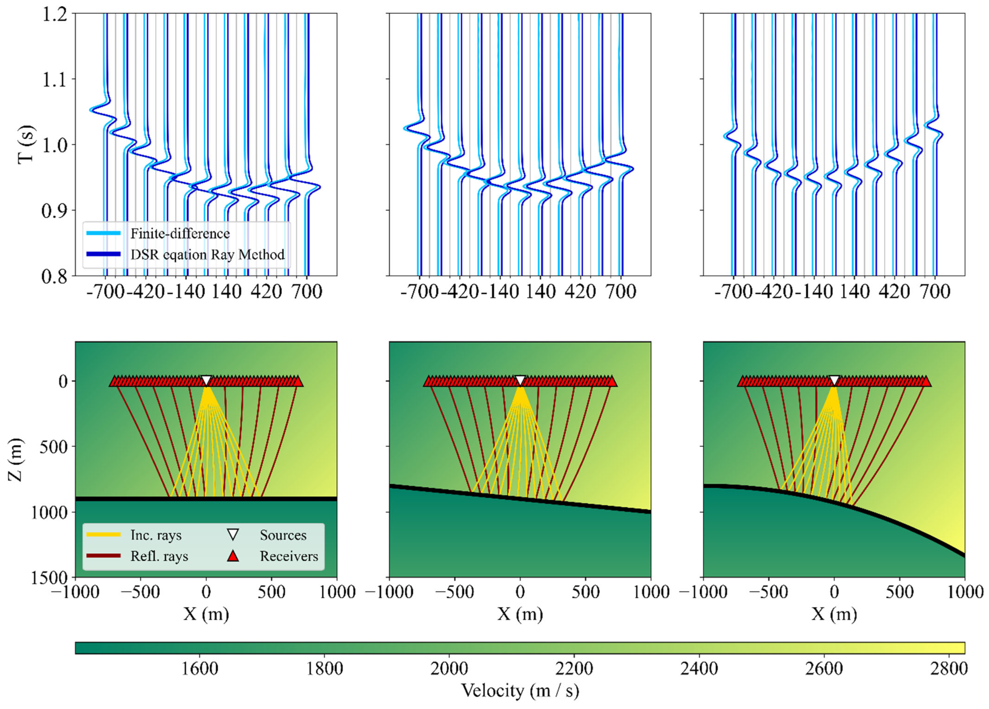
• Trace a family of DSR rays from the reflector to the surface using the Ray Tracing System (19) with initial conditions (31).
• Compute ray amplitudes using formula (43) and form synthetic seismograms using the technique presented in [18].
• Compare the DSR ray-synthetic seismograms with finite-difference wave equation gathers computed in the same model.
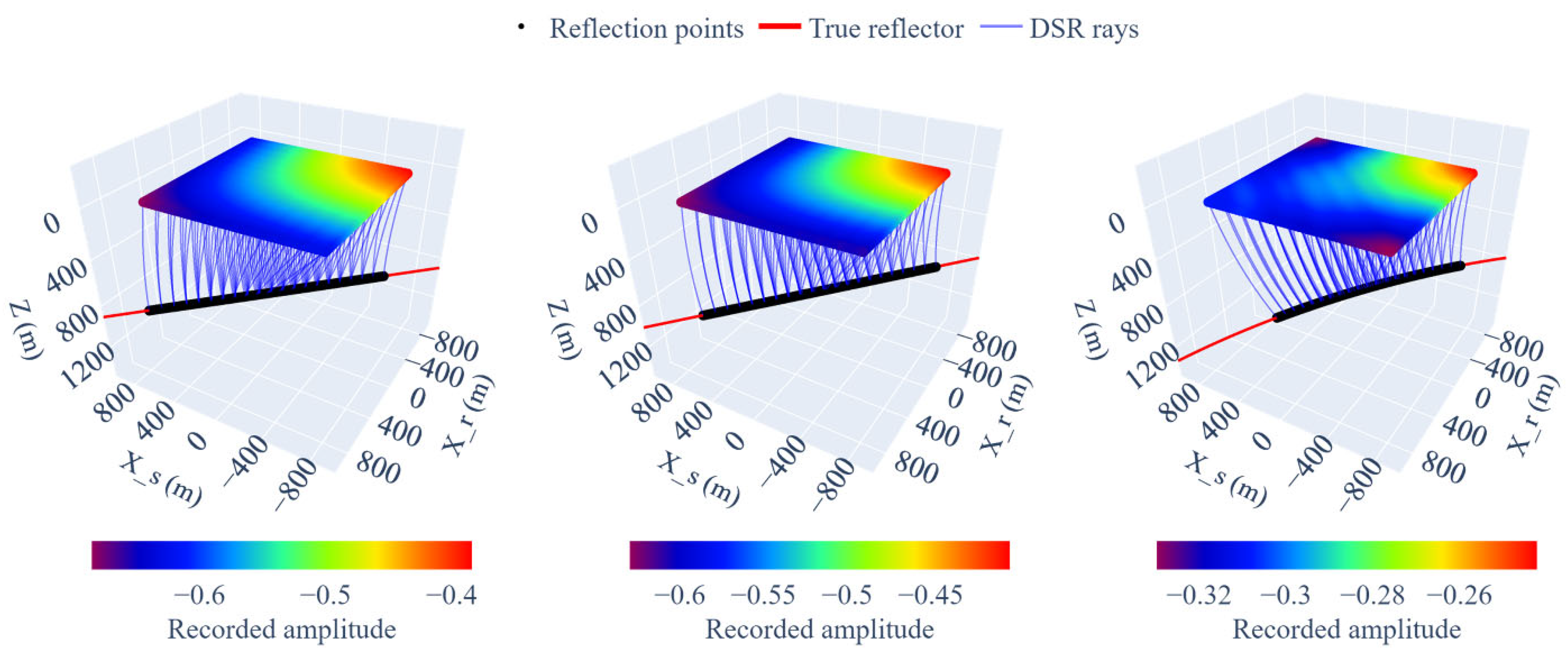
• Back-propagate the DSR rays from the survey plane down to the reflector using the Ray Tracing System (19) and initial conditions (35).
• Extract the reflectivities from the finite-difference data using formula (48) and compare them to the true ones.

In our experiments, we passed “true” travel time derivatives computed at the ray modeling step to the initial conditions (35), (36) when we back-propagated the wavefield. In a more realistic case, one ought to somehow estimate them from the recorded data. We shall briefly touch on this problem in the Discussion section below.

We consider three laterally varying velocity models given by

$$v\left(x,z\right)=\left\{\begin{array}{c}2000+\frac{x}{2\sqrt{2}}+\frac{z}{2\sqrt{2}}\hspace{1em}\left[m/s\right],\hspace{1em}z\le f\left(x\right),\\ 1000+\frac{z}{2}\hspace{1em}\left[m/s\right],\hspace{1em}z>f\left(x\right),\end{array}\right.$$

(49)

and differing in the reflector’s shape $f\left(x\right)$. We consider a horizontal reflector, a dipping reflector, and a curvilinear reflector:

$$f\left(x\right)=\left[\begin{array}{c}900\hspace{1em}\left[m\right],\\ \hspace{1em}900+\frac{x}{10}\hspace{1em}\left[m\right],\\ 4800-\sqrt{{4000}^2-{\left(x+1000\right)}^2}\hspace{1em}\left[m\right].\end{array}\right.$$

(50)

In all three models, the overburden velocity is greater than that of the bedrock, which precludes critical incidents where the standard ray method fails. There are no caustic regions in these models, which also favors ray method’s validity. All the models are shown in Figure 2.

We set up a survey consisting of $51$ sources and $51$ receivers ranging from $x=-700$ m up to $x=700$ m with step of $28$ m at zero depth. To trace the rays, we used the shooting method, iteratively searching for an appropriate reflection point and angle to hit the desired source–receiver pair. In the lower row of Figure 3, we show examples of common-shot ray diagrams. Evidently, our rays satisfy Snell’s law, and they are curved in the direction of the velocity gradient, which is in accordance with the standard ray method.

Moreover, the DSR ray method’s travel time and dynamics also match the wave equation modeling, as illustrated in the upper row of Figure 3. In this figure, two sets of wiggle traces are plotted parallelly. The darker traces are the DSR equation’s ray method solutions, and the lighter traces are finite-difference solutions of the wave equation. The direct wave was muted before plotting.

The focusing of the back-propagated wavefield can be better illustrated in the 3D extended volume. In Figure 4, we present ray diagrams of the back-propagated wavefield. It can clearly be seen that the rays are focusing on the reflector $x_s=x_r=x_0$, $z=f\left(x_0\right)$ in all three cases.

We applied our true-amplitude recovery formula (48) to the finite-difference data and obtained partial reflectivity maps of the reflectors. These maps consist of scaled reflection coefficients covering the illuminated part of the interfaces. We normalized them, making the reflectivity in the survey’s center a unit, and compared them to their theoretical values. We present the results of true-amplitude recovery in Figure 5. We plotted the recovered reflectivities as 3D scatterplots superimposed on the true reflectivity maps in the “reflection point—reflection angle—depth” space. We outlined the illuminated area with red triangles. Evidently, the recovered reflectivity accurately matches the true one in all three models.

Though our numeric tests above are but “toy” examples, we designed them to highlight the validity of the developed formalism only, and we do not intend to address full-scale seismic processing challenges at this moment. Furthermore, we do not have access to any DSR equation solver and thus cannot compare the performance directly. However, scaling our ray tracing engine to more realistic 2D applications, we reached a performance as high as 15,000 DSR rays per second on a modern PC. We emphasize that we relied on a Python implementation, which is not the best choice from the perspective of performance, and significant improvements should be expected from more professional programs.

4. Discussion and Conclusions

In our paper, we applied an asymptotic ray method approach to the true-amplitude Double Square Root equation. First, we reproduced the DSR eikonal equation known from other publications. Then, we derived an original transport equation describing ray amplitudes of the DSR equation solutions. We applied Hamiltonian formalism to solve these two equations and derived formulae for ray tracing, data modeling, and inversion. On the one hand, our results give further validation to the idea that the considered true-amplitude DSR equation preserves the ray amplitudes of acoustic waves. On the other hand, they form the basis for the further implementation of amplitude-preserving imaging methods, Gaussian-beam construction, and velocity estimation techniques. These asymptotic methods have proven to be reliable tools, significantly reducing computational costs in the context of wavefield modeling and imaging [17,18]. We expect similar results for the DSR equation applied to seismic or acoustic data acquired by source–receiver arrays. For instance, we plan to address the slope tomography [26] application of the ray perturbation theory for scattering object localization together with the velocity model update.

All the limitations of the standard ray method also apply to our DSR equation asymptotics. The derived formulae are inapplicable in the vicinity of caustics and critical-incidence rays. However, we think that uniform asymptotics developed for these regions in the standard ray theory should have their analogs for the DSR equation. Another limitation of the parabolic equation approach is that we assume no wave propagation in the direction orthogonal to the chosen direction, which may be horizontal or vertical for ocean acoustics, sediment layer studies, or seismic studies. We believe that this assumption may be satisfied in moderately inhomogeneous media. In addition, this difficulty can be mitigated by introducing local curvilinear coordinates where the waves will not turn to the undesired direction [27].

Note that for our asymptotic formulas, we need travel times and their derivatives as input for data back-propagation and true-amplitude recovery. Wave arrival travel times and their slopes are routinely estimated in the slope tomography method, and several techniques have been developed to extract them from seismic data [26,28,29]. Estimating the travel time second derivatives will require some extra work, but theoretically, they can be found by the slant stacking technique described in [30].

References

1. Jensen, F.B.; Kuperman, W.A.; Porter, M.B.; Schmidt, H. Computational Ocean Acoustics, 2nd ed.; Springer: New York, NY, USA, 2011; ISBN 978-1-4419-8677-1. [Google Scholar]
2. Claerbout, J.F. Imaging the Earth’s Interior; Blackwell Scientific Publications: Oxford, UK, 1985. [Google Scholar]
3. Makarov, D.V.; Petrov, P.S. Full Reconstruction of Acoustic Wavefields by Means of Pointwise Measurements. Wave Motion 2022, 115, 103084. [Google Scholar] [CrossRef]
4. Bleistein, N.; Cohen, J.K.; Stockwell, J.W.J. Mathematics of Multidimensional Seismic Imaging, Migration, and Inversion; Springer: New York, NY, USA, 2001; Volume 13, ISBN 978-1-4612-6514-6. [Google Scholar]
5. Biondi, B.L. 3D Seismic Imaging; Society of Exploration Geophysicists: Tulsa, OK, USA, 2006; ISBN 978-1-56080-137-5. [Google Scholar]
6. Roux, P.; Kuperman, W.A.; Hodgkiss, W.; Chun, H.; Akal, T.; Stevenson, M. A Nonreciprocal Implementation of Time Reversal in the Ocean. J. Acoust. Soc. Am. 2004, 116, 1009–1015. [Google Scholar] [CrossRef]
7. Belonosova, A.V.; Alekseev, A.S. On one formulation of the inverse kinematic seismic problem for a two-dimensional inhomogeneous medium. In Some Methods and Algorithms for Interpreting Geophysical Data; Nauka: Moscow, Russia, 1967; pp. 137–154. (In Russian) [Google Scholar]
8. Stolk, C.C.; Symes, W.W. Kinematic Artifacts in Prestack Depth Migration. Geophysics 2004, 69, 562–575. [Google Scholar] [CrossRef]
9. Alkhalifah, T.; Fomel, S.; Wu, Z. Source–Receiver Two-Way Wave Extrapolation for Prestack Exploding-Reflector Modelling and Migration. Geophys. Prospect. 2014, 63, 23–34. [Google Scholar] [CrossRef]
10. Zhang, Y.; Zhang, G.; Bleistein, N. True Amplitude Wave Equation Migration Arising from True Amplitude One-Way Wave Equations. Inverse Probl. 2003, 19, 1113–1138. [Google Scholar] [CrossRef]
11. Zhang, Y.; Xu, S.; Zhang, G.; Bleistein, N. How to Obtain True Amplitude Common-angle Gathers from One-way Wave Equation Migration? In SEG Technical Program Expanded Abstracts; Society of Exploration Geophysicists: Houston, TX, USA, 2005; pp. 1021–1024. [Google Scholar]
12. Zhang, Y.; Xu, S.; Bleistein, N.; Zhang, G. True-Amplitude, Angle-Domain, Common-Image Gathers from One-Way Wave-Equation Migrations. Geophysics 2007, 72, S49–S58. [Google Scholar] [CrossRef]
13. Cao, J.; Wu, R.S. Lateral Velocity Variation Related Correction in Asymptotic True-Amplitude One-Way Propagators. In SEG Technical Program Expanded Abstracts; Society of Exploration Geophysicists: Houston, TX, USA, 2009; Volume 28, pp. 2687–2691. [Google Scholar] [CrossRef]
14. You, J.; Wu, R.S.; Liu, X. One-Way True-Amplitude Migration Using Matrix Decomposition. Geophysics 2018, 83, S387–S398. [Google Scholar] [CrossRef]
15. Wu, C.; Feng, B.; Wang, H.; Wang, T. Three-Dimensional Angle-Domain Double-Square-Root Migration in VTI Media for the Large-Scale Wide-Azimuth Seismic Data. Acta Geophys. 2020, 68, 1021–1037. [Google Scholar] [CrossRef]
16. Khoury, A.; Symes, W.; Williamson, P.; Shen, P. DSR Migration Velocity Analysis by Differential Semblance Optimization. In SEG Technical Program Expanded Abstracts; Society of Exploration Geophysicists: Houston, TX, USA, 2006; pp. 2450–2454. [Google Scholar]
17. Popov, M.M. Ray Theory and Gaussian Beam Method for Geophysicists; EDUFBA: Salvador, Brazil, 2002; ISBN 8523202560. [Google Scholar]
18. Červený, V. Seismic Ray Theory; Cambridge University Press: Cambridge, UK, 2001; ISBN 9780521366717. [Google Scholar]
19. Duchkov, A.A.; De Hoop, M.V. Extended Isochron Rays in Prestack Depth (Map) Migration. Geophysics 2010, 75, S139–S150. [Google Scholar] [CrossRef]
20. Wolfram Research Inc. Mathematica, Version 13.2.0; Wolfram Research: Champaign, IL, USA, 2023.
21. Fomel, S.; Sava, P.; Vlad, I.; Liu, Y.; Bashkardin, V. Madagascar: Open-Source Software Project for Multidimensional Data Analysis and Reproducible Computational Experiments. J. Open Res. Softw. 2013, 1, e8. [Google Scholar] [CrossRef]
22. Harris, C.R.; Millman, K.J.; van der Walt, S.J.; Gommers, R.; Virtanen, P.; Cournapeau, D.; Wieser, E.; Taylor, J.; Berg, S.; Smith, N.J.; et al. Array Programming with NumPy. Nature 2020, 585, 357–362. [Google Scholar] [CrossRef]
23. Virtanen, P.; Gommers, R.; Oliphant, T.E.; Haberland, M.; Reddy, T.; Cournapeau, D.; Burovski, E.; Peterson, P.; Weckesser, W.; Bright, J.; et al. SciPy 1.0: Fundamental Algorithms for Scientific Computing in Python. Nat. Methods 2020, 17, 261–272. [Google Scholar] [CrossRef]
24. Hunter, J.D. Matplotlib: A 2D Graphics Environment. Comput. Sci. Eng. 2007, 9, 90–95. [Google Scholar] [CrossRef]
25. Plotly Technologies Inc. Collaborative Data Science; Plotly Technologies Inc.: Montreal, QC, Canada, 2015. [Google Scholar]
26. Lambaré, G. Stereotomography. Geophysics 2008, 73, VE25–VE34. [Google Scholar] [CrossRef]
27. Stolk, C.C.; de Hoop, M.V.; Symes, W.W. Kinematics of Shot-Geophone Migration. Geophysics 2009, 74, WCA19–WCA34. [Google Scholar] [CrossRef]
28. Schleicher, J.; Costa, J.C.; Santos, L.T.; Novais, A.; Tygel, M. On the Estimation of Local Slopes. In SEG Technical Program Expanded Abstracts; Society of Exploration Geophysicists: Houston, TX, USA, 2008; pp. 2998–3002. [Google Scholar]
29. Kai, X.; Yang, K.; Wang, Y.-X. Extracting a High-Quality Data Space for Stereo-Tomography Based on a 3D Structure Tensor Algorithm and Kinematic de-Migration. J. Geophys. Eng. 2017, 14, 792–801. [Google Scholar] [CrossRef]
30. Billette, F.; Le Bégat, S.; Podvin, P.; Lambaré, G. Practical Aspects and Applications of 2D Stereotomography. Geophysics 2003, 68, 1008–1021. [Google Scholar] [CrossRef]
Figure 1. Ray diagram of a reflection event.
Jmse 12 00636 g001
Figure 2. Velocity models. The black lines denote the reflectors’ position.
Jmse 12 00636 g002
Figure 3. Upper row: common-shot gathers. Darker lines correspond to the DSR equation ray modeling; lighter lines correspond to finite-difference wave equation modeling. Lower row: common-shot ray diagrams.
Jmse 12 00636 g003
Figure 4. Ray diagrams in the extended volume. Colored rectangles represent survey points and recorded amplitudes. The red lines mark the true interface position, the blue lines mark the DSR equation rays, and the black circles represent the reflection points.
Jmse 12 00636 g004
Figure 5. Reflectivity maps of the reflectors. The red triangles outline the scatterplots of the recovered reflectivity, while the background surfaces represent true reflectivity.
Jmse 12 00636 g005
Disclaimer/Publisher’s Note: The statements, opinions and data contained in all publications are solely those of the individual author(s) and contributor(s) and not of MDPI and/or the editor(s). MDPI and/or the editor(s) disclaim responsibility for any injury to people or property resulting from any ideas, methods, instructions or products referred to in the content.