1. Introduction
Currently, the role of autonomous underwater vehicles (AUVs) in ocean research is gradually increasing [
1,
2]. As AUVs have to operate far away from control centers at depths of tens or even hundreds of meters [
3], in many cases, it is not appropriate to surface every time when positioning is necessary, and therefore, using GPS is impossible for this purpose. A promising solution for positioning such AUVs is a long-range acoustic navigation system, consisting of navigation signal sources (NSS) deployed near the continental shelf zone and a receiver of such signals included in the vehicle hardware [
2,
4,
5].
Assuming that the NSS and the AUV have clock synchronization and the transmission time is encoded into the navigation signal, one positioning problem can be decomposed into several ranging problems (i.e., an AUV has to estimate its distance from several NSSs) and trilateration to identify coordinates [
6]. The widespread use of acoustics for ocean research began with the 1960 Perth to Bermuda experiment. This unique experiment led to the interesting idea of using acoustic signals at very large distances in the ocean to measure small changes in the average ocean temperature [
7]. Nevertheless, sound itself can be not only a means of research but also a carrier of information. Recently, acoustic experiments have been performed especially intensively [
8,
9,
10], including in the Arctic zone [
11,
12]. Sound propagation in the ocean occurs in a complex way with a number of effects, therefore, it is important to study the impact of these effects on the solutions of acoustic ranging problems. Thus, this paper is dedicated to the influence of an eddy on sound propagation in shallow-to-deep scenarios. The precision of the solutions of ranging problems depends on the completeness of the oceanographic information on the area of interest. To solve a ranging problem, one has to estimate the effective speed of sound propagation and, probably, also investigate to which extent its trajectory in the horizontal plane deviates from a geodesic line. Both the effective horizontal speed and the geometry are mostly affected by the bottom relief in a shallow sea and by sound speed spatial distribution. This distribution may be perturbed by different inhomogeneities such as internal waves [
13,
14,
15], temperature fronts [
16], and oceanic eddies [
17].
On the one hand, the presence of an anticyclonic eddy may result in an increase in the sound speed due to the local temperature perturbation [
16]. As a consequence, the signal could propagate faster than if there were no eddy. On the other hand, an eddy may deform the rays’ trajectories (horizontal eigenrays in the notation of [
18]), hence, the sound would propagate more slowly [
19]. With these two competing factors, a detailed study of the influence of an anticyclonic eddy on sound propagation is essential.
To take the presence of an eddy into account, the
field in the area between the source and the receiver is needed, e.g., within a certain strip on the earth’s surface along the acoustic track. Note that this field should be specified on a sufficiently fine spatial grid, such that all possible inhomogeneities are adequately represented. The hydrological measurements performed during the experiment are often sparse in time and space. Furthermore, the points where such measurements are carried out can be located not exactly on the trajectory of the sound propagation. In this study, we investigate the application of ocean circulation model data to the solution of a ranging problem. A variety of oceanographic reanalyses based on modern models such as NEMO [
20] or HYCOM [
21] provide a temporal and spatial resolution of the output data that cannot be achieved by performing measurements (e.g., [
19]).
Data obtained from ocean circulation models are used here for tracing horizontal rays [
22] and estimating arrival times, taking into account the three-dimensional geometry of sound propagation [
18]. After that, the estimated arrival times of modal components of the signal are juxtaposed with the impulse response function obtained in the experiment. Note that similar estimates can be performed assuming that sound propagates from the source to the receiver along the geodesic [
23]. Obviously, this latter approach can be reasonably accurate only if the horizontal refraction [
24] of sound is negligible. The influence of this phenomenon was discussed in [
24], where experimental data from an acoustic track aligned along the continental shelf break was analyzed.
The length of the acoustic path in the experiment analyzed in this study is about 1000 km. Less than 10% of the path length is shallow water (and the path is aligned approximately along the depth gradient). Thus, this scenario can be favorable for investigating the horizontal refraction caused by the presence of a synoptic eddy on a track. Indeed, bottom-relief inhomogeneities, e.g., the bottom slope (for example, 0.02° across-track and 0.05° along-track direction) that usually cause stronger horizontal refraction (that can obscure the more subtle effect of an eddy), are not expected to play a significant role in this case.
This paper is divided into seven sections and is organized in the following way. In
Section 2, the experimental data and satellite data are described. An explanation of some features of the models’ data and an anticyclonic eddy is presented in
Section 3. In
Section 4,
fields obtained from ocean circulation models are described, and the representation of the problem solution technique in terms of normal modes theory is given. In
Section 5, the horizontal eigenray calculations are described. In
Section 6, the influence of an eddy on sound propagation is estimated. Furthermore, this section is dedicated to the main results, in particular to a comparison of theoretical estimates of modal components’ arrival times with experimental data. In the Conclusions (
Section 7), the results are summarized and the perspectives of the method described below are discussed.
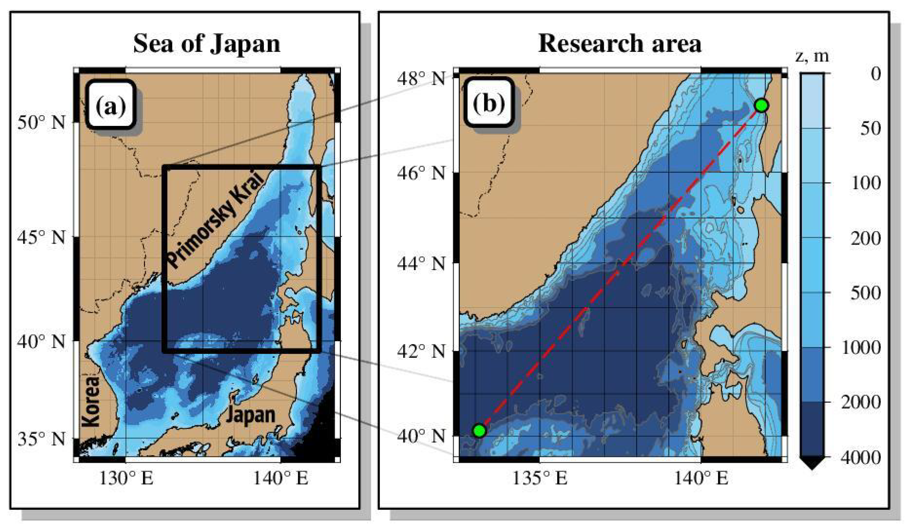
2. Experimental Area
The experiment discussed in this study [
25] was performed in August 2022 according to the scheme presented in general and detailed views in
Figure 1a and
Figure 1b, respectively.
An NSS was located at a depth of 39 m on the shelf near the Chekhov village (Sakhalin island) and the receiver was deployed from the research vessel at a distance of 1073 km from the source in the central part of the Sea of Japan near the Yamato Bank.
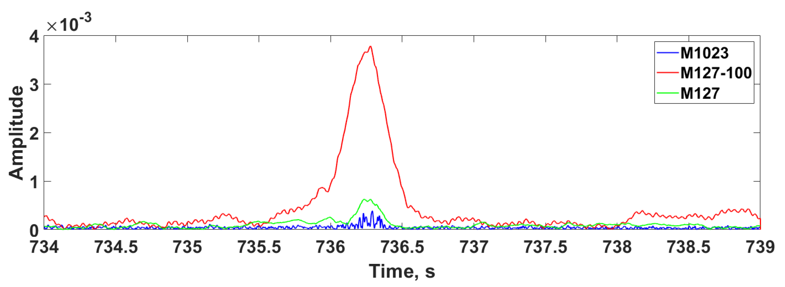
Every 6 min a signal consisting of several phase-shift keyed pseudo-random M-sequences with a carrier frequency of 400 Hz and the parameters specified in
Table 1 was transmitted, and impulse response functions (IRFs), shown in
Figure 2, were obtained.
To perform a theoretical estimation of the arrival times and effective velocities (see
Section 4) it is necessary to have the information about the sound speed distribution in the water column. During the experiment, the vertical profiles of temperature, salinity, and sound speed were obtained using direct CTD measurements near the receiving system and at three other points along the track. Obviously, such sparse experimental data does not give us full information about
in the area of interest. For example, since the distance between measurement points is hundreds of kilometers, a mesoscale eddy with a diameter of 100 km can be easily overlooked. Inhomogeneities in the sound speed field caused by such eddies may substantially affect sound propagation, thus, the investigation of related effects is important for the analysis of ranging/navigation systems’ performance.
It is usually the case that measurements cannot provide sufficient information about the field in the case of long-range propagation, as performing measurements along a path of hundreds or even thousands of kilometers in a reasonable amount of time is not feasible.
It is, therefore, necessary to take a different approach. One can use the sound speed data obtained by some high-resolution ocean circulation model, whereas direct measurements can be used to check its consistency with the conditions of the particular experiment. However, before proceeding to the implementation of this approach (see
Section 3), we would like to see whether one can actually expect some interesting propagation phenomena to manifest in the considered scenario.
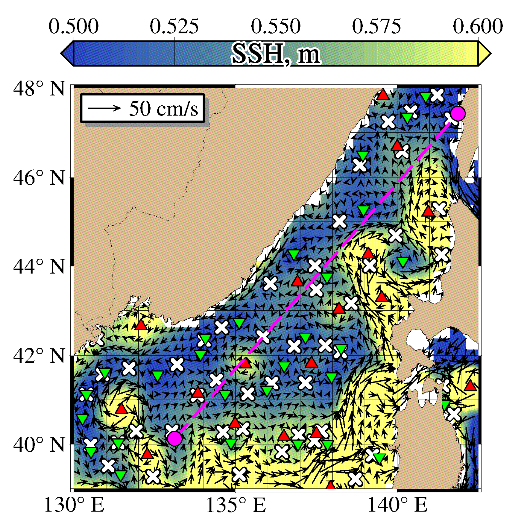
Some a priori analysis can be accomplished by using satellite altimetry data. This is a powerful method to investigate the ocean because the surface shape gives us certain information about the circulation under the sea surface. The processing of the sea surface height map (altimetry data) performed by AVISO (archiving, validation, and interpretation of satellite oceanographic data) provides the information about the water currents, as can be seen from
Figure 3.
In the considered experiment, the acoustical path is crossed by an anticyclonic eddy approximately at E. As an eddy was identified, the influence of this particular hydrodynamical feature will be discussed in the next section.
3. Oceanographic Reanalyses Data Usage
Reanalyses based on the ocean circulation models NEMO and HYCOM can provide high-resolution oceanographic data for long-range sound propagation modeling. The two models, however, feature important differences that can lead to both quantitative and qualitative discrepancies in simulation results. Firstly, the models use different types of vertical coordinates (hybrid coordinates for HYCOM and a combination of s- and z-coordinates for NEMO). Secondly, they use different atmospheric data sources and assimilation models.
Different reanalyses based on ocean circulation models may provide us with high-resolution oceanographic data with the assimilation of real oceanographic data. The quality and completeness of ocean parameters obtained from a reanalysis are higher than those obtained from a forecast made by the same circulation models due to the assimilation of oceanographic data for the period of interest in the former. Since ocean modeling techniques are being constantly improved, we expect that in the near future the circulation models will be capable of providing high-resolution forecast data on the temperature, salinity, and sound speed fields on the same level of accuracy as the present-day reanalyses. In our study, the reanalyses are used for theoretical predictions of the arrival times of pulse signals and for investigating the accuracy of such predictions in the case of using the most precise data available.
In this study, the data from the two oceanographic reanalyses, Global Ocean Forecasting System (GOFS 3.1), based on HYCOM [
21], and Copernicus Global
Oceanic and Sea Ice Reanalysis (GLORYS12) based on NEMO [
20], are used. Their main characteristics are given in
Table 2. The two models use different numerical schemes as well as different approaches for the modeling of certain physical processes in the ocean. In the reanalyses mentioned above, different sets of measurement data and assimilation methods are used. A convenient criterion for verification is the AVISO data. Although most oceanographic reanalyses assimilate the sea level from AVISO, they may still differ from it for a variety of reasons.
Identifying an eddy in the reanalysis data is a complicated problem since the oceanographic data (e.g., T/S fields) contain only certain signs of its presence, such as perturbation of temperature isolines. The oceanographic data should be processed using a special method to identify eddies and trace back their genesis. Lagrangian analysis is an advanced state-of-the-art tool that can be used for this purpose [
26]. It consists in tracking multiple Lagrangian particles moving along the streamlines of the current velocity field. This method allows the evolution of individual eddies to be followed in the output data fields of ocean circulation models.
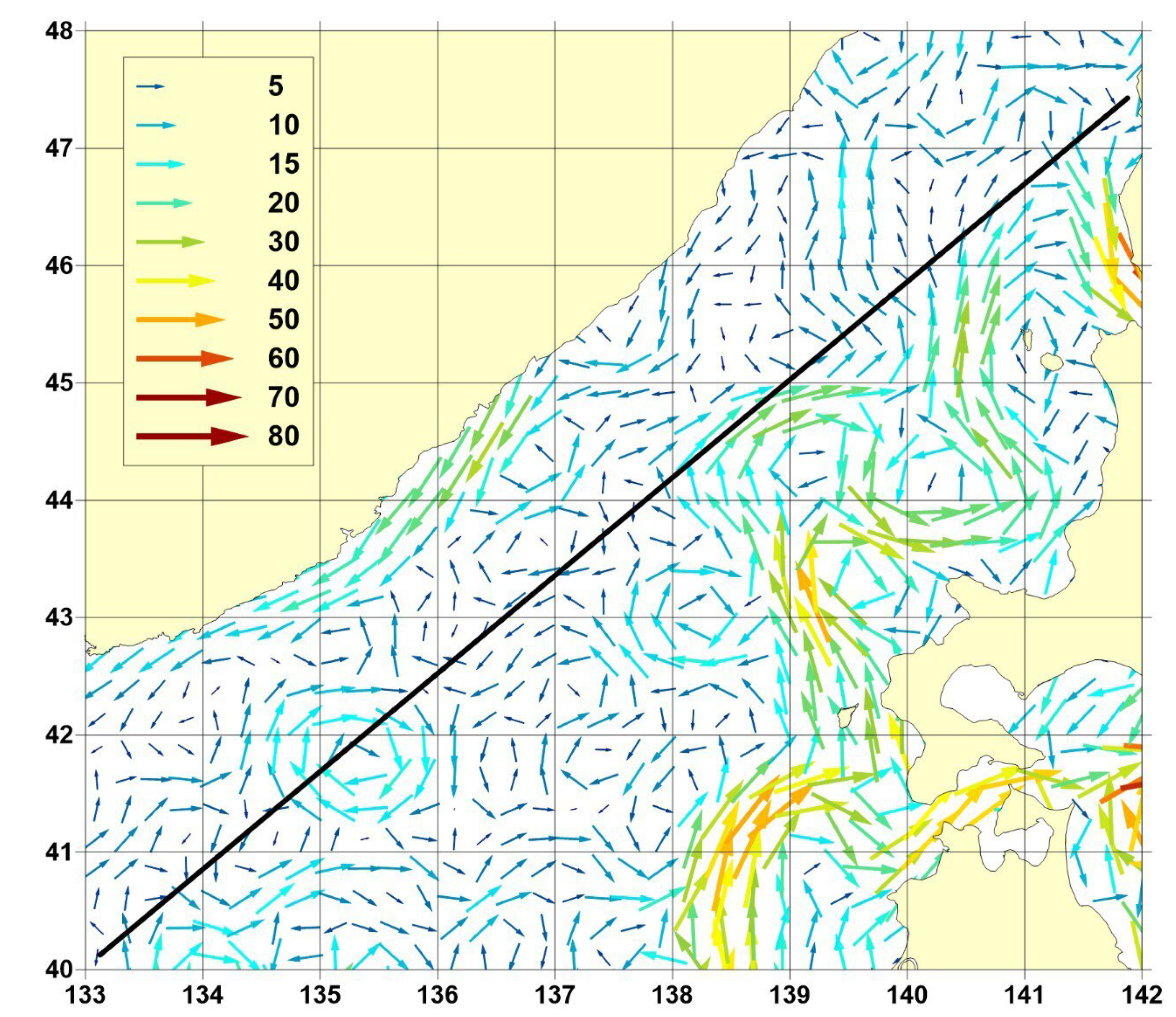
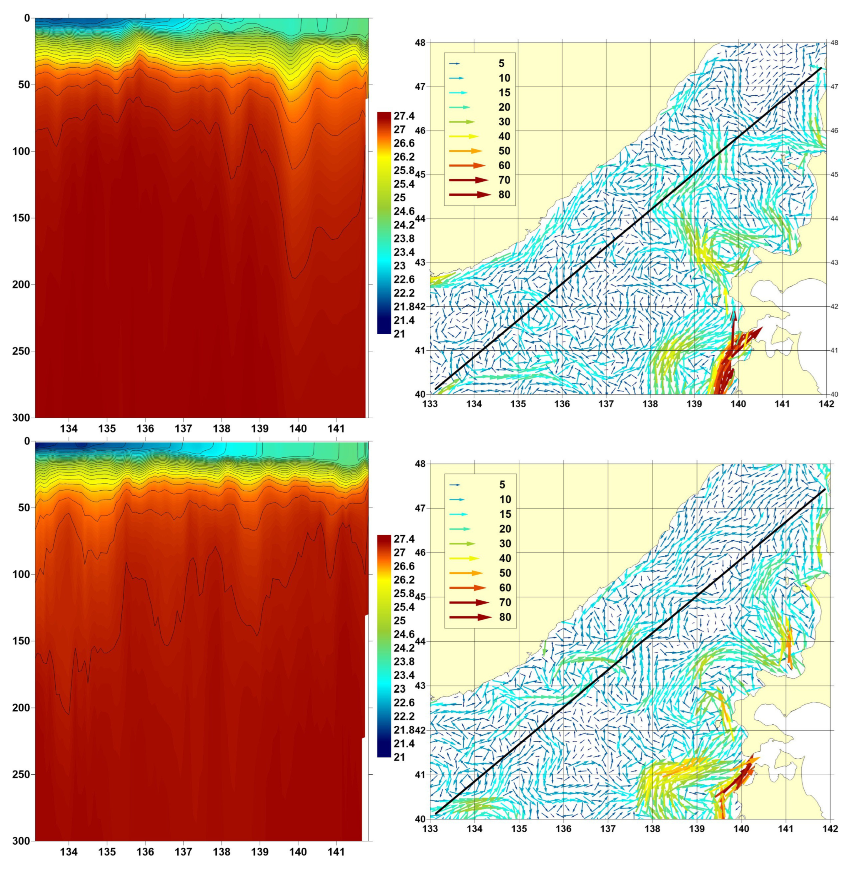
The Lagrangian analysis procedure can be summarized as follows. The density is calculated from temperature and salinity data taken from a reanalysis, then the currents are calculated from density data using a linear diagnostic model [
27]. This procedure is performed for different reanalyses, and the obtained currents are compared with the AVISO data (see
Figure 4 and
Figure 5). The reanalysis exhibiting the best agreement with the latter is selected for use in the Lagrangian analysis.
In this study, the circulation of the waters of the Sea of Japan in the area of the experiment is considered. The density field (as shown in
Figure 5) used for the diagnostic calculations is computed by using the seawater equation of state [
28] based on the temperature and salinity data obtained from the GOFS3.1 and GLORYS12V1 oceanographic reanalyses. The respective current velocity fields are also presented in
Figure 5. Visual comparison with the AVISO data in
Figure 4 shows that the GOFS3.1 reanalysis matches it noticeably better. In practice, we would use the aforementioned comparison to decide which forecast/reanalysis to use for computing the sound speed field
. In the next section, however, we use the data obtained from both reanalyses to see if the effects on sound propagation geometry and the delay times are substantially different for GOFS3.1 and GLORYS12V1.
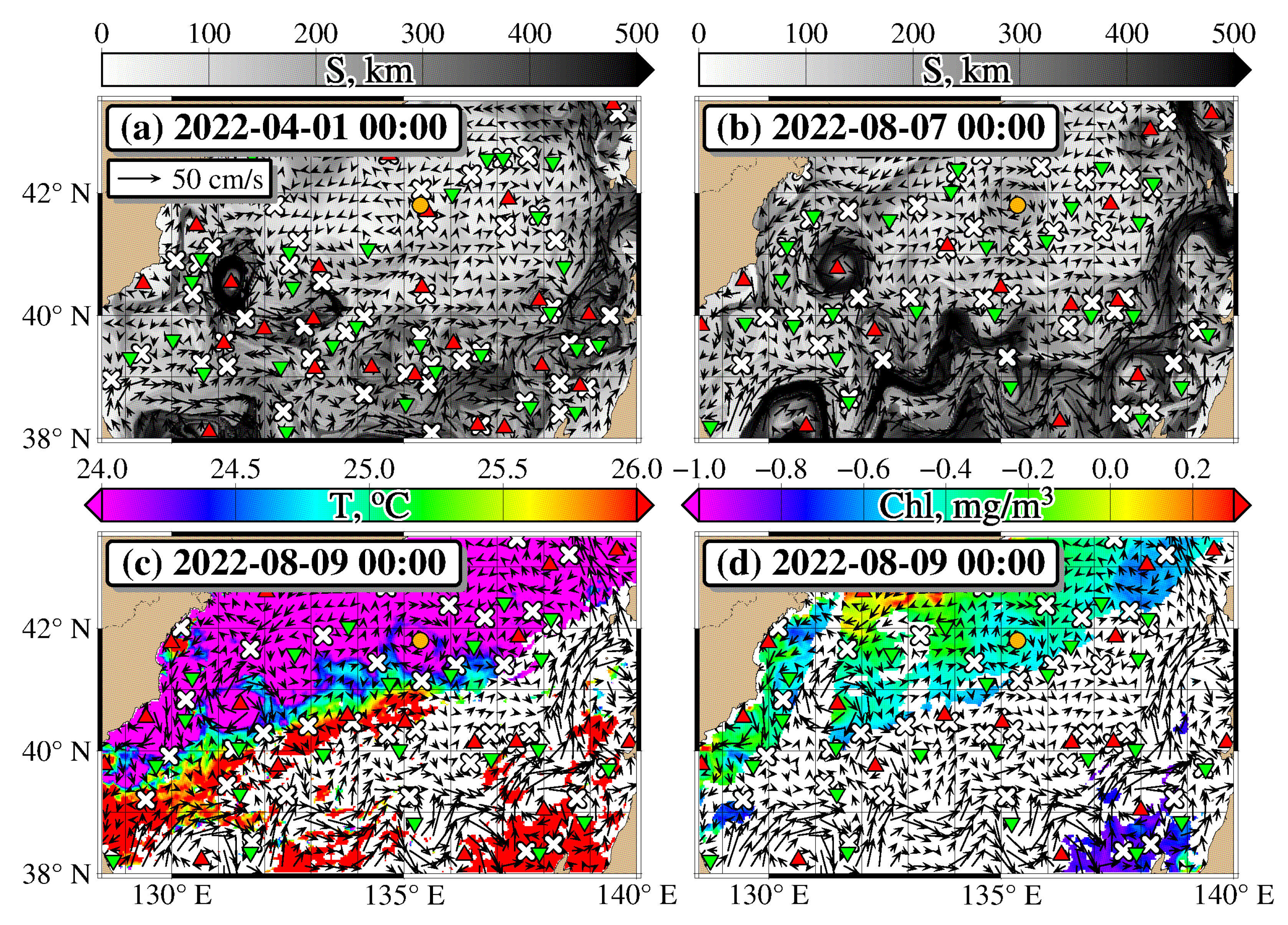
Based on AVISO, the Lagrangian analysis [
26] of mesoscale eddies in the area of the acoustic experiment was performed. The area of interest 38–48
N, 128–142
E was covered by a uniform 500 × 500 grid that was seeded with initial conditions every day from 1 April to 10 August 2022 (the experiment took place in the first half of August). The trajectories of passive particles starting at each grid point were back-propagated in time for 30 days.
The results of the tracing are shown in
Figure 6. The color bar in
Figure 6a,b encodes the value of the accumulated tracer’s trajectory length
S (in kilometers). The red and green triangles are the centers of anticyclones and cyclones, respectively, while the white crosses correspond to hyperbolic points of the current field [
29].
The mesoscale anticyclonic eddy that was observed in the experiment’s timeframe in the AVISO data can be seen on a series of Lagrangian
S-maps as well. The position of the eddy is marked by an orange circle at a point with the coordinates
N,
E in
Figure 6a,b. This eddy is accurately reproduced in the GOFS3.1 reanalysis (see
Figure 5).
According to the performed Lagrangian analysis, this eddy formed near the subarctic front around 1 April 2022 (red triangle with the coordinates 40
N, 133
E in
Figure 6) as a result of an intrusion from another anticyclonic eddy (see triangle with the coordinates 39.75
N, 132
E). Four months after its formation, the eddy was advected to the northeast and reached the area where the acoustic experiment took place.
Note that this eddy is also clearly seen on satellite images of ocean surface temperature (ST) and chlorophyll concentration according to MODIS Terra/Aqua satellite data, as shown in
Figure 6c,d. The eddy’s centers, obtained by means of Lagrangian analysis, are also superimposed onto these subplots to highlight their consistency.
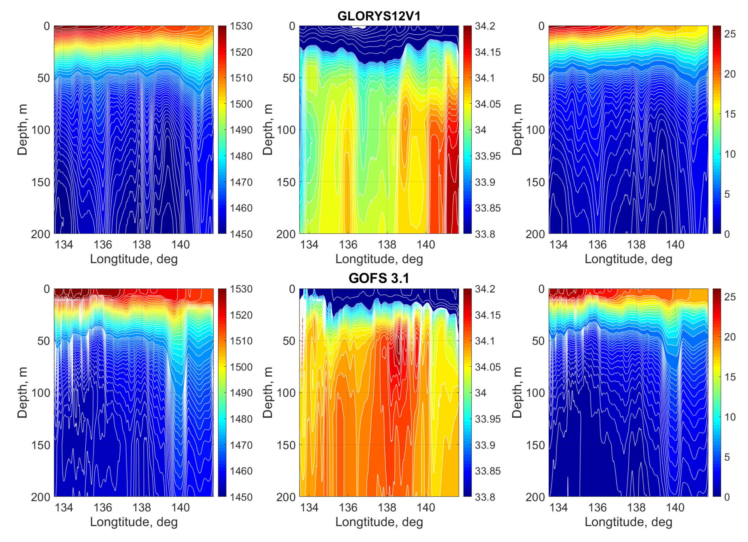
4. Model Data
As mentioned above, the vertical profiles of sound speed were obtained using direct CTD measurements near the receiving system and at the points at distances of 271.3, 404.3, and 652.5 km from the NSS along the path (
Figure 7).
For tracing the horizontal rays (i.e., to study the geometry of the modal components’ propagation) the information about
is needed not only along the acoustic path but also in some of its neighborhood [
1]. Modern oceanographic reanalyses, such as GOFS3.1 or GLORYS12V1, provide high-resolution data on temperature
, salinity
, and, as a consequence, on
. The field obtained from these models has a spatial resolution up to
, so it can represent large-scale (>100 km) and mesoscale (from 50 to 100 km) ocean inhomogeneities that can affect sound propagation. In the considered experiment, such inhomogeneities are also visible on cross-sections of salinity and temperature near
E, shown in
Figure 8.
Indeed, the noticeable divergence of the isolines of these parameters around E indicates the presence of an eddy. Clearly, the variation in the , and fields is also expected in the across-track direction.
As mentioned earlier, the influence of anticyclonic eddies on sound propagation is possible in the following two ways:
These two factors are competing in the sense that the first one leads to a decrease in the signal propagation time while the second one results in an increase. Below, we estimate the arrival times of the different modal components of the signal, taking both factors into account, using the following two-step algorithm.
The first step consists of the calculation of the spatial distributions of group velocities
and wavenumbers
using normal modes theory [
22], as described in detail below.
Acoustic field
may be represented in the form of a modal decomposition [
22]
where
are the coefficients of the expansion over eigenfunctions
of the following Sturm–Liouville problem
in a given vertical cross-section of the ocean (it can be defined by the range
r from the source or the horizontal coordinates
). In Equation (
2),
is the angular frequency,
is the density, and
is the sound speed profile at the given vertical cross-section of the ocean, which parametrically depends on
coordinates. The second line’s equalities are the boundary conditions for the eigenfunction as
and
, respectively (where
H is some lower boundary of the computational domain). The third and the fourth lines represent the continuity of the eigenfunction and its normal derivative across the water–bottom interface
. The time-domain counterparts of the quantities
in the expansion (
1) are called modal components of the acoustic signal. For a narrow frequency band, they can be associated with the vertical distribution of acoustic energy described by the mode function
computed at the central frequency
of the signal (in our case, the carrier frequency
). The modal component of the acoustic signal corresponding to the function
propagates in the horizontal plane with the group speed
Note that this quantity is computed for a given cross-section of the waveguide, i.e., parametrically depends on the range r (or, more precisely, on the horizontal coordinates ) and the frequency. For the signals considered in this study, the intermodal dispersion (i.e., the variance of the group velocities of a given mode within the frequency band of the signal) turns out to be negligible, and in what follows, are always computed for the central frequency .
In the second step the wavenumber distribution
is used to compute horizontal eigenrays (see
Section 5). The variations in
in the cross-track direction may result in so-called horizontal refraction that manifests in the deviation of eigenrays from the geodesic. A theoretical estimation of the travel time can be obtained by integrating
along the propagation path. If the azimuthal coupling is negligible and the propagation can be considered two-dimensional, the inverse group velocities to be integrated simply along the geodesic are
where
R is the actual distance between the NSS and the receiver on the Earth’s surface (that is, the distance along the geodesic). Each sound speed profile
, in this case, corresponds to a point with a range
r from the NSS.
If the environment is such that variations in the media parameters across the path are significant enough, the azimuthal coupling cannot be neglected anymore. In this case, the propagation path of the modal components of the signal must be associated with the respective horizontal eigenrays
, parameterized by their arclength
s. Thus, the arrival times of the modal components can be estimated theoretically by computing their integrals in the form:
where
S is the length of the eigenray corresponding to the
j-th mode. Sound speed profiles for solving (
2) and subsequently computing the group velocities
along the eigenray are obtained from the 3D sound speed distribution as
.
In contrast to the travel time estimation formulae (
3) and (
4), acoustic ranging and navigation problems consist in the estimation of
R based on the knowledge of
. For this purpose, one has to replace the integration of
over the path by the averaging of
. Then, the formula below can be used:
where the effective speed of the
j-th modal component is defined as the group speed averaged over the path
A similar formula can be written for averaging
along an eigenray, although in the latter case the left-hand side of Equation (
5) is equal to
rather than
R.
Assuming that the propagation path (no matter whether a geodesic or an eigenray) consists of
n intervals of equal length with the sound speed profiles specified at their endpoints, we can compute
by using the following formulae [
24]:
where
is the group speed averaged over the
i-th interval, and
,
are group velocities of the respective mode computed at its endpoints by solving the Sturm–Liouville problem (
2).
On the one hand, the influence of an eddy can manifest in the variability in . On the other hand, its presence may lead to a horizontal refraction resulting in a substantial difference between and R. The latter effect may manifest in a systematic range estimation error. In this study, we quantify this error in the particular experiment discussed above.
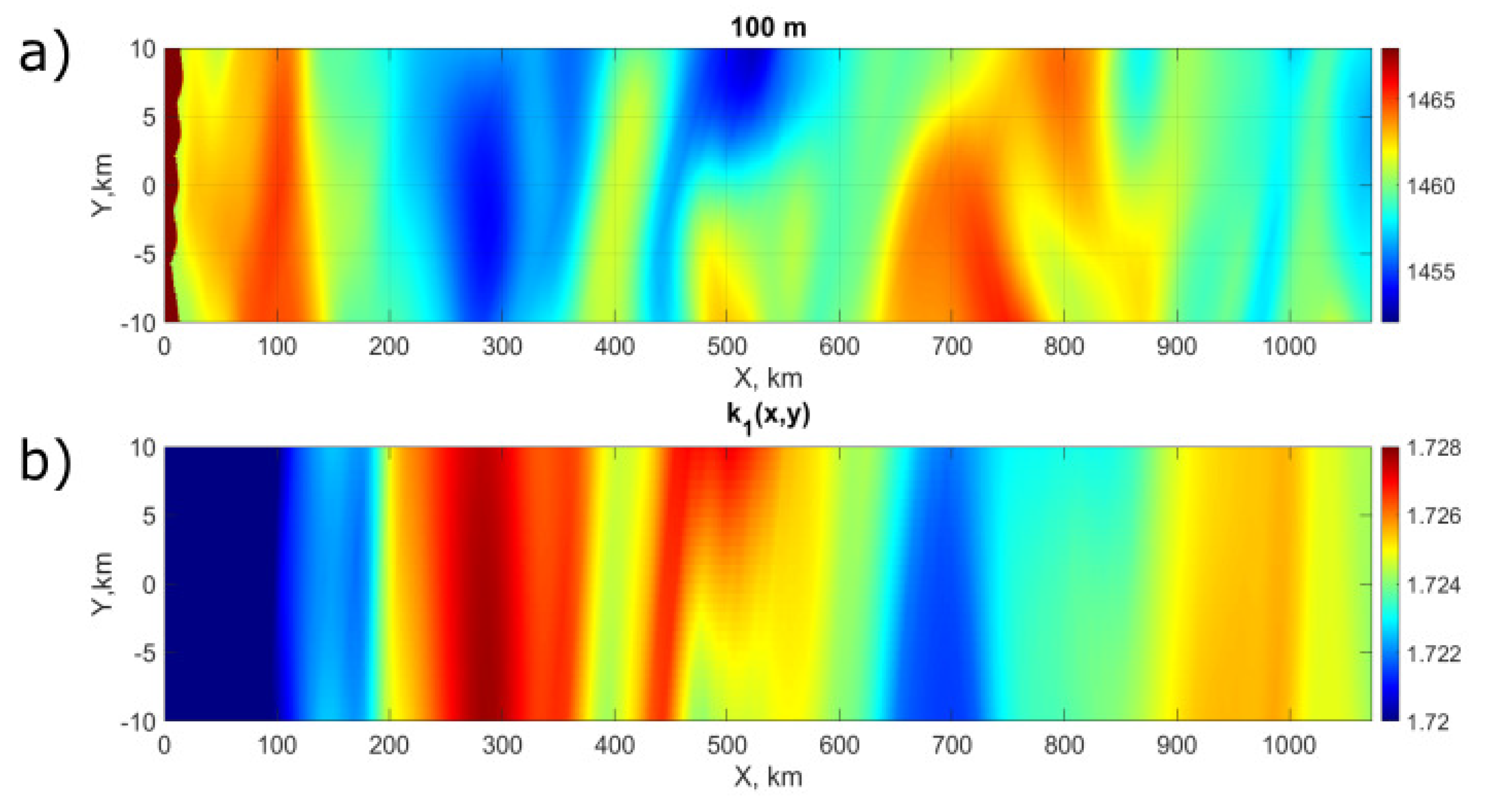
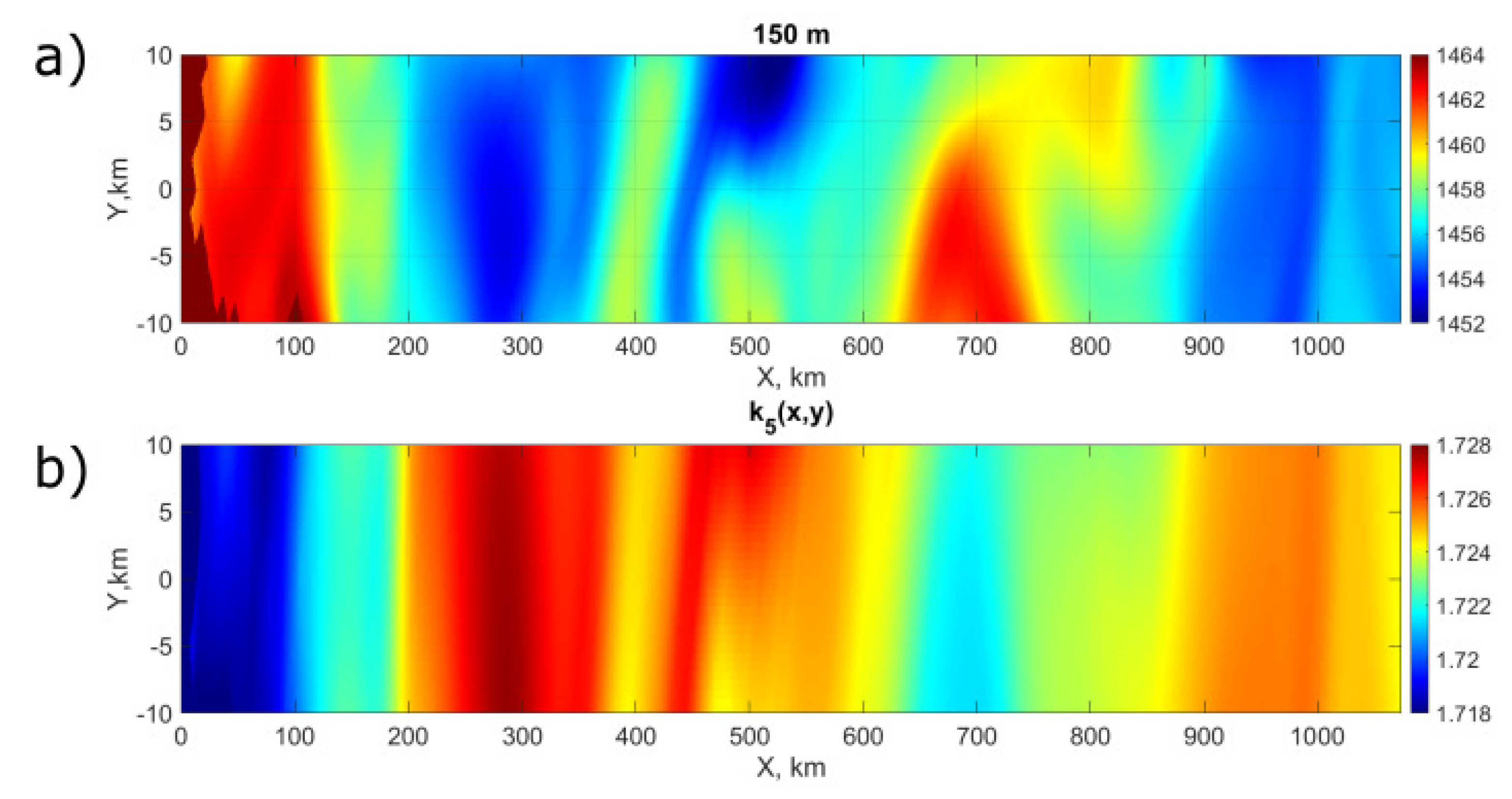
5. Fields of , , and Horizontal Rays
Let us introduce the Cartesian coordinates in the horizontal plane in such a way that the NSS is located at the point with coordinates and the receiver has coordinates (i.e., the Cartesian coordinate chart maps the source–receiver geodesic into the x-axis).
Computation of
and
are performed in a domain Ω that has the form of a stripe
of 20 km width containing the geodesic. Examples of the distribution of
are shown in
Figure 9 and
Figure 10 (for the modes of the order 1 and 5). In addition, in these figures, the distributions of
for some fixed values of
near the underwater sound channel axis are presented.
Note that the variation in sound speed in these cut-planes exhibits a strong correlation with the variation in horizontal wavenumbers
. In the presented coordinate system an anticyclonic eddy is located between
km and
km. The
field perturbations corresponding to this range interval are noticeable in the subplots
Figure 9a and
Figure 10a. The perturbations of
are characterized by relatively strong gradients (see
Figure 9b and
Figure 10b). These gradients are taken into account in the course of the horizontal ray computations [
30].
The horizontal rays are obtained by applying standard ray theory to mode amplitudes
satisfying the horizontal refraction equation [
22]. This approach was pioneered by Burridge and Weinberg [
18]. It can be shown that the horizontal ray trajectories [
31] can be computed as a 2D projection of the bicharacteristics satisfying the following Hamiltonian system
complemented with the following initial conditions
where
is the launching angle of a ray.
A solution of Equation (5) is a curve in four-dimensional phase space
called a bicharacteristic. Its projection
onto two-dimensional coordinate space is called a horizontal ray, corresponding to the
j-th mode component with starting angle
(this is a grazing launch angle with respect to the
x-axis). A ray connecting the source and the receiver is called an eigenray. As was mentioned above, we associate the propagation path of the
j-th modal component of the signal with the respective eigenray computed at the central frequency (note that horizontal rays depend on the frequency; however, within the context of the present study this dependence does not play an important role [
24]).
In order to identify the eigenrays for each mode (which is basically the same as identifying their respective launching angles
) we use the following algorithm. First, the solution of the system (5) should be obtained for a uniformly spaced set of launching angles within a certain interval
to obtain a fan of rays for each modal component. Assume that the receiver point
is located between two adjacent rays with the launching angles
, passing through the points (
) and (
). The eigenray grazing launch angle
can be estimated using the formula
which is very accurate provided that the step in the angle between adjacent rays is small (otherwise it can be used iteratively).
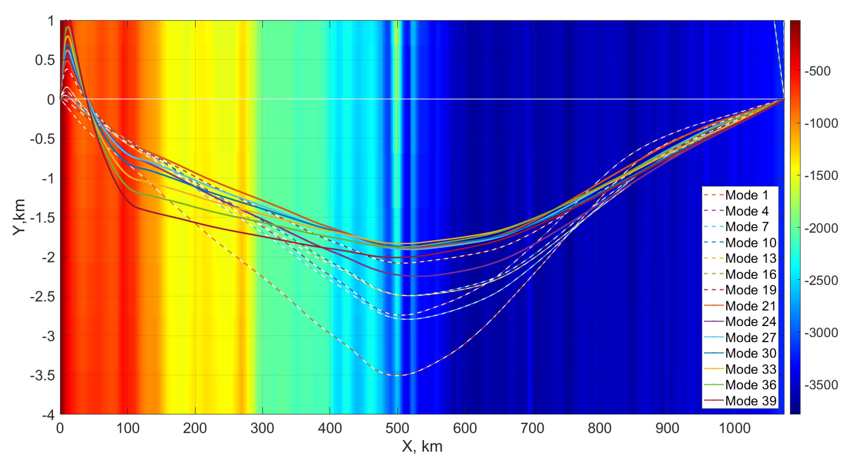
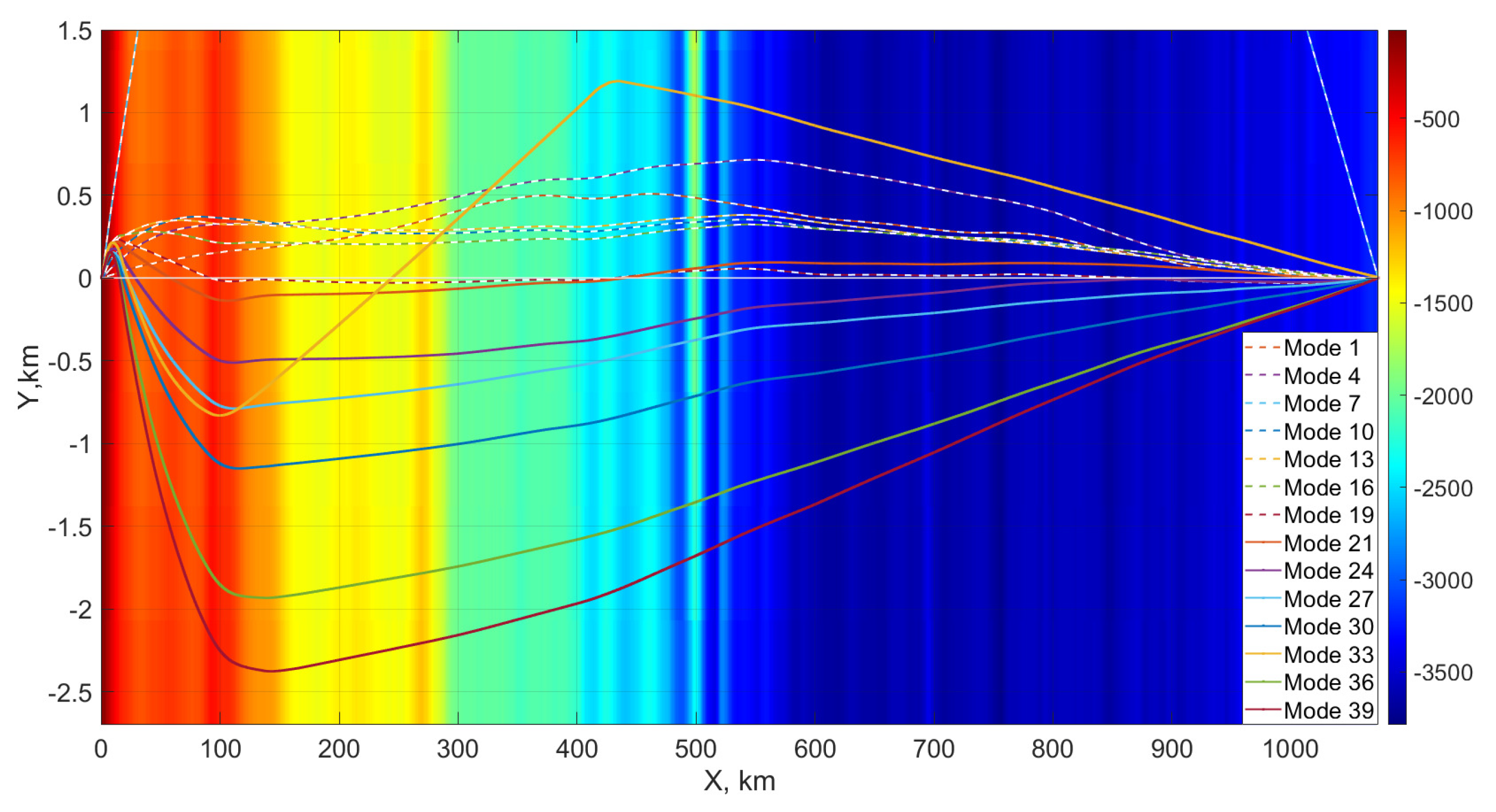
In
Figure 11 and
Figure 12, eigenrays calculated by using the sound speed distributions
from the GLORYS12V1 and GOFS3.1 oceanographic reanalyses, respectively, are presented.
In this study, the shallow-water part of the acoustic track is relatively short, therefore, horizontal refraction effects caused by the bottom-relief inhomogeneities can be expected to be relatively weak [
32], especially for low-order modes that correspond to the vertical rays with small grazing launch angles with respect to the underwater sound channel axis in the deep-water part of the path [
23]. However, as can be seen in
Figure 11 and
Figure 12, the curvature of horizontal eigenrays in the shallow-water part is much more pronounced than in the deep ocean, despite the presence of the eddy. This phenomenon takes place even in the case of a path aligned approximately across the bottom slope). Thus, we can conclude that even in our case the contribution of the horizontal refraction caused by the sound speed inhomogeneities is not significant. Its effect on the rays’ elongation is quantified in the next section.
6. Quantification of the Horizontal Refraction Influence
The deviation of horizontal eigenrays with length
from the geodesic with length
leads to its elongation
This value can be used as an estimation of the horizontal refraction influence and calculated using the formula above.
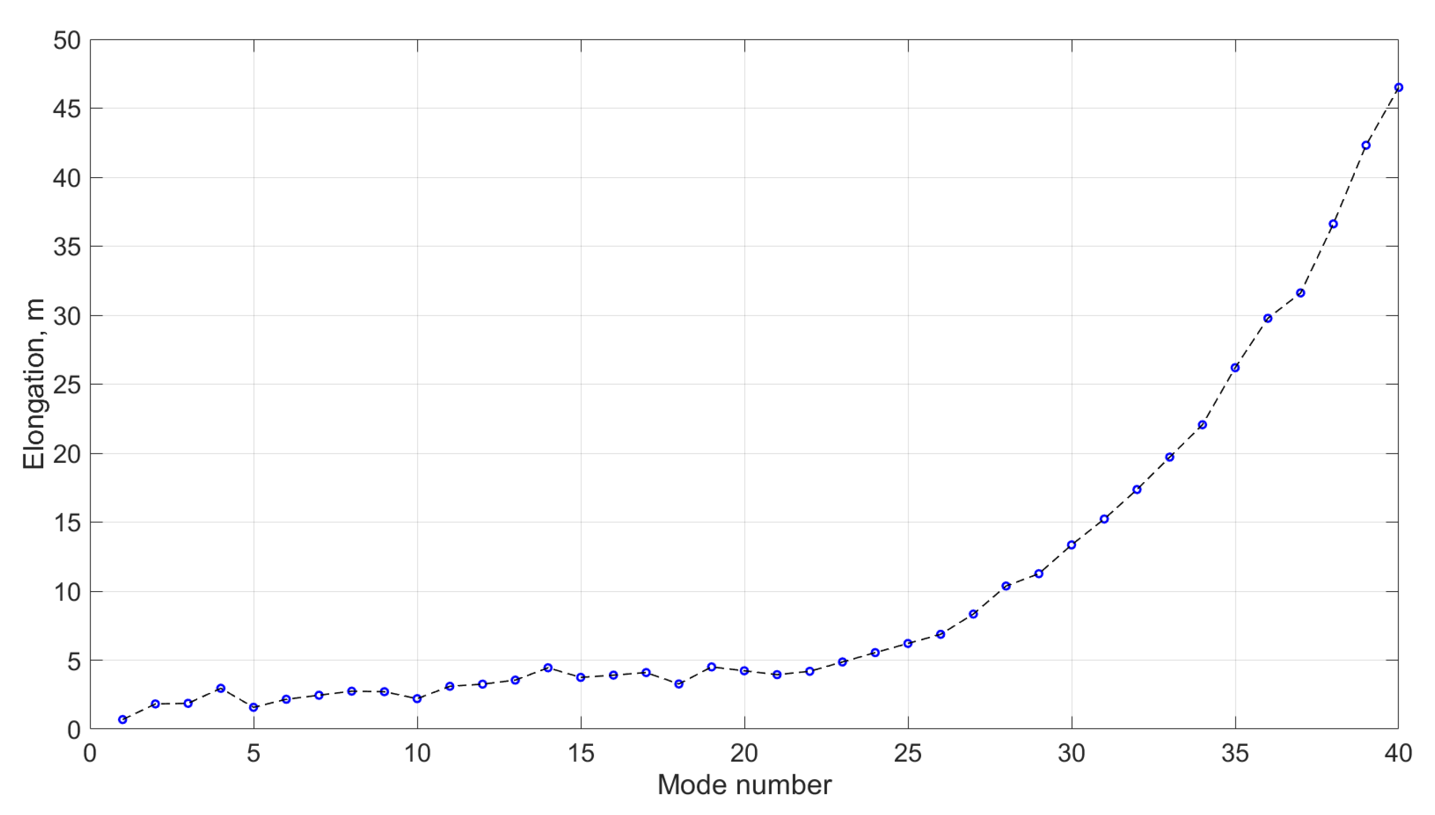
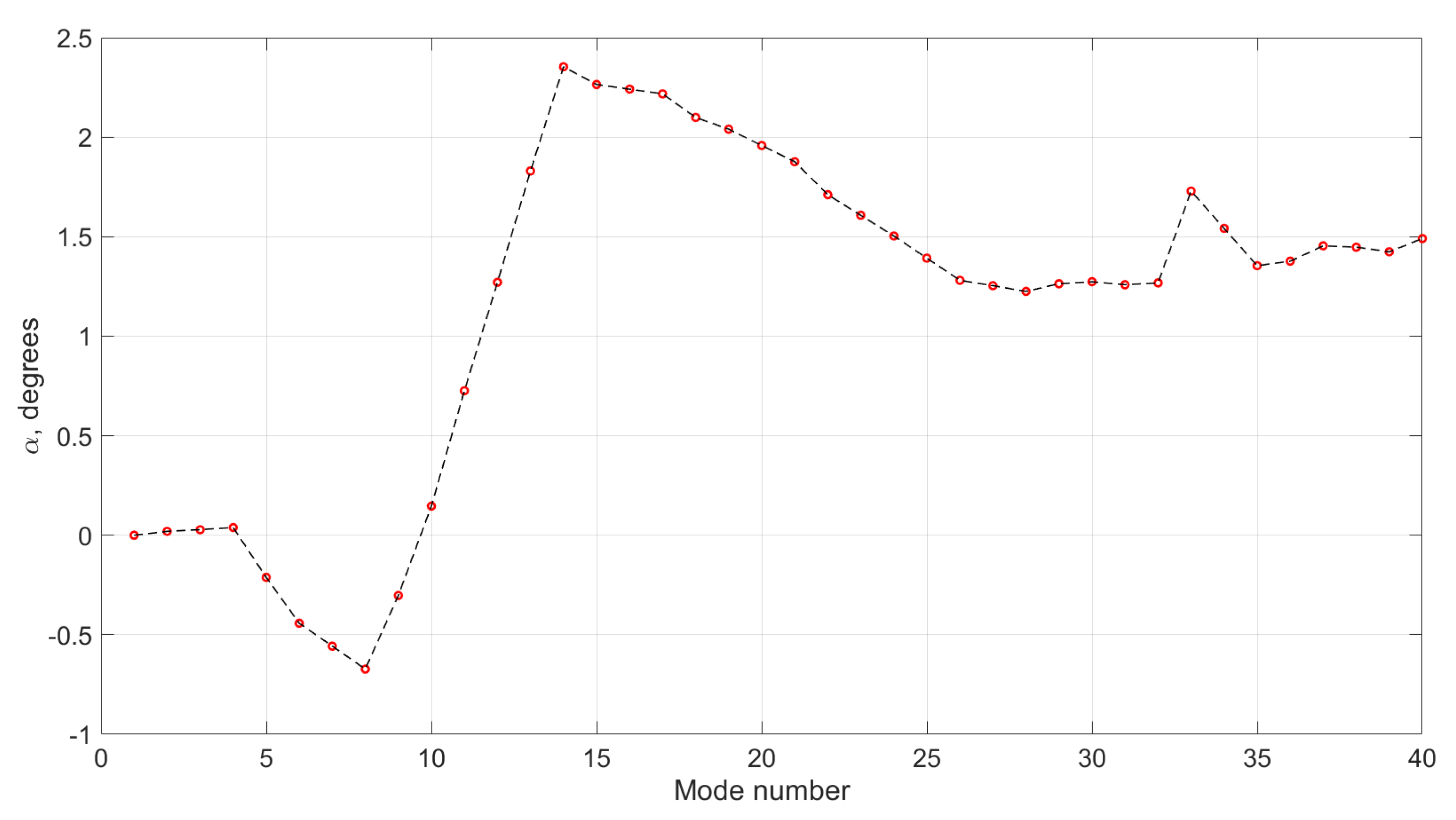
Further calculations are performed for the GOFS3.1 reanalysis. The elongations and grazing launch angles of the eigenrays are presented in
Figure 13 and
Figure 14, respectively. The eddy contribution to the horizontal refraction influence cannot be separated from the bottom-relief contribution. However, in quantitative terms, it is definitely even smaller than the values presented in
Figure 13.
Overall, the eigenrays in the case of the considered experiment are longer than the geodesic by a value from 0 to 50 m (depending on the mode number). Note that this is far less than was observed in [
24] for the 130 km path aligned along the shelf break, where the horizontal refraction on the sloping bottom plays a much more significant role.
As was shown above, horizontal refraction caused by an anticyclonic eddy leads to relatively small elongations of the propagation path as compared to the source–receiver distance (1073 km).
Let us now put together the formulae from
Section 5 and
Section 6 and estimate the arrival times of the modal components
by performing integration along the eigenrays according to Equation (
4). In principle, this is just an indirect way to evaluate the accuracy of the effective speed
estimation, and in the practical ranging/navigation problems, we would perform the computation of
R (or, more precisely,
) instead of using the measured
.
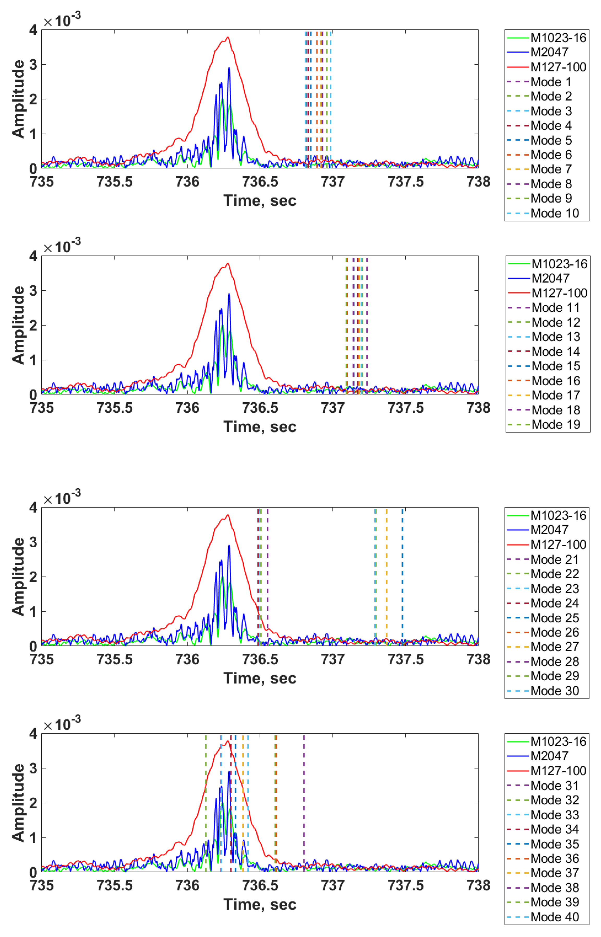
In
Figure 15, the IRF computed from the signals received in the experiment is presented together with arrival time marks corresponding to low-order modes. Note that for modes 1–10, the arrival time prediction error varies from 0.5 to 0.7 s, while for modes 11–20 it can be as large as 1 s. This would correspond to a range estimation error of approximately 800 m provided that we associate the peak in the M127-100 signal with the effective speed obtained by averaging
over the first 10 modes.
In previous works [
23,
24], the presence of a dense group of low-order modes is indicated. In this case, such groups are formed by modes 11–20 or 1–10 that are likely to form a weakly diverging beam in the underwater sound channel [
2,
33]. Such beams manifest in local maxima (determined by the intermodal dispersion) of IRFs corresponding to the aforementioned groups of waveguide modes. Their presence simplifies the problem of attributing mode numbers to the maxima of the observed IRF.
The discrepancy between the peaks in IRF and
may be explained in the following way. The part of the Sea of Japan where the experiment took place is an area with a relatively low concentration of ARGO buoys that perform real-time oceanographic measurements used by GLORYS12V1 or GOFS3.1 oceanographic reanalyses [
23]. Thus, ocean circulation models may give incomplete information about the sound speed field in the area of interest.
7. Conclusions
The correct theoretical estimate of the propagation speed of the modal components of an impulse acoustic signal is a key step in the solution of ranging problems. Successful estimations of these velocities depend on the completeness of both and the bathymetry data in the area of interest. The most promising source of information on the sound speed field is arguably the global ocean circulation models that provide high-resolution data on oceanographic parameters’ distributions (including ). In particular, this can be used for theoretical estimates of the arrival times of the modal components of a pulsed acoustic signal.
The practical implication for the method described in the presented study may be organized in the following way. The AUV uses fields of , calculated in advance (for example, based on ocean circulation models forecast data), because the spectral problem is a time-consuming process. Then, the hardware of the AUV is used to estimate the arrival times of the modal components. Such a way to organize the calculation may possibly be an example of the realization of the method described.
For a 1000 km long acoustic track in the Sea of Japan, the use of the sound speed data from the reanalyses based on the GOFS3.1 and GLORYS12V1 oceanographic reanalyses circulation models results in a ranging error of about 800 m. Although such accuracy still does not meet certain requirements on practical long-range navigation systems, it will be definitely improved in the near future with the advances in ocean circulation modeling.
Another important issue for the development of acoustic ranging systems is the effect of horizontal refraction. In deep-water propagation scenarios, this can be caused by the presence of oceanic eddies. Despite the strong cross-track variability in the sound speed field in the considered experiment, it is shown that horizontal eigenrays connecting the source and the receiver for the mode numbers from 1 to 40 are longer than a geodesic by no more than 50 m. Obviously, this contribution is negligible given the path length and the total ranging error. In particular, this fact highlights the robustness of long-range acoustic navigation systems to a horizontal refraction influence, except for the cases of nearly cross-slope propagation [
24].

 ,
, 


