Main Physical Processes Affecting the Residence Times of a Micro-Tidal Estuary

Abstract

Residence time is an important parameter linked to the water quality in an estuary. In this paper, we identify and analyze the main processes that affect the residence time of the Caloosahatchee River Estuary, a micro-tidal and mixed diurnal-semidiurnal estuary located in western Florida. Multiyear validated hydrodynamic hindcast results were coupled with an offline particle tracking model to compute the residence time of the estuary, which showed a strong seasonality driven by the river discharge. The residence time reduced with increasing river flow. The wind velocity and direction also affected the residence time. The influence of the wind was dependent on the magnitude of the river discharge. In general, upstream-directed wind increased residence time, while downstream-directed wind decreased residence time. Downstream wind during the dry period reduced residence time on average by a week. Processes such as water density gradient-induced circulation and particle buoyancy also influenced the residence time of the estuary. The outcomes of this study can be used to better understand the influence of the main physical processes affecting the residence time at other similar estuaries and to help in the management of the estuaries to improve their water quality.

1. Introduction

Estuaries are unique environments that are ecologically diverse and valuable systems worldwide [1]. They also support many economic and recreational services to the communities in these areas [2]. Increased human activities around estuaries can adversely affect these ecosystems’ water quality, usually by modifying the concentration of dissolved chemicals [3,4,5]. Apart from anthropogenic pressures, the water quality of an estuary also depends on the water circulation patterns and how rapidly different parts of the estuary can be “flushed” [4,6]. The flow patterns and the subtidal circulation in an estuary are governed by complex hydrodynamic interactions between coastal, fluvial, and atmospheric processes (e.g., [7]). Numerical modeling is commonly used to better understand the circulation patterns and ecological implications of estuarine environments [8].

Residence time in an estuary is defined as the time taken for a water parcel to leave the estuary. A higher residence time indicates that the estuary has less circulation and tends to retain nutrients, which can lead to water quality issues within the environment. Residence time is a commonly used parameter to discuss biogeochemical processes in estuaries [9,10]. Residence time can also provide information on the possibility of eutrophication [11], which may lead to adverse water quality issues due to phytoplankton blooms [12] and hypoxia [13].

Residence times depend, among other factors, on the morphological characteristics of an estuary [10]. For a given estuary, temporal variations in residence time also occur due to alterations in circulation patterns due to changes in processes such as tidal characteristics, riverine flows [14], wind fields [13], and barometric pressure [15].

The particle age is another important time scale that can be used to quantify the transport of matter in a system. The age provides information on how long particles remain within a given region [16]. The particle age has been used in previous studies to understand and quantify pollutant transport in coastal systems [17,18].

This study focuses on the residence time and the particle age in the Caloosahatchee River Estuary in Florida, United States (hereinafter referred to as CRE). Located on the west coast of the Florida peninsula, the CRE and Charlotte Harbor are vital areas for human and ecological activities. The CRE is connected to the Charlotte Harbor Estuary and spans a total area of ~800 km², which makes it the second-largest estuarine system in Florida [19]. The CRE is 42 km in length, spanning from Franklin Lock and Dam (S-79) to Shell Point [20]. The estuarine width ranges from 160 m at the upstream end to 2500 m downstream. The main channel of the estuary is ~5 m deep from Beautiful Island to Shell Point (Figure 1a and Figure 2).

The CRE is connected to Lake Okeechobee by the Caloosahatchee River via a series of dams and canals. The freshwater flow to the estuary is highly regulated and varies over the year. The tides are mixed diurnal-semidiurnal and micro-tidal, with an average tidal range of 0.8 m in the lower part of the estuary. Due to the variations in freshwater flow to the estuary, the salinity structure (length of salinity intrusion through the estuary, stratification) shows significant changes over time [21,22].

The CRE has been mired in water quality issues for decades [23]. Water quality in an estuary is directly influenced by physical forcings (e.g., freshwater discharge and wind forcings) [24]. The physical forcings impact the water quality by altering the fluxes and concentrations of different chemical constituents (e.g., dissolved oxygen, Total Nitrogen-n, Total Organic Carbon) and changing the residence time of the estuary [25].

The effect of Caloosahatchee River discharge on the concentration of chemical constituents has been investigated in many previous studies [26,27,28,29]. For example, the effect of river discharge on water quality parameters (e.g., Ammonia-n ($\mathrm{N}{\mathrm{H}}_4$) Nitrates, Ortho Phosphate-p, Total Nitrogen-n, and Total Organic Carbon) [26], phytoplankton communities [27], bottom dissolved oxygen concentration [28], and colored dissolved organic matter [29] has been extensively studied. The research by Xia et al. (2010) [28] also found that the dissolved oxygen concentration showed a strong relationship to wind forcing at the estuary.

Comparatively, fewer studies have been conducted to understand the effect of physical forcings (e.g., river discharge, wind velocity, and direction) on residence time at the CRE. In earlier studies, the average residence time for most cases of CRE was approximated at 30 days [25]. Wan et al. (2013) [23] found that a clear relationship exists between the river discharge and residence time at the CRE. The study was conducted by numerically modeling 14 semi-synthetic river discharge conditions. The effect of wind forcing and its seasonality on particle transport at the CRE was studied by [30]. However, this study did not compute residence time variations due to wind forcing.

The objective of this research is to understand the influence of physical forcings (river discharge, wind velocity, and magnitude) and processes (density-gradient-driven flows and the effect of particle buoyancy) on residence time and particle age at CRE. Multiyear validated numerically modeled hindcast results are used in this study to achieve this goal.

A major difference between our study and previous studies on residence time in estuaries is the use of a multiyear validated numerical hindcast to obtain residence time. By using hindcast results, we can accurately represent the variation in forcings and their inherent relationships, which, otherwise, are overlooked in a synthetic forcing model. Furthermore, by using long-term (5 year) results, we can provide a holistic picture of how the residence time is sensitive to the forcing conditions.

2. Methods

In this section, we describe the methods used to calculate and analyze the residence times in the CRE. To compute the residence time and the particle age, we first set up and ran a hydrodynamic numerical model of the estuary. After verifying its performance, we performed a five year reanalysis of the water levels, current velocities, water temperature, and salinity fields. This reanalysis was used together with a particle tracking model to compute the residence time and particle age of the estuary.

2.1. Hydrodynamic Numerical Model

The hydrodynamics of CRE and the Charlotte Harbor environment were simulated using the Regional Ocean Modeling System (ROMS). ROMS is a three-dimensional hydrostatic ocean circulation model that solves the Reynolds–Averaged Navier–Stokes (RANS) equations using a terrain-following, vertical coordinate system [31,32].

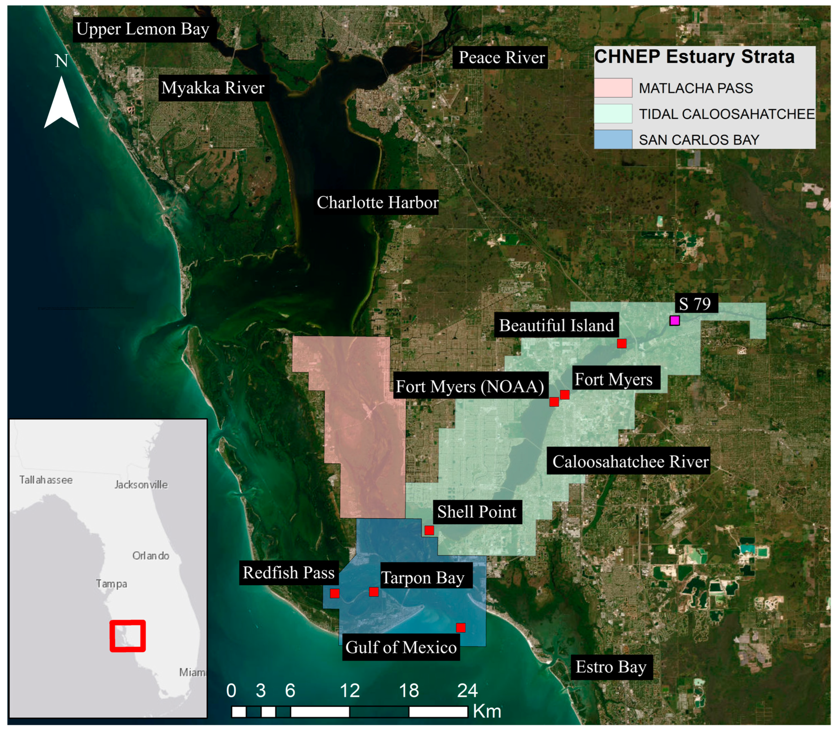
2.1.1. Study Domain and Bathymetry

The numerical model domain covers an area of approximately 800 square kilometers, which spans from Upper Lemon Bay in the north to Estro Bay in the south, with the west boundary situated in the West Florida Shelf (Figure 1a and Figure 2). The model grid consists of a varying horizontal grid resolution ranging from ~300 m offshore to ~10 m in the estuarine regions and inlets (Figure 1b). The water column is discretized with 12 terrain-following vertical layers, which results in a resolution of ~0.1 m in the shallowest parts of the estuary. The bathymetry for the model was constructed using NOAA’s Continuously Updated Digital Elevation Model (CUDEM) with 1/9 arc second resolution and the US Geological Survey’s Lidar Digital Elevation Model for southwest Florida, reconstructed in 2018, with 0.5 m horizontal resolution.

2.1.2. Boundary Conditions and Forcings

The ocean boundaries of the model were forced with free surface elevation, current velocity, water temperature, and salinity acquired from the HYbrid Coordinate Ocean Model with the Naval Research Lab (NRL) Coupled Ocean Data Assimilation Global analysis (HYCOM/NCODA Global), which has an output spatial and temporal resolution of 1/12° and 3 h, respectively. The tidal forcings were acquired from the TPXO global tide model [33]. The Chapman implicit boundary condition was used for the free surface, while the Flather boundary condition was imposed on depth-averaged currents. Radiation boundary conditions were used for water temperature and salinity. A Generic Length Scale approach [34] was used for the vertical turbulence closure scheme in the model.

Bulk atmospheric forcings for the model were obtained from the North American Regional Reanalysis (NARR) [35], which included the 10 m wind speed, atmospheric pressure at mean sea level, 2 m air temperature, relative humidity, and short and longwave radiation. The forcings are available at a 3 h time resolution and a 0.3 degree spatial resolution. Freshwater inflows from the three main rivers in the modeled area (Myakka River, Peace River, and Caloosahatchee River) were acquired from US Geological Survey flow data (https://dashboard.waterdata.usgs.gov/; accessed on 10 January 2022).

2.1.3. Model Calibration

Prior to the production of the final simulations, multiple short-term (~months) calibration runs were performed. Water level, salinity, and water temperature observations gathered by the River, Estuary, and Coastal Observing Network (RECON, https://recon.sccf.org/; accessed on 10 January 2022) were used for calibrating the model. During the calibration process, we observed that the main balance in the estuary is between the bottom friction and the pressure gradient. Hence, the friction coefficients were adjusted to closely match the measurements. The bed stress was calculated using a logarithmic velocity profile with a bed roughness of 0.01 m. Furthermore, an overestimation of the water temperature was observed. After a thorough investigation, we attributed it to an excess of shortwave radiation on the water surface. This bias in the temperature estimation could be due to the effect of cloud coverage not being accounted for in the shortwave radiation data. This issue was resolved by reducing the intensity of the shortwave radiation acquired from NARR by 25%.

After calibrating the model, the numerical model was simulated for a duration of five years, from 1 March 2008, to 1 April 2013.

2.2. Offline Particle Tracking Model

ROMSPath [36] is an offline particle tracking model developed specifically for ROMS model outputs. ROMSPath uses the ROMS native grid to calculate particle trajectories, which reduces the need for interpolation, resulting in increased accuracy over other offline particle tracking models [36]. The model uses the four-dimensional (x, y, z, t) hydrodynamic ROMS outputs to advect passive particles through space and time ($\delta {\mathrm{X}}_{\mathrm{hydro}}$). Furthermore, the model also considers the particle displacement associated with horizontal ($\delta {\mathrm{X}}_{\mathrm{hturb}}$) and vertical diffusion ($\delta {\mathrm{X}}_{\mathrm{vturb}}$). Thus, the particle position vector at a given time can be presented as follows:

$$\mathsf{{\rm X}}(t+\delta t)=\mathrm{}\mathsf{{\rm X}}(t)+\delta {\mathsf{{\rm X}}}_{\mathrm{h}\mathrm{y}\mathrm{d}\mathrm{r}\mathrm{o}}+\delta {\mathsf{{\rm X}}}_{\mathrm{h}\mathrm{t}\mathrm{u}\mathrm{r}\mathrm{b}}+\delta {\mathsf{{\rm X}}}_{\mathrm{v}\mathrm{t}\mathrm{u}\mathrm{r}\mathrm{b}}$$

(1)

where $t$ is time, $\delta t$ is the discrete timestep, and $\mathsf{{\rm X}}(t)$ is the particle position vector in the current time step [36].

ROMSPath uses a fourth-order Runge–Kutta ordinary differential equation solver to calculate the particle advection due to the four-dimensional velocity field ($\delta {\mathsf{{\rm X}}}_{\mathrm{h}\mathrm{y}\mathrm{d}\mathrm{r}\mathrm{o}}$). The vertical random displacements ($\delta {\mathsf{{\rm X}}}_{\mathrm{v}\mathrm{t}\mathrm{u}\mathrm{r}\mathrm{b}}$) of the particles are calculated using a modified random walk method [37]. The vertical turbulent diffusivity derived from the ROMS turbulence closure scheme is used to calculate vertical displacement. The horizontal movement of the particles due to horizontal dispersion ($\delta {\mathsf{{\rm X}}}_{\mathrm{h}\mathrm{t}\mathrm{u}\mathrm{r}\mathrm{b}}$) is also calculated as a random walk using a constant diffusion coefficient of 2.8 m²/s. The order of magnitude of the diffusion coefficient used is in accordance with previous studies with similar flow currents [38].

ROMSpath runs were initiated with particles that were uniformly spread over the estuary (in the horizontal direction and along the water column). A single release case was run for a total duration of 90 days, with multiple such release cases simulated during the simulation period (Section 2.3). The ROMSpath simulation duration was selected as 90 days, as it was observed that this duration was long enough for most particles to move out of the defined region. The location of each particle was recorded at half hour intervals. Particle locations were then used to determine if a particle was either remaining in or had left a given region.

2.3. Calculation of Residence Time and Particle Age

2.3.1. Residence Time

Studies have used multiple parameters (i.e., residence time, flushing time, and turnover time) to describe the time scales required to transport and/or remove material from a given region [38]. In this study, the residence time is defined similarly to that of [17], i.e., the time required for a given water mass to exit a defined region. Past numerical modeling studies (e.g., [23,37]) have released passive concentrations (dye) and tracked the decay of concentrations to calculate the movement of water masses in a region. Another method is using passive particles to track the movement of water masses (e.g., [13]). In this study, we used the latter method as it allowed us to perform multiple different releases of particles and track their movement to calculate residence time.

The Charlotte Harbor estuarine region is divided into 13 strata based on the studies conducted by the Fish and Wildlife Research Institute (FWRI) and the Coastal and Heartland National Estuary Partnership (CHNEP) (Coastal Charlotte Harbor monitoring network-standard operating procedure 2019 updates). Each stratum is considered to have a relatively homogeneous water quality condition. In our study, we used the Tidal Caloosahatchee stratum (Figure 2) as the defined region to calculate residence times in the CRE.

The estuarine residence time, $T_r$ was calculated as follows:

$$T_r=\frac{{\int }_0^{T}N(t)dt}{N(t=0)},$$

(2)

where $N(t=0)$ is the initial number of particles inside the Tidal Caloosahatchee stratum, $N\left(t\right)$ is the number of particles remaining inside the Tidal Caloosahatchee strata at the time $t$. The interval length, $T,$ was chosen as 90 days (ROMSpath simulation duration, Section 2.2) or the time taken for the number of particles to reduce by 10% from the initial value, whichever was the smallest.

A total of 33,440 particles were released in the ROMSPath model uniformly over the entire water body of the Tidal Caloosahatchee strata, and their movements were tracked at ½ h intervals for 90 days. The study consisted of 191 such releases spaced at 10 day intervals. Thus, a total of 6.38 million particles were tracked within the 5 year simulation period.

2.3.2. Particle Age

The particle age was studied in the San Carlos Bay and Matlacha Pass strata, which neighbor the Tidal Caloosahatchee stratum (Figure 2). The intravariation of particle age within these strata was examined by subdividing the stratum into sub-polygons with an approximate size of 200 m × 200 m. The two strata were subdivided into 4727 sub-polygons. The particle age for each sub-polygon was calculated by tracking the number of particles that were residing within each sub-polygon during a release case. The particle age was calculated according to [39] as follows:

$${P_{\mathrm{a}\mathrm{g}\mathrm{e}}}_i=\frac{{\int }_0^T{N}_i\left(t\right)tdt}{{\int }_0^T{N}_i\left(t\right)dt},$$

(3)

where $P_{\mathrm{a}\mathrm{g}{\mathrm{e}}_i}$ is the particle age of the $i^{th}$ sub-polygon and $N_i\left(t\right)$ is the number of particles within the $i^{th}$ sub-polygon at the time $t$.

3. Results

3.1. Model Verification

The model’s performance was evaluated by comparing simulated water levels, salinity, and water temperature time series with measured values along the CRE. Measurements gathered at seven stations (six RECON stations and the NOAA water level gauge at Fort Myers) were used for comparison purposes. Three statistical parameters were used to quantify the model performance: coefficient of determination ($R^2$), root mean square error ($RMSE$), and relative root mean square error ($RRMSE$), computed as follows:

$$R^2=\frac{{\left({\sum }_{i=1}^n({mes}_i-\overline{me{s}_i})({sim}_i-\overline{si{m}_i})\right)}^2}{{{\sum }_{i=1}^n\left({mes}_i-\overline{me{s}_i}\right)}^2{{\sum }_{i=1}^n\left({sim}_i-\overline{{sim}_i}\right)}^2},$$

$$RMSE=\sqrt{\frac{{\sum }_{i=1}^n{\left({mes}_i-{sim}_i\right)}^2}{n}},$$

$$RRMSE=\frac{RMSE}{\left|me{s}_{\mathrm{m}\mathrm{a}\mathrm{x}}-me{s}_{\mathrm{m}\mathrm{i}\mathrm{n}}\right|}\times 100,$$

where $n$ is the number of data points, ${mes}_i$ is the measured value in the field, ${sim}_i$ is the model simulated value, and $me{s}_{\mathrm{m}\mathrm{a}\mathrm{x}}$ and $me{s}_{\mathrm{m}\mathrm{i}\mathrm{n}}$ are measured maximum and minimum values, respectively. Figure 2 depicts the locations of the measurement stations used in the validation.

Table 1. Model error estimates for water level, salinity, and temperature at the measurement locations.

Location	Water Level			Salinity			Temperature
	${\mathit{R}}^2$	$\mathit{R}\mathit{M}\mathit{S}\mathit{E}$ $\left[\mathbf{m}\right]$	$\mathit{R}\mathit{R}\mathit{M}\mathit{S}\mathit{E}$ [%]	${\mathit{R}}^2$	$\mathit{R}\mathit{M}\mathit{S}\mathit{E}$ $\left[\frac{\mathbf{g}}{\mathbf{k}\mathbf{g}}\right]$	$\mathit{R}\mathit{R}\mathit{M}\mathit{S}\mathit{E}$ [%]	${\mathit{R}}^2$	$\mathit{R}\mathit{M}\mathit{S}\mathit{E}$ $\left[\mathbf{C}\right]$	$\mathit{R}\mathit{R}\mathit{M}\mathit{S}\mathit{E}$ [%]
Fort Myers (NOAA)	0.78	0.08	5.50
Beautiful Island	0.85	0.10	9.51
Fort Myers	0.77	0.09	5.96	0.84	4.54	15.38	0.97	1.06	4.73
Shell Point	0.82	0.08	5.57	0.87	3.91	10.20	0.99	0.78	3.09
Tarpon Bay	0.85	0.10	6.76	0.85	2.69	12.07	0.98	0.80	4.41
Gulf of Mexico	0.86	0.10	4.76				0.98	1.01	4.11
Redfish Pass	0.85	0.09	5.66	0.63	1.2	6.91	0.98	0.89	3.66

The gray-shaded areas in Table 1 are due to the unavailability of measurements at the particular station during the hindcast period.

provides a comparison between measured and modeled water levels, salinity, and temperature.

Modeled water levels agree well with the measured water levels (RMSE < 0.11 m) over the simulation period at all locations. Further analysis of the results showed that the model was able to simulate the water level variations that occurred due to high river discharge events and high offshore and onshore wind events. Figure 3 illustrates a time series segment of the model results and the corresponding measured water levels for such a period of high river discharge and wind forcing. The model was able to capture the quick variations in water level during the period of 17 August to 17 September.

Water temperature and salinity observations were measured close to bed level. The model was able to capture the variations in salinity over the simulation period successfully (RMSE < 5). Figure 4 illustrates the salinity variation over the same time interval as the model results in Figure 3. The model was successful in simulating the reduction in salinity as river dominance increased with high river discharge from the 1st of June to the 27th of July. Additionally, the model was able to capture the salinity variations at locations where salt water and fresh water are dynamically mixed (Figure 4).

Similarly, the water temperatures were successfully predicted by the model, which was able to model the temperature fluctuations and trends very well (RMSE < 1.1 °C).

It should be noted that model simulations contain no prior information (e.g., data assimilation using the measured data) on the measured water levels, salinity, or water temperature apart from initialization.

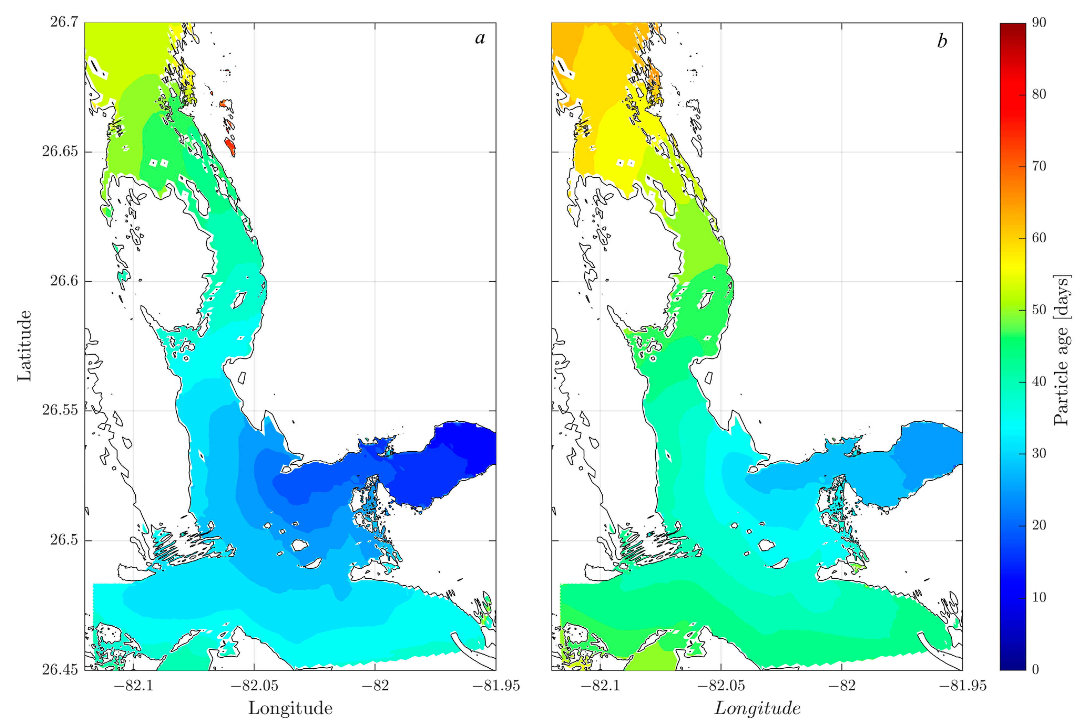
3.2. Particle Movement in the Estuary

Figure 5 provides an example of how the particles move in the estuary with time (release case number 54 on the 15th of June 2009) and the corresponding river discharge, wind magnitude, and direction during that release case. A reduction with time can be observed for the total number of particles as the particles leave the defined region (Tidal Caloosahatchee stratum) for release case 54 (Figure 5d). During the period of 15–30 June, the particles at the downstream end of the estuary are removed from the region (Figure 5b). Most of the particles left the estuary when the river discharge increased between 2 and 10 July (Figure 5c).

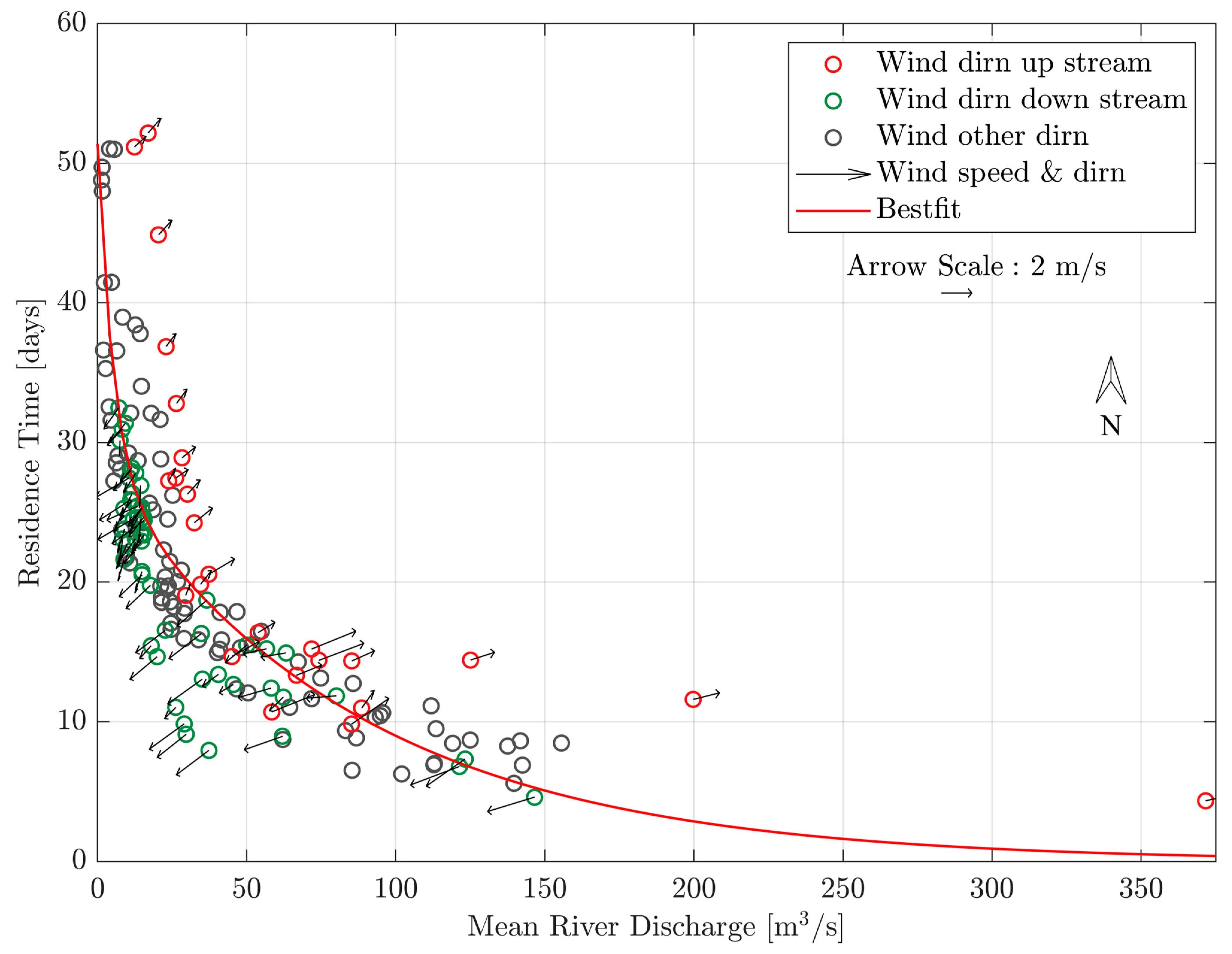
3.3. Effect of River Discharge

The residence times were calculated for all the release cases (191 release cases) over the 5 year study period, using particle track data for each case, similar to that of Figure 5d (release case 54). Figure 6 shows the residence time variation for the Tidal Caloosahatchee stratum over time. A seasonal variation in residence time values can be observed. Furthermore, the seasonal residence time signal shows correspondence to the seasonally varying river discharge. Lower river discharges are correlated with higher residence time events, and vice versa for higher river discharges.

The black dots in Figure 7 represent the residence time values obtained in our study and the corresponding mean river discharge during the releases. Using an optimization workflow based on nonlinear least squares, it was found that a double exponential function was able to best describe ($r^2=0.70$) the relationship between residence time and mean river discharge found in our study (red line in Figure 7). Similar optimization procedures have been conducted in previous studies [40]. The figure also depicts a relationship found in another study (Wan et al. (2013) [23]) at CRE, which is discussed in detail in Section 4.1.

3.4. Effect of Wind Direction and Magnitude on the Residence Time of the Estuary

The residence times are computed using hindcast flow velocities over five years, and thus, wind and other forcings vary between releases. To study the effect of wind on the residence time of the estuary, the mean wind velocity and direction that prevailed during each release duration were calculated. The CRE is aligned along the northeast-southwest axis. Mean wind directions that were directed 45 degrees to either side of the northeast-southwest axis were classified upstream for wind velocities directed between north and east directions and downstream for wind velocities directed between south and west directions.

Figure 8 provides the wind direction and magnitude associated with the release cases where the mean wind velocity was larger than 1 m/s and the wind direction was classified as upstream or downstream. It can be observed that, in general, upstream-directed winds increased the residence time of the estuary while downstream-directed winds decreased it. The effect of wind reduces with increasing mean river discharge. For low river discharge conditions (<50 m³/s), winds can change the residence time by up to 10 days.

4. Discussion

4.1. Use of River Discharge to Explain the Residence Time

Wan et al. (2013) [23] examined the relationship between residence time and river discharge in the CRE by numerically modeling 14 semi-synthetic river discharge scenarios. This study kept the other forcings between the semi-synthetic river discharge scenarios constant. The residence times in that study were computed by releasing an inert tracer concentration and calculating the decay of concentration over time. The study found that a double exponential function best described the relationship between residence time and river discharge (blue line in Figure 7). In their study, the river discharge fully explained the residence time variation (the $r^2\&gt;0.99$ for the relationship between river discharge and residence time obtained in that study) as it was the only variable. While other forces (e.g., wind and tidal conditions) are variable between releases in our study, the residence time variations in the estuary can still be explained to a good extent by the mean river discharge. The average difference among the residence time predictions between our study and [23] is 2.44 days (red and blue lines in Figure 7). However, it can be observed in Figure 8 that the wind velocity and direction act as secondary forces, changing the residence time. The wind forcing has the highest effect on the residence time at low discharge conditions, which is observed in the dry season (the average Caloosahatchee River discharge during the dry season $<38.5 {\mathrm{m}}^3/\mathrm{s}$). Figure 9 depicts the wind velocities and directions measured by the NOAA gauge at Fort Myers, FL, during the dry season (June to October). It can be observed that the winds are predominantly directed in the downstream direction of the estuary during the dry season. The downstream-directed wind helps the particle leave the estuary, reducing the residence time compared to particle dispersal only due to river discharge. The mean difference between the red and blue lines in Figure 7 for river discharge $<38.5 {\mathrm{m}}^3/\mathrm{s}$ increases to 6.98 days from the average of 2.44 days.

At higher discharges, the effect of wind forcing becomes smaller, and the residence time is predominantly governed by the river discharge. The mean difference between the red and blue lines in Figure 7 for river discharge $\&gt;38.5{\mathrm{m}}^3/\mathrm{s}$ is 1.86 days. A similar seasonal wind effect on particle movement in the CRE and Charlotte Harbor Estuary was observed in the study by Dye et al. (2020) [30].

4.2. Effect of River Mass Transport and Density-Induced Circulation on Residence Time

The effect of river discharge on residence time is twofold. The downstream mass flux caused by the river discharge carries particles from the defined region. Furthermore, the freshwater discharge of the river induces density gradient currents in the estuary, which can also result in a subtidal flow [41]. While these subtidal flows are much weaker than the flow due to the mass flux of the river, they can have disproportionately greater importance in the movement of waterborne material [42]. To study the importance of density gradient-induced circulation on residence times, the hydrodynamic model was rerun without density-induced circulation by using zero salinity all over the model domain. The resulting velocity fields were then used to calculate the particle transport and the corresponding residence times.

Figure 10 provides the residence time variation with river discharge with and without density-induced circulations. It should be noted that not all cases were simulated with the zero salinity condition due to computational expense. All releases in non-density-induced circulations resulted in a higher residence time (an average increase of 10 days) compared to the original (Figure 10b). With increasing river discharge, the difference starts to reduce as the density-induced circulation becomes weaker and the particle movements are influenced mostly due to mass flow from the river. Similar results were also observed by [18] in the Danshuei River estuarine system in Taiwan. The authors observed that disregarding density gradient-induced circulations resulted in higher residence times, and the effect of the water density gradient-induced circulation was reduced with increasing river discharge.

4.3. Particle Age at the Neighboring Strata

The Caloosahatchee River conveys pollutants/nutrients it receives from Lake Okeechobee and the watershed to the coastal and estuarine systems [43]. The particle age of the neighboring two strata to CRE (i.e., San Carlos Bay and Matlacha Pass) can provide information on where the pollutants/nutrients remain the longest. The particle age was calculated for these two strata according to Equation (3) for all release cases. The average particle age was then calculated for the dry and wet periods in the system (The wet season was taken as November to April, and the dry season was taken as June to October [22]. Figure 11 provides the particle age variation in San Carlos Bay and the Matlacha Pass for the wet and dry seasons. A clear variation in the particle age between the two seasons can be observed. The wet season in general shows a lower particle age compared to the dry season. The dominance of the riverine processes during the wet season is especially apparent at the mouth of the CRE, where the particle age is lower as the river can quickly push the particles further away. In both wet and dry seasons, the Matlacha Pass shows a higher particle age compared to San Carlos Bay. These results suggest that Matlacha Pass could have a higher probability than San Carlos Bay of having water quality issues due to pollutant discharge from the CRE.

4.4. Influence of Particle Buoyancy on Residence Time

The particles that were used in our study were neutrally buoyant and resembled “passive traces” which are free to travel through the whole water column due to the advection and diffusion processes. However, certain pollutants and nutrients that are transported in estuarine environments can also be either positively or negatively buoyant. Locations at which the particles reside in the water column will affect their movement and, hence, the residence time of the estuary. Particle tracking models compute vertical movements using ad hoc methods [44]. In our study, we used a similar technique to replicate the effects of positive and negative buoyancy instead of solving all the complex physics. The residence time of positively or negatively buoyant particles was studied by constraining the movement of the particles to only a 25 cm layer on the surface of the water column (positively buoyant particles) and a 25 cm layer on the bottom of the water column (negatively buoyant particles). This approach is deemed a reasonable approximation for the horizontal movement of these particles, which are mainly affected by the horizontal currents. Similar methods have been used in previous studies [45]. Figure 12 provides the residence times obtained for these two cases compared with the neutrally buoyant particle results (original results presented in Section 3.3). The positively buoyant particle residence time is much smaller compared to the neutrally buoyant particles. The average residence time was 22.2 days for neutrally buoyant particles, compared to just 9.6 days for positively buoyant particles. Furthermore, the positively buoyant particles only showed a reduction in residence time with increasing river discharge at low river dischargers (mean river dischargers < 20 m³/s). The residence time values became invariant on river discharge for discharges larger than 20 m³/s.

The near-bottom subtidal velocities are much smaller than in the rest of the water column and are generally oriented in the upstream direction in the river estuary. The bottom velocity at the estuary mouth was on average 4–6 times smaller compared to the depth-averaged velocity. As a result, negatively buoyant particles are unable to leave the defined region during low discharge events, leading to residence times that are longer than 80 days for release cases with a mean river discharge smaller than 60 m³/s. When the river discharge is sufficiently large, the bottom velocities can also be directed downstream and carry the particles off the defined region, reducing the residence time. For negatively buoyant particles, a threshold on the river discharge (~60 m³/s) can be observed for the particles to leave the estuarine area. Further, a large variation in the residence time is observed for a given mean river discharge for negatively buoyant particles.

Figure 13 provides the number of particles remaining within the region in time for the release cases with negatively buoyant particles marked in Figure 12 ($R{C}_{56},$  $R{C}_{18}$, and $R{C}_{25}$). While the mean river discharge is approximately the same for these three release cases, the discharge time series varies between them (Figure 13b). The river flows that occurred during $R{C}_{25}$ and $R{C}_{18}$ show large pulses of discharge, and much of the particle movement off the defined region only occurred at these large river pulses ($R{C}_{25}$ and $R{C}_{18}$, Figure 13a). On the contrary, only a few particles move out of the defined region during $R{C}_{56}$, as the river discharge does not have such large pulses that are able to push the particles out of the defined region. The residence time thus varies by a large amount (a 54 day difference between $R{C}_{25}$ and $R{C}_{56}$) even though they have the same mean river discharge.

4.5. Implications of Residence Time on Water Quality

Water quality issues in an estuary (e.g., eutrophication) depend on nutrient loading, biogeochemical processes, and residence time [13]. The concentration of many nutrients (e.g., Ammonia-n (NH₄) Nitrates, Total Nitrogen-n) increased with increasing river discharge in the CRE [26,46]. However, the increase in nutrient loads in the wet season did not result in a similar increase in chlorophyll concentrations, a proxy for phytoplankton blooms [46]. Rumbold (2023) [46] hypothesized this was due to the “flushing” of the estuary, which removes the nutrients from the area. In our study, we observed an exponential reduction in residence time with increasing river discharge, which justifies the results and the hypothesis made in [46].

In our study, we also observed a seasonal signal in residence time (Figure 6), where low residence time periods (which correspond to high river discharge) are followed by high residence time periods. Large algal blooms have occurred in the CRE following tropical storms and hurricanes [47,48]. These algal blooms could be partly fueled by the comparatively high residence times (>20 days) in the estuaries, which occur after high discharge events such as storms.

The nutrient loading to the CRE by the Caloosahatchee River is dependent on the type of discharge (i.e., release from Lake Okeechobee and/or watershed runoff) [26]. Furthermore, the water management operations on Lake Okeechobee also affect the nutrient concentrations received by the CRE [49]. Future studies, including the nutrient loading and coupling of the hydrodynamic model with biogeochemistry modules, will be required to generate a holistic picture of water quality in the CRE region.

4.6. Applicability of the Findings to Other Estuaries and Further Considerations

While most of the results obtained on the influence of processes on residence time at CRE can be transferred to other estuaries, some aspects need to be considered. The residence time of an estuary is dependent on its geometry and morphological characteristics. The CRE is a long estuary with a single opening to the ocean. An estuary with more complex geometry may show different results, especially due to wind action [50]. Furthermore, the CRE is micro-tidal, and therefore, estuaries with larger tidal ranges may show variations in the results (e.g., [51]). Another unique aspect of CRE is that its freshwater discharge is heavily regulated, which will change river discharge patterns in a natural estuarine river.

Bathymetry plays an important role in the circulation of the estuary. In our model, we keep the bathymetry constant over time. While there have been no major changes to the bathymetry during the study period, large storms like Hurricane Ian in 2022 can change the bathymetry rapidly. The model bathymetry can be updated as needed using methods such as satellite-derived bathymetry [52] to improve the circulation in the system and thus the residence time and particle age calculations.

5. Conclusions

The primary objective of this study was to understand how residence time was influenced by different forcings and processes at the CRE, a subtropical estuary strongly influenced by managed river discharges. The study was conducted by performing a multiyear hindcast. The residence time of the estuary was mainly controlled by the river discharge, with a double exponential function best describing the decreasing trend of the residence time with increasing mean river discharge. The residence-time time series over a five year period showed a strong seasonal signal. Wind velocity and magnitude also affected the residence time. Wind velocities directed in the downstream direction tended to reduce the residence time, while upstream-directed wind velocities increased the residence time. The effect of wind velocity on residence time decreased with increasing discharge. Water density gradient-induced circulations were observed to reduce residence time on average by 10 days. Finally, the buoyancy of the particles also influenced the residence time: positively buoyant particles, which remained at the surface of the estuary, had a smaller residence time compared to negatively buoyant particles, which remained near the bottom of the estuary.

References

1. Constanza, R.; Kemp, W.M.; Boynton, W.R. Predictability, scale, and biodiversity in coastal and estuarine ecosystems: Implications for management. Ambio 1993, 22, 88–96. [Google Scholar] [CrossRef]
2. Lellis-Dibble, K.A.; McGlynn, K.E.; Bigford, T.E. Estuarine Fish and Shellfish Species in US Commercial and Recreational Fisheries: Economic Value as an Incentive to Protect and Restore Estuarine Habitat. 2008. Available online: https://repository.library.noaa.gov/view/noaa/3612/noaa_3612_DS1.pdf (accessed on 1 January 2023).
3. Jarvie, H.P.; Jickells, T.D.; Skeffington, R.A.; Withers, P.J.A. Climate change and coupling of macronutrient cycles along the atmospheric, terrestrial, freshwater and estuarine continuum. Sci. Total Environ. 2012, 434, 252–258. [Google Scholar] [CrossRef] [PubMed]
4. Statham, P.J. Nutrients in estuaries—An overview and the potential impacts of climate change. Sci. Total Environ. 2012, 434, 213–227. [Google Scholar] [CrossRef]
5. Schettini, C.A.F.; Valle-Levinson, A.; Truccolo, E.C. Circulation and transport in short, low-inflow estuaries under anthropogenic stresses. Reg. Stud. Mar. Sci. 2017, 10, 52–64. [Google Scholar] [CrossRef]
6. Prandle, D. Estuaries: Dynamics, Mixing, Sedimentation and Morphology; Cambridge University Press: Cambridge, UK, 2009. [Google Scholar]
7. Valle-Levinson, A. Contemporary Issues in Estuarine Physics; Cambridge University Press: Cambridge, UK, 2010. [Google Scholar]
8. Ganju, N.K.; Brush, M.J.; Rashleigh, B.; Aretxabaleta, A.L.; Del Barrio, P.; Grear, J.S.; Harris, L.A.; Lake, S.J.; McCardell, G.; O’Donnell, J.; et al. Progress and Challenges in Coupled Hydrodynamic-Ecological Estuarine Modeling. Estuaries Coasts 2016, 39, 311–332. [Google Scholar] [CrossRef] [Green Version]
9. Jay, D.A.; Uncles, R.J.; Largier, J.; Geyer, W.R.; Vallino, J.; Boynton, W.R. A review of recent developments in estuarine scalar flux estimation. Estuaries 1997, 20, 262–280. [Google Scholar] [CrossRef]
10. Rasmussen, B.; Josefson, A.B. Consistent estimates for the residence time of micro-tidal estuaries. Estuar. Coast. Shelf Sci. 2002, 54, 65–73. [Google Scholar] [CrossRef]
11. González, F.U.T.; Herrera-Silveira, J.A.; Aguirre-Macedo, M.L. Water quality variability and eutrophic trends in karstic tropical coastal lagoons of the Yucatán Peninsula. Estuar. Coast. Shelf Sci. 2008, 76, 418–430. [Google Scholar] [CrossRef]
12. Paerl, H.W. Nuisance phytoplankton blooms in coastal, estuarine, and inland waters 1. Limnol. Oceanogr. 1988, 33, 823–843. [Google Scholar] [CrossRef]
13. Defne, Z.; Ganju, N.K. Quantifying the Residence Time and Flushing Characteristics of a Shallow, Back-Barrier Estuary: Application of Hydrodynamic and Particle Tracking Models. Estuaries Coasts 2015, 38, 1719–1734. [Google Scholar] [CrossRef]
14. Jassby, A.; Van Nieuwenhuyse, E.E. Low dissolved oxygen in an estuarine channel (San Joaquin River, California): Mechanisms and models based on long-term time series. San Fr. Estuary Watershed Sci. 2005. [Google Scholar] [CrossRef] [Green Version]
15. Salas-Monreal, D.; Valle-Levinson, A. Sea-level slopes and volume fluxes produced by atmospheric forcing in estuaries: Chesapeake Bay case study. J. Coast. Res. 2008, 24 (Suppl. B), 208–217. [Google Scholar] [CrossRef] [Green Version]
16. Monsen, N.E.; Cloern, J.E.; Lucas, L.V.; Monismith, S.G. A comment on the use of flushing time, residence time, and age as transport time scales. Limnol. Oceanogr. 2002, 47, 1545–1553. [Google Scholar] [CrossRef] [Green Version]
17. Zimmerman, J.T.F. Mixing and flushing of tidal embayments in the western Dutch Wadden Sea part I: Distribution of salinity and calculation of mixing time scales. Neth. J. Sea Res. 1976, 10, 149–191. [Google Scholar] [CrossRef]
18. Liu, W.; Chen, W.; Kuo, J.; Wu, C. Numerical determination of residence time and age in a partially mixed estuary using three-dimensional hydrodynamic model. Cont. Shelf Res. 2008, 28, 1068–1088. [Google Scholar] [CrossRef]
19. Zheng, L.; Weisberg, R.H. Tide, bouyancy, and wind-driven circulation of the Charlotte Harbor estuary: A model study. J. Geophys. Res. Ocean. 2004, 109, 1–16. [Google Scholar] [CrossRef] [Green Version]
20. Chamberlain, R.H.; Doering, P.H. Freshwater Inflow to the Caloosahatchee Estuary and the Resource-Based Method for Evaluation; Ecosystem Restoration Department, South Florida Water Management District: Punta Gorda, FL, USA, 1998. [Google Scholar]
21. Shi, L.; Ortals, C.; Valle-Levinson, A.; Olabarrieta, M. Influence of river discharge on tidal and subtidal flows in a microtidal estuary: Implication on velocity asymmetries. Adv. Water Resour. 2023, 177, 104446. [Google Scholar] [CrossRef]
22. Qiu, C.; Wan, Y. Time series modeling and prediction of salinity in the Caloosahatchee River Estuary. Water Resour. Res. 2013, 49, 5804–5816. [Google Scholar] [CrossRef]
23. Wan, Y.; Qiu, C.; Doering, P.; Ashton, M.; Sun, D.; Coley, T. Modeling residence time with a three-dimensional hydrodynamic model: Linkage with chlorophyll a in a subtropical estuary. Ecol. Modell. 2013, 268, 93–102. [Google Scholar] [CrossRef]
24. Cifuentes, L.A.; Schemel, L.E.; Sharp, J.H. Qualitative and numerical analyses of the effects of river inflow variations on mixing diagrams in estuaries. Estuar. Coast. Shelf Sci. 1990, 30, 411–427. [Google Scholar] [CrossRef]
25. Doering, P.H.; Chamberlain, R.H. Water quality and source of freshwater discharge to the caloosahatchee estuary, florida. JAWRA J. Am. Water Resour. Assoc. 1999, 35, 793–806. [Google Scholar] [CrossRef]
26. Rumbold, D.G.; Doering, P.H. Water quality and source of freshwater discharge to the Caloosahatchee Estuary, Florida. Fla. Sci. 2020, 83, 1–20. Available online: https://www.jstor.org/stable/26975620 (accessed on 1 January 2023).
27. Urakawa, H.; Steele, J.H.; Hancock, T.L.; Dahedl, E.K.; Schroeder, E.R.; Sereda, J.V.; Kratz, M.A.; García, P.E.; Armstrong, R.A. Interaction among spring phytoplankton succession, water discharge patterns, and hydrogen peroxide dynamics in the Caloosahatchee River in southwest Florida. Harmful Algae 2023, 126, 102434. [Google Scholar] [CrossRef] [PubMed]
28. Xia, M.; Craig, P.M.; Schaeffer, B.; Stoddard, A.; Liu, Z.; Peng, M.; Zhang, H.; Wallen, C.M.; Bailey, N.; Mandrup-Poulsen, J. Influence of Physical Forcing on Bottom-Water Dissolved Oxygen within Caloosahatchee River Estuary, Florida. J. Environ. Eng. 2010, 136, 1032–1044. [Google Scholar] [CrossRef]
29. Chen, Z.; Doering, P.H.; Ashton, M.; Orlando, B.A. Mixing Behavior of Colored Dissolved Organic Matter and Its Potential Ecological Implication in the Caloosahatchee River Estuary, Florida. Estuaries Coasts 2015, 38, 1706–1718. [Google Scholar] [CrossRef]
30. Dye, B.; Jose, F.; Allahdadi, M.N. Circulation Dynamics and Seasonal Variability for the Charlotte Harbor Estuary, Southwest Florida Coast. J. Coast. Res. 2020, 36, 276–288. [Google Scholar] [CrossRef]
31. Shchepetkin, A.F.; McWilliams, J.C. The regional oceanic modeling system (ROMS): A split-explicit, free-surface, topography-following-coordinate oceanic model. Ocean Model. 2005, 9, 347–404. [Google Scholar] [CrossRef]
32. Haidvogel, D.B.; Arango, H.; Budgell, W.P.; Cornuelle, B.D.; Curchitser, E.; Di Lorenzo, E.; Fennel, K.; Geyer, W.R.; Hermann, A.J.; Lanerolle, L.; et al. Ocean forecasting in terrain-following coordinates: Formulation and skill assessment of the Regional Ocean Modeling System. J. Comput. Phys. 2008, 227, 3595–3624. [Google Scholar] [CrossRef]
33. Egbert, G.D.; Erofeeva, S.Y. Efficient Inverse Modeling of Barotropic Ocean Tides. J. Atmos. Ocean. Technol. 2002, 19, 183–204. [Google Scholar]
34. Warner, J.C.; Sherwood, C.R.; Arango, H.G.; Signell, R.P. Performance of four turbulence closure models implemented using a generic length scale method. Ocean Model. 2005, 8, 81–113. [Google Scholar] [CrossRef]
35. Mesinger, F.; DiMego, G.; Kalnay, E.; Mitchell, K.; Shafran, P.C.; Ebisuzaki, W.; Jović, D.; Woollen, J.; Rogers, E.; Berbery, E.H.; et al. North American Regional Reanalysis. Bull. Am. Meteorol. Soc. 2006, 87, 343–360. [Google Scholar] [CrossRef] [Green Version]
36. Hunter, E.J.; Fuchs, H.L.; Wilkin, J.L.; Gerbi, G.P.; Chant, R.J.; Garwood, J.C. ROMSPath v1.0: Offline particle tracking for the Regional Ocean Modeling System (ROMS). Geosci. Model Dev. 2022, 15, 4297–4311. [Google Scholar] [CrossRef]
37. Visser, A.W. Using random walk models to simulate the vertical distribution of particles in a turbulent water column. Mar. Ecol. Prog. Ser. 1997, 158, 275–281. [Google Scholar] [CrossRef] [Green Version]
38. Cucco, A.; Umgiesser, G. Modeling the Venice Lagoon residence time. Ecol. Modell. 2006, 193, 34–51. [Google Scholar] [CrossRef]
39. Sandberg, M. What is ventilation efficiency? Build. Environ. 1981, 16, 123–135. [Google Scholar] [CrossRef]
40. Hewageegana, V.H.; Bilskie, M.V.; Woodson, C.B.; Bledsoe, B.P. The effects of coastal marsh geometry and surge scales on water level attenuation. Ecol. Eng. 2022, 185, 106813. [Google Scholar] [CrossRef]
41. Smith, R. Longitudinal dispersion of a buoyant contaminant in a shallow channel. J. Fluid Mech. 1976, 78, 677–688. [Google Scholar] [CrossRef]
42. Geyer, W.R.; MacCready, P. The estuarine circulation. Annu. Rev. Fluid Mech. 2014, 46, 175–197. [Google Scholar] [CrossRef]
43. Medina, M.; Kaplan, D.; Milbrandt, E.C.; Tomasko, D.; Huffaker, R.; Angelini, C. Nitrogen-enriched discharges from a highly managed watershed intensify red tide (Karenia brevis) blooms in southwest Florida. Sci. Total Environ. 2022, 827, 154149. [Google Scholar] [CrossRef]
44. Lange, M.; Van Sebille, E. Parcels v0.9: Prototyping a Lagrangian ocean analysis framework for the petascale age. Geosci. Model Dev. 2017, 10, 4175–4186. [Google Scholar] [CrossRef] [Green Version]
45. Liang, J.H.; Liu, J.; Benfield, M.; Justic, D.; Holstein, D.; Liu, B.; Hetland, R.; Kobashi, D.; Dong, C.; Dong, W. Including the effects of subsurface currents on buoyant particles in Lagrangian particle tracking models: Model development and its application to the study of riverborne plastics over the Louisiana/Texas shelf. Ocean Model. 2021, 167, 101879. [Google Scholar] [CrossRef]
46. Rumbold, D.G. Use of a Bayesian network as a decision support tool for watershed management: A case study in a highly managed river-dominated estuary. Environ. Monit. Assess. 2023, 195, 741. [Google Scholar] [CrossRef] [PubMed]
47. Glibert, P.M. Harmful algae at the complex nexus of eutrophication and climate change. Harmful Algae 2020, 91, 101583. [Google Scholar] [CrossRef] [PubMed]
48. Brewton, R.A.; Kreiger, L.B.; Tyre, K.N.; Baladi, D.; Wilking, L.E.; Herren, L.W.; Lapointe, B.E. Septic system–groundwater–surface water couplings in waterfront communities contribute to harmful algal blooms in Southwest Florida. Sci. Total Environ. 2022, 837, 155319. [Google Scholar] [CrossRef]
49. Tarabih, O.M.; Arias, M.E. Hydrological and Water Quality Trends through the Lens of Historical Operation Schedules in Lake Okeechobee. J. Water Resour. Plan. Manag. 2021, 147, 04021034. [Google Scholar] [CrossRef]
50. Montaño-Ley, Y.; Soto-Jiménez, M.F. A numerical investigation of the influence time distribution in a shallow coastal lagoon environment of the Gulf of California. Environ. Fluid Mech. 2019, 19, 137–155. [Google Scholar] [CrossRef]
51. Yuan, D.; Lin, B.; Falconer, R.A. A modelling study of residence time in a macro-tidal estuary. Estuar. Coast. Shelf Sci. 2007, 71, 401–411. [Google Scholar] [CrossRef]
52. Mudiyanselage, S.S.J.D.; Wilkinson, B.; Lecours, V.; Wilkinson, B.; Lecours, V. Satellite-derived bathymetry using machine learning and optimal Sentinel-2 imagery in South-West Florida coastal waters ABSTRACT. GISci. Remote Sens. 2022, 59, 1143–1158. [Google Scholar] [CrossRef]
Figure 1. (a) Numerical model domain and bathymetry. (b) Grid resolution in the wet region of the model is computed as the square root of the area of grid cells.
Jmse 11 01333 g001
Figure 2. Study location. The polygons represent the Coastal and Heartland National Estuary Partnership (CHNEP) demarcated strata near the CRE. The red squares represent the monitoring stations (maintained by RECON and NOAA) used for the validation of water level, salinity, and temperature. The purple square represents the Franklin Lock and Dam (S-79) location.
Jmse 11 01333 g002
Figure 3. (ae) Modeled and measured water level signals at observation locations are represented in red and black lines, respectively. (f) Caloosahatchee River discharge at S-79. (g) Average wind speed and direction in the Tidal Caloosahatchee strata. The blue arrows depict the direction of the winds, corresponding to the north arrow of the figure. The days are in the year 2008.
Jmse 11 01333 g003
Figure 4. (ac) Modeled and measured salinity signals at observation locations, represented in red and black lines, respectively. (d) Caloosahatchee River discharge at S79. The days are in the year 2008.
Jmse 11 01333 g004
Figure 5. Particle movement in the CRE. (ac) Number of particles per 10 4   m 2 at 0, 10, and 20 days after the release of particles, respectively, for release case 54 (released on 15th June 2009 (T)). (d) The total number of particles remaining in the Tidal Caloosahatchee stratum for release case 54. (e) Caloosahatchee river discharge at S-79. (f) Average wind speed and direction in the Tidal Caloosahatchee stratum. The days are in the year 2009.
Jmse 11 01333 g005
Figure 6. (a) Residence time variation over time. The black dots show the residence time values for each release case, and the red line depicts the fitted spline to the calculated residence time values. (b) Mean river discharge variation over time. The black dots show the mean river discharge for each release case, and the red line depicts the fitted spline to the mean river discharge values.
Jmse 11 01333 g006
Figure 7. Residence time variation with mean river discharge for the release cases (black dots). The red line indicates the best-fit double-exponential curve for the data. The equation for the best-fit curve is provided in the figure, where y is the residence time and x is the mean river discharge. The blue line indicates the Wan et al. (2013) [23] study results.
Jmse 11 01333 g007
Figure 8. Effect of wind magnitude and direction on residence time. The arrows show the magnitude and direction of the average wind speed during the release case. The arrow direction is drawn in relation to the north arrow shown in the figure. The red, green, and black dots represent the wind direction classification for the release case: upstream, downstream of CRE, and other directions, respectively for the release case. The red line represents the best-fit curve for the data (Figure 7).
Jmse 11 01333 g008
Figure 9. The wind rose for CRE during the dry season (June to October) for the study period. The direction shown is the “wind is blowing to” direction.
Jmse 11 01333 g009
Figure 10. Effect of density-induced circulation on the residence time of the estuary. (a) The black line represents the relationship obtained for residence time vs. river discharge with density-induced circulation (red line in Figure 7). The blue dots represent the residence time and mean river discharge for the release cases without density-induced circulation. The blue line indicates the best-fit double-exponential curve for the blue dots data. (b) The black dots depict the difference in residence time between with and without density-induced circulation for each case ( R e s i d e n c e   T i m e w /   d e n s i t y   i n d u c e d   c i r c R e s i d e n c e   T i m e w / o .   d e n s i t y   i n d u c e d   c i r c ) . The black line represents the fit of the double exponential curve to the data.
Jmse 11 01333 g010
Figure 11. Average particle age (days) in the San Carlos Bay and Matlacha Pass during the (a) wet and (b) dry seasons.
Jmse 11 01333 g011
Figure 12. Residence time variation with the buoyancy of the particles. The red dots represent the residence time for particles constrained to the surface (positively buoyant particles). The blue dots depict the residence time for particles constrained to the bottom (negatively buoyant particles). The red (double exponential) and blue (two-term power series model) lines represent the best-fit curves for the red and blue dots, respectively. The black line represents the residence time variation for the neutrally buoyant particles.
Jmse 11 01333 g012
Figure 13. Particle movement out of tidal Caloosahatchee strata for particles only at the bottom. (a) The number of particles remaining in tidal Caloosahatchee strata after release for release cases 56, 18, and 25 is represented by orange, green, and purple lines, respectively. (b) The time series of river discharge prevailing during each release case (i.e., release cases 56, 18, and 25).
Jmse 11 01333 g013