1. Introduction
1.1. Current Status of Marine Oil Spill Research
Oil has always been a necessity that is inseparable from modern industrial production and social life. With the increase in research and exploration of the ocean, the exploitation of offshore oil fields has gradually become the main way to obtain oil energy. At the same time, the increase in the number of offshore oil fields and ocean-going tanker voyages has greatly increased the risk of oil spills at sea [
1]. The effect of oil spills on the marine ecosystem is extremely severe. For example, the blowout explosion of the Deepwater Horizon rig in the Gulf of Mexico in 2010 spilled about 3.2 million barrels of oil and covered at least 2500 km
2 of seawater [
2,
3]. In order to avoid the continuous damage to the marine environment caused by similar events, we need to accurately delineate the sea surface oil spill area and provide data support for the emergency treatment of sea surface oil spill events as much as possible.
Aerospace remote sensing can survey Earth from different heights, ranges, velocities and spectral bands to obtain a large amount of information. Therefore, remote sensing technology has gained wide application in many aspects of the national economy and military, such as weather prediction, resource inspection and environmental monitoring. Due to the advantages of hyperspectral sensors with many spectral bands and large spatial capacity, hyperspectral images have great potential in oil spill research compared with other technical means [
4,
5]. Although the quality of hyperspectral imaging is affected by environmental factors such as weather and light, its unique spectral features can compensate for the deficiencies caused by environmental factors in the an oil spill area to provide high-value information that can distinguish between oil spill and water surface features, thus identifying information related to the oil spill area and making oil film thickness estimation possible [
6,
7,
8].
With the full utilization of different depth features, deep learning plays an important role in image segmentation, target detection, etc. [
9,
10]. Deep learning is widely used in the research of hyperspectral images, to study their rich spectral and spatial information. At present, deep learning mainly combines the spectral features, spatial features and spatial spectral features of hyperspectral images in image research. For example, Chen [
11] and Hu [
12] proposed CNN models using the spectral features of original images for the target detection of different task types. However, hyperspectral images are susceptible to adjacent pixels and mixed pixels, and using only spectral information is likely to cause classification errors; so, scholars have begun to attempt classification using spatial information [
13]. Guidici [
14] extracted some spatial features from hyperspectral data using CNN models for studying land cover classification, and concluded via experiments that 1D CNNs are in some cases more advantageous than 3D CNNs as they can be less computationally intensive. The experimental results have room for improvement as only the information between a certain pixel point on the image is considered and the unique spectral information of hyperspectral images was not utilized. Li [
15] used 3D CNNs to classify images by combining spectral and spatial information for deep feature extraction, and the effect was significantly improved. Although combining spectral and spatial information can make full use of the information of hyperspectral images and improve the classification accuracy of hyperspectral images to some extent, this significantly increases the computation time compared with the first two approaches [
10,
16].
1.2. Related Work
Relevant research will be reviewed in this section, including on the Gulf of Mexico oil spill, segmentation networks, residual networks and attention mechanisms.
1.2.1. The Gulf of Mexico Oil Spill
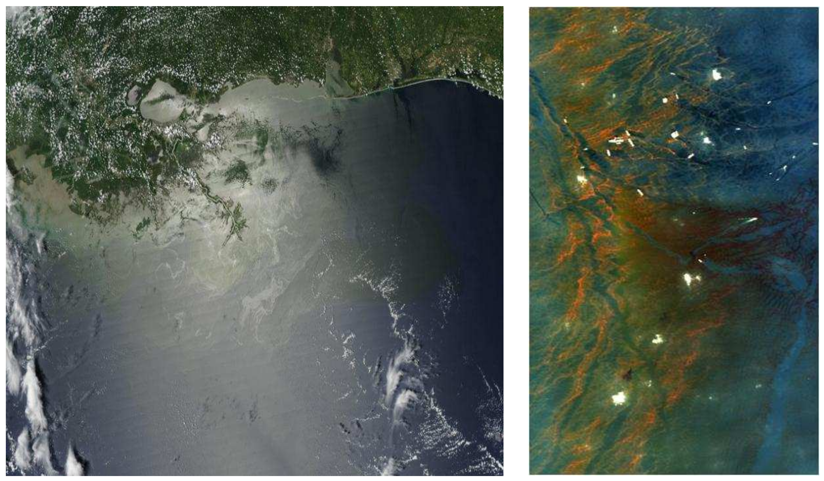
The 2010 Gulf of Mexico oil spill was one of the worst crude oil spills in history [
2], as
Figure 1 shows. Crude oil erupted from the Deepwater Horizon deep-sea rig, and the spill lasted for three months, causing continuous damage to the marine environment. The study of this is a good source of publicly available datasets via hyperspectral image acquisition in NASA laboratories. NASA’s Airborne Visible/Infrared Imaging Spectrometer (AVIRI-S) measured a total of more than 100,000 km
2 of ocean during the spill to help scientists and the relevant authorities to better understand the spill and how to address its effects [
17,
18]. The data in this study are based on AVIRIS, recording 224 bands in the wavelength range of 400–2500
.
1.2.2. Segmentation Networks
When it comes to deep learning methods, fully supervised learning methods are more effective than semi-supervised learning methods [
19]. Upon its introduction, Deeplabv3+ [
20] was considered to be one of the most effective semantic segmentation models, achieving satisfactory segmentation results when applied to many public datasets, such as the PASCAL VOC2012 dataset [
21] and the City Scapes dataset [
22]. The network of Deeplabv3+ is divided into two main parts: the encoder and the decoder. The encoder fully exploits the multi-scale contextual features of the images using the atrous spatial pyramid pooling (ASPP) module. The decoder uses shallow feature maps to optimize the information that cannot be recovered via upsampling, and finally obtains the semantic segmentation results.
1.2.3. Residual Network
As the deep learning model deepens, it leads to a larger number of non-linear layers, causing the more non-linear fitting ability of the model and reducing the generalization ability. Some layers in the residual network skip the connection of neurons in the next layer and are connected in alternate layers, which can weaken the connection between each layer and enhance the linear fitting ability [
23]. The residual network is proposed to simplify the training of deeper neural networks. The network does not suffer from gradient disappearance nor gradient explosion during the node updating of node parameters, and solves the network degradation problem. Although the residual network extracts rich features, it does not evaluate these features and does not make full use of the features on different scales to improve the efficiency of the model.
1.2.4. Attention Mechanisms
Attention mechanisms were first used in natural language processing, where the main goal was to focus on important features and suppress unnecessary ones [
24,
25,
26]. As research progresses, attention mechanisms are now increasingly used in a wide range of fields, such as image classification, target detection, medical image analysis, etc. Attention mechanisms are mainly classified into spatial attention mechanisms, channel attention mechanisms and hybrid attention mechanisms.
Channel attention refers to changing the weights on each channel to enhance the learning of a specific channel, thus improving the performance of the model [
27]. The input feature map is passed through two parallel maximum pooling layers and average pooling layers to compress the spatial dimension of the feature map, and the number of channels is compressed and re-expanded using the Share MLP module to recover it to the number of channels of the original map. The maximum pooling layer and the average pooling layer are operational layers used to reduce the spatial dimension of the feature map. The maximum pooling layer retains the most significant features, while the average pooling layer smoothes the features. The two results after activation via the ReLU function are added row by row, and finally activated via a sigmoid function to obtain the output of the channel attention mechanism, which is then multiplied using the original map to recover it to the original feature map size.
Unlike the channel attention mechanism, the spatial attention mechanism focuses on the “where”, which is complementary to the channel attention mechanism [
28]. The feature map of the spatial attention mechanism is generated by concatenating the results of the maximum pooling layer and the average pooling layer, and then concatenating the results through a standard convolutional layer.
The hybrid attention mechanism is a simple and effective attention module for feedforward convolutional neural networks [
29]. With a given intermediate feature map, the module infers the attention map along two different dimensions, channel and space, and then multiplies the attention map using the input feature map for adaptive feature refinement. The hybrid attention mechanism not only tells us what to focus on, but also improves the representation of the attention points.
1.3. Research and Contribution of This Paper
It is critical to set up datasets for the study of hyperspectral images of oil spills. After reviewing the related studies, we selected hyperspectral images of representative oil spill events to produce the required datasets. Different deep learning models were used to test the dataset and verify the scientific validity of the dataset. We added attention mechanisms and fused the feature layers of different depths to improve the accuracy of the oil spill area segmentation of the model. The expected contributions of this paper are as follows:
- (1)
Collating and producing hyperspectral image datasets of iconic oil spill events to label oil spill regions and provide a basis for subsequent deep learning models for oil spill region segmentation;
- (2)
Modifying the residual structure to fuse the feature layers of different scales to make full use of the features of different layers;
- (3)
Unlike ResNet50-SE, an attention mechanism is added to the process of fusing different feature layers to suppress unimportant features in different layers.
2. Materials and Methods
In this section, we first describe the pre-processing of hyperspectral data from the Gulf of Mexico oil spill and the production of labels. Then, we provide the proposed segmentation model, describing the main innovations of the method.
2.1. Data Pre-Processing
In order to ensure the generalization ability of the model, we mainly selected hyperspectral images from 11 May 2010, and 9 July 2010, for processing. Generally, hyperspectral raw data need to be radiometrically calibrated and atmospherically corrected to eliminate systematic and atmospheric errors [
30]. NASA radiometrically calibrated the data to reduce geometric and radiometric errors in the photography process. Therefore, this study required the atmospheric calibration of the data acquired from the official website to obtain the surface emissivity values. This step required the use of the Fast Line of Sight Atmospheric Analysis of Hypercubes (FLAASH) module in ENVI software for atmospheric calibration, where the atmospheric model was set to tropical and the aerosol model was set to offshore.
Li et al. [
31] showed that in hyperspectral image classification, using a higher number of bands within a certain range can improve classification accuracy. However, this also increases the amount of data computation. Some researchers [
32,
33,
34] have used parameters such as the hydrocarbon index (HI), fluorescence index (FI) and rotational absorption index (RAI) for the band selection of hyperspectral images for the detection of oil films of different thicknesses, as
Table 1 shows.
Other studies [
5,
35] have shown that the spectral characteristics of oil films with different thicknesses or area ratios are different and have suggested that the effect is more obvious in the spectral bands of 507–670 nm, 756–771 nm and 1627–1746 nm. Therefore, the bands in the range of 450–800 nm and 1600–1800 nm were chosen for imaging in this study to generate the original images suitable for this study.
2.2. Dataset Production
The pre-processed images were manually labeled using LabelMe software, a deep learning dataset labeling tool. We obtained data with oil spill labels, where the pixel value “0” means “non-oil-spill” and the pixel value “1” means oil spill. During the production of the dataset, we marked the areas where oil spills existed with the software. Areas where oil spills did not exist, such as ordinary ocean surfaces, ships, etc., were used as background. The difference between the oil spill area and the non-oil spill area in the dataset was that the oil spill area contains only oil film, while the non-oil spill area contains ordinary ocean surface, ships, etc. To prevent the model from overfitting, the data were enhanced via horizontal flipping, vertical flipping and arbitrary small angle rotation, and 2781 images were obtained. Samples of the data set are shown in
Figure 2. The samples were then randomly divided into three parts, i.e., training set, validation set and test set, with the ratio of 5:3:2. Half of the data were used to train the model; 30% of the data were used to validate the model parameter tuning and model selection and 20% of the data were used to evaluate the performance and generalization ability of the model. This ratio allowed for more accurate evaluation of the model parameters, selection of the model that works best, reduction of overfitting with limited data and improvement of the generalization ability of the model. The test set had a relatively small proportion, but was able to complete the final evaluation of the model. Generally speaking, the number of samples used in this study was sufficient to ensure that the improved model had good generalization ability.
2.3. Model
In this section, we first describe the general framework diagram of the oil spill segmentation model with multi-scale feature fusion. Then, we describe an approach and the main innovations.
2.3.1. General Overview
Figure 3 shows the general framework of the oil spill segmentation model with scale feature fusion. Firstly, we used ResNet-50 as the backbone network for feature extraction, which consists of one convolutional block and four residual blocks.
denotes the first convolutional layer, and
,
,
and
denote the four residual blocks with different colors. After stitching the four different scales of feature layers, a
convolution block was added to enhance the nonlinear characteristics to obtain feature
. Feature
was refined using the Squeeze and Excitation (SE) module [
36] from each different layer to obtain feature
.
was passed through the pyramid pooling (ASPP) module and convolved by 3 expansions of
size with expansions of 6, 12 and 18, respectively, to obtain a perceptual field as large as possible without losing too much resolution. Finally,
, as the shallow features containing more object boundaries and textures, was stitched with the advanced features processed using the pyramid pooling (ASPP) module and then upsampled for the final oil spill area segmentation.
2.3.2. Multi-Scale Feature Fusion
The features
of the different layers extracted from ResNet-50 needed to be refined using the SE module. The specific squeezing and excitation process can be represented by the following equation [
36]:
where
and
denote the ReLU function and sigmoid function, respectively, and
and
denote the fully connected layers. The channel-by-channel feature vector
was generated using the input feature
after global averaging pooling through the SE block. Global average pooling was used to reduce the dimensionality of features and capture the global information of the entire feature graph. In the attention mechanism, it enabled weighted aggregation of features to better capture the critical and distinguishing features. The method used the parameter
for feature dimensionality reduction and the parameter
for feature dimensionality reduction. According to [
36], the reduction ratio
of
and
was set to 16 in this study.
2.3.3. Loss Function
Most semantic segmentation models use a mean squared loss function for optimization by comparing the mean squared difference between the real image and the predicted result. However, models optimized directly via pixel loss are prone to over-smoothed outputs. To reduce the effect of pixel loss while incorporating practical requirements, we optimized our network using a binary cross-entropy loss [
37,
38], with the loss function defined as follows:
where
is the label (“1” for category 1 and “0” for category 2), the expressions
and
are the predicted probabilities of category 1 and category 2 for the
ith sample and
is the total number of samples.
2.4. Evaluation of Performance Indicators
Segmented Evaluation Metrics
To evaluate and compare the performance of the oil spill detection model on the dataset, a uniform evaluation criterion was used. The performance of the models was evaluated using evaluation metrics such as overall accuracy (OA) [
39], producer accuracy (PA) [
40,
41], mean pixel accuracy (MPA) [
40], mean intersection over union (MIoU) [
40] and kappa coefficient [
39].
OA indicates the proportion of correctly classified pixels to the total number of pixels and is defined as follows:
where TP means correctly classified positive samples, FN means incorrectly classified positive samples, FP means incorrectly classified negative samples and TN means correctly classified negative samples.
PA was calculated by dividing the number of correctly classified pixels by the ratio of the total number in pixels of the images in categories
and
. PA indicates the number of correctly classified pixels.
Kappa coefficients were calculated from the confusion matrix containing the number of true, false positive, false negative and true negative samples. Kappa was used to evaluate the correspondence of the model prediction with the target label. The interval of kappa was [−1,1]. When this value was close to 1, better image segmentation occurred.
where
,
is the number divided by the number of true positive cases and
is defined as follows:
where K denotes the number of categories,
denotes the number of pixels in category
,
is the total number of pixels in category
and
is the square of the number of all if the pixels in the image.
The MPA formula is defined as follows:
MPA is a slightly improved PA that calculates the correct pixel ratio per class and then averages it over the total number of classes.
The MIoU formula is defined as follows:
This ratio can be reformulated as the ratio of the number of true positives (intersection) to the sum of true positives, false negatives and false positives (union). The IoU is calculated on a per-class basis and then averaged.
3. Results
In this section, we first describe the experimental details and demonstrate the effectiveness of MFFHOSS-Net via ablation experiments, including a comparison of different levels of feature layers and the role of the attention mechanism module. Then, we show the experimental results via a series of graphs. Finally, we compare MFFHOSS-Net with other mainstream segmentation models and summarize the advantages and disadvantages of the model. In addition, we added support vector machine (SVM) experiments. The differences between traditional machine learning and deep learning were compared.
3.1. Experimental Details
We implemented MFFHOSS-Net using PyTorch and an NVIDIA RTX3090 GPU. The backbone network was initialized using the ImageNet [
42] pre-trained weights, the optimizer was selected as Adam and the batch size was set to 8. The initial learning rate was 1 × 10
−5.
3.2. Ablation Experiments
To evaluate the predictive power of the feature maps from different layers, we extracted individual feature maps from layers 1 to 4 of ResNet-50 to train our model. The intermediate feature map is shown in
Figure 4.
To further verify the effectiveness of the method, we tested the oil spill dataset produced using the above steps, using feature layers of different depths for oil spill area segmentation, and the results are shown in
Table 2. The accuracy of segmentation by shallow features alone is generally lower than that of segmentation using deep features. The main reason is that in simple scenes, shallow features are better perceived than in deep features. In contrast, the dataset we produced contains more similar pixel points in the images according to the specific waveform selected; so, the perceptive power of the deep features is stronger.
Shallow layers are better than deep layers for perception on simple scenes because shallow layers are observed for sensitive low-level information, such as direction. In contrast to complex scenes, deeper layers can achieve better results, yet deeper features are not necessarily used for final predictions either. Sea surface oil spill images are sometimes simple and sometimes complex, and neither single shallow features nor deep features alone can achieve the best results, which is why we need to fuse features from different levels for combined prediction to improve the segmentation accuracy of the model.
To further evaluate the performance of different attention modules on MFFHOSS-Net, we compared the results of the channel attention mechanism and spatial attention mechanism on segmentation under the same experimental setup.
Table 3 shows the effectiveness of the different attention models, where the SE mechanism performs well for most of the metrics.
3.3. Oil Spill Segmentation Model Evaluation
To verify the effectiveness of the proposed method, we conducted experimental comparisons with other mainstream segmentation networks. To ensure that the experiments were as fair as possible, we uniformly used ResNet-50 as the backbone network and kept the other settings the same. A total of six different deep learning models were tested in this paper, namely, ResNet-50, UNet [
43], Fast-SCNN [
44], DANet [
45], PSPNET [
46], SegNet [
47] and SVM [
48]. The test results are shown in
Figure 5 and
Table 4. Overall, MFFHOSS-Net obtained the best performance in most of the metrics. The robustness of the model was further verified. As shown in the figure, MFFHOSS-Net can accurately segment the oil spill area and effectively locate the oil spill area in some complex images of an oil spill.
The experimental results are shown in
Figure 6 and
Table 4. Among these models, MFFHOSS-Net performs the best in MIoU and kappa metrics with 0.8772 and 0.636. The value of MPA ranks second among all models with 0.9525.
Figure 6 visualizes the segmentation effect of different models. All models perform well in the segmentation of the oil spill concentration region. However, in the edge region, MFFHOSS-Net handles the details slightly better than the other models.
Compared to deep learning, the performance of SVM is not good enough. In all metrics, it lags behind deep learning. We think the reasons may be as follows: SVM has limited ability to model the nonlinear relationship of data and cannot capture the relationship between data as deep learning does; and SVM may produce wrong judgments for noisy or locally changing pixel points. In contrast, deep learning delivers better performance in hyperspectral image segmentation due to its utilization of contextual information, and its stronger robustness and generalization ability.
4. Discussion
In this paper, an oil spill segmentation dataset to segment an oil spill region and a non-oil-spill region is proposed, in that this dataset can save on the data labeling time required in related studies. Secondly, the effect of features of different layers on oil spill segmentation was analyzed, and we introduced a comparison of different attention mechanisms by combining feature layers of different depths to form MFFHOSS-Net. A model of oil spill segmentation with multi-scale feature fusion was set up in this study. An experimental study showed that MFFHOSS-Net effectively utilizes the feature layers of different depths and further improves the accuracy of oil spill segmentation by reinforcing the features that need to be attended to and weakening those that are not obvious via the attention mechanism. Our study focuses on fusing the features of hyperspectral images at different scales to take full advantage of the hyperspectral images. Although we performed a relatively simple segmentation task this time, the improved model performed well overall. Therefore, we believe that multi-scale feature fusion can provide new ideas for the application of hyperspectral images in deep learning, especially in the problem of segmentation and recognition of multiple targets. Additionally, many marine oil spill datasets are not publicly available. The range of research topics we can choose is much smaller, which is one of the limitations of the study. In spite of this, we chose hyperspectral data from different months in the Gulf of Mexico for training to improve the generalization ability of the model. We need to collect more data to study the effect of time on oil spill area segmentation. In future work, we will further investigate the new attention mechanism and design more effective models for the target detection and segmentation of other marine remote sensing images.
Author Contributions
Conceptualization, J.H. and G.C.; methodology, J.H.; software, T.W.; validation, T.W., C.D. and Y.L.; formal analysis, Y.X.; investigation, Y.X.; resources, J.H.; data curation, T.W.; writing—original draft preparation, J.H.; writing—review and editing, G.C.; visualization, T.W.; supervision, C.D.; project administration, Y.L.; funding acquisition, G.C. All authors have read and agreed to the published version of the manuscript.
Funding
This research was funded by cooperative projects between universities in Chongqing and the Chinese Academy of Sciences, grant number Grant HZ2021015; Chongqing Technology Innovation and Application Development Special Project, grant number cstc2019jscx-mbdxX0016; General project of Chongqing Municipal Science and Technology Commission, grant number cstc2021jcyj-msxm3332; Chongqing Postgraduate Scientific Research Innovation Project, grant number CYS22733; Chongqing University of Science and Technology master and doctoral student innovation project, grant number YKJCX2120823. All authors have read and agreed to published version of the manuscript.
Institutional Review Board Statement
Not applicable.
Informed Consent Statement
Not applicable.
Data Availability Statement
Not applicable.
Conflicts of Interest
The authors declare no conflict of interest.
References
- Zacharias, D.C.; Rezende, K.F.O.; Fornaro, A. Offshore petroleum pollution compared numerically via algorithm tests and computation solutions. Ocean. Eng. 2018, 151, 191–198. [Google Scholar] [CrossRef]
- Abbriano, R.M.; Carranza, M.M.; Hogle, S.L.; Levin, R.A.; Netburn, A.N.; Seto, K.L.; Snyder, S.M.; Franks, P.J. Deepwater Horizon oil spill: A review of the planktonic response. Oceanography 2011, 24, 294–301. [Google Scholar] [CrossRef]
- Song, D.; Zhen, Z.; Wang, B.; Li, X.; Gao, L.; Wang, N.; Xie, T.; Zhang, T. A novel marine oil spillage identification scheme based on convolution neural network feature extraction from fully polarimetric SAR imagery. IEEE Access 2020, 8, 59801–59820. [Google Scholar] [CrossRef]
- Al-Ruzouq, R.; Gibril, M.B.A.; Shanableh, A.; Kais, A.; Hamed, O.; Al-Mansoori, S.; Khalil, M.A. Sensors, features, and machine learning for oil spill detection and monitoring: A review. Remote Sens. 2020, 12, 3338. [Google Scholar] [CrossRef]
- Liu, B.; Li, Y.; Zhang, Q.; Han, L. Assessing sensitivity of hyperspectral sensor to detect oils with sea ice. J. Spectrosc. 2016, 2016, 6584314. [Google Scholar] [CrossRef] [Green Version]
- Garcia-Pineda, O.; Staples, G.; Jones, C.E.; Hu, C.; Holt, B.; Kourafalou, V.; Graettinger, G.; DiPinto, L.; Ramirez, E.; Streett, D. Classification of oil spill by thicknesses using multiple remote sensors. Remote Sens. Environ. 2020, 236, 111421. [Google Scholar] [CrossRef]
- Liu, Y.; MacFadyen, A.; Ji, Z.-G.; Weisberg, R.H. Monitoring and Modeling the Deepwater Horizon Oil Spill: A Record Breaking Enterprise; John Wiley & Sons: Hoboken, NJ, USA, 2013. [Google Scholar]
- Zhao, J.; Temimi, M.; Ghedira, H.; Hu, C. Exploring the potential of optical remote sensing for oil spill detection in shallow coastal waters-a case study in the Arabian Gulf. Opt. Express 2014, 22, 13755–13772. [Google Scholar] [CrossRef]
- Girshick, R.; Donahue, J.; Darrell, T.; Malik, J. Rich feature hierarchies for accurate object detection and semantic segmentation. In Proceedings of the IEEE Conference on Computer Vision and Pattern Recognition, Columbus, OH, USA, 28 June 2014; pp. 580–587. [Google Scholar]
- Krizhevsky, A.; Sutskever, I.; Hinton, G.E. Imagenet classification with deep convolutional neural networks. Commun. ACM 2017, 60, 84–90. [Google Scholar] [CrossRef] [Green Version]
- Chen, G.; Li, Y.; Sun, G.; Zhang, Y. Application of deep networks to oil spill detection using polarimetric synthetic aperture radar images. Appl. Sci. 2017, 7, 968. [Google Scholar] [CrossRef]
- Hu, W.; Huang, Y.; Wei, L.; Zhang, F.; Li, H. Deep convolutional neural networks for hyperspectral image classification. J. Sens. 2015, 2015, 1–12. [Google Scholar] [CrossRef] [Green Version]
- Gao, K.; Liu, B.; Yu, X.; Qin, J.; Zhang, P.; Tan, X. Deep relation network for hyperspectral image few-shot classification. Remote Sens. 2020, 12, 923. [Google Scholar] [CrossRef] [Green Version]
- Guidici, D.; Clark, M.L. One-Dimensional convolutional neural network land-cover classification of multi-seasonal hyperspectral imagery in the San Francisco Bay Area, California. Remote Sens. 2017, 9, 629. [Google Scholar] [CrossRef] [Green Version]
- Li, Y.; Zhang, H.; Shen, Q. Spectral–spatial classification of hyperspectral imagery with 3D convolutional neural network. Remote Sens. 2017, 9, 67. [Google Scholar] [CrossRef] [Green Version]
- Vetrivel, A.; Gerke, M.; Kerle, N.; Nex, F.; Vosselman, G. Disaster damage detection through synergistic use of deep learning and 3D point cloud features derived from very high resolution oblique aerial images, and multiple-kernel-learning. ISPRS J. Photogramm. Remote Sens. 2018, 140, 45–59. [Google Scholar] [CrossRef]
- Leifer, I.; Lehr, W.J.; Simecek-Beatty, D.; Bradley, E.; Clark, R.; Dennison, P.; Hu, Y.; Matheson, S.; Jones, C.E.; Holt, B. State of the art satellite and airborne marine oil spill remote sensing: Application to the BP Deepwater Horizon oil spill. Remote Sens. Environ. 2012, 124, 185–209. [Google Scholar] [CrossRef] [Green Version]
- Svejkovsky, J.; Lehr, W.; Muskat, J.; Graettinger, G.; Mullin, J. Operational utilization of aerial multispectral remote sensing during oil spill response: Lessons learned during the Deepwater Horizon (MC-252) spill. Photogramm. Eng. Remote Sens. 2012, 78, 1089–1102. [Google Scholar] [CrossRef] [Green Version]
- Yu, H.; Yang, Z.; Tan, L.; Wang, Y.; Sun, W.; Sun, M.; Tang, Y. Methods and datasets on semantic segmentation: A review. Neurocomputing 2018, 304, 82–103. [Google Scholar] [CrossRef]
- Chen, L.-C.; Zhu, Y.; Papandreou, G.; Schroff, F.; Adam, H. Encoder-decoder with atrous separable convolution for semantic image segmentation. In Proceedings of the European Conference on Computer Vision (ECCV), Munich, Germany, 8–14 September 2018; pp. 801–818. [Google Scholar]
- Everingham, M.; Van Gool, L.; Williams, C.; Winn, J.; Zisserman, A. The pascal visual object classes challenge 2012 (voc2012). Int. J. Comput. Vis. 2015, 111, 98–136. [Google Scholar] [CrossRef]
- Cordts, M.; Omran, M.; Ramos, S.; Rehfeld, T.; Enzweiler, M.; Benenson, R.; Franke, U.; Roth, S.; Schiele, B. The cityscapes dataset for semantic urban scene understanding. In Proceedings of the IEEE Conference on Computer Vision and Pattern Recognition, Las Vegas, NV, USA, 27–30 June 2016; pp. 3213–3223. [Google Scholar]
- He, K.; Zhang, X.; Ren, S.; Sun, J. Deep Residual Learning for Image Recognition. In Proceedings of the IEEE Conference on Computer Vision and Pattern Recognition, Las Vegas, NV, USA, 27–30 June 2016. [Google Scholar]
- Corbetta, M.; Shulman, G.L. Control of goal-directed and stimulus-driven attention in the brain. Nat. Rev. Neurosci. 2002, 3, 201. [Google Scholar] [CrossRef]
- Itti, L. A model of saliency-based visual attention for rapid scene analysis. IEEE Trans 1998, 20, 1254–1259. [Google Scholar] [CrossRef] [Green Version]
- Rensink, R.A. The dynamic representation of scenes. Vis. Cogn. 2000, 7, 17–42. [Google Scholar] [CrossRef]
- Zeiler, M.; Fergus, R. Visualizing and Understanding Convolutional Networks. In Proceedings of the Computer Vision–ECCV 2014: 13th European Conference, Zurich, Switzerland, 6–12 September 2014; Springer: Berlin/Heidelberg, Germany, 2014. Part I. Volume 13. [Google Scholar]
- Zagoruyko, S.; Komodakis, N. Paying More Attention to Attention: Improving the Performance of Convolutional Neural Networks via Attention Transfer. arXiv 2016, arXiv:1612.03928. [Google Scholar]
- Woo, S.; Park, J.; Lee, J.-Y.; Kweon, I.S. Cbam: Convolutional block attention module. In Proceedings of the European Conference on Computer Vision (ECCV), Munich, Germany, 8–14 September 2018; pp. 3–19. [Google Scholar]
- Carranza-García, M.; García-Gutiérrez, J.; Riquelme, J.C. A framework for evaluating land use and land cover classification using convolutional neural networks. Remote Sens. 2019, 11, 274. [Google Scholar] [CrossRef] [Green Version]
- Pal, M.; Foody, G.M. Feature selection for classification of hyperspectral data by SVM. IEEE Trans. Geosci. Remote Sens. 2010, 48, 2297–2307. [Google Scholar] [CrossRef] [Green Version]
- Kühn, F.; Oppermann, K.; Hörig, B. Hydrocarbon Index—An algorithm for hyperspectral detection of hydrocarbons. Int. J. Remote Sens. 2004, 25, 2467–2473. [Google Scholar] [CrossRef]
- Liu, B.; Li, Y.; Liu, C.; Xie, F.; Muller, J.-P. Hyperspectral features of oil-polluted sea ice and the response to the contamination area fraction. Sensors 2018, 18, 234. [Google Scholar] [CrossRef] [Green Version]
- Loos, E.; Brown, L.; Borstad, G.; Mudge, T.; Álvarez, M. Characterization of oil slicks at sea using remote sensing techniques. In Oceans; IEEE: Piscataway, NJ, USA, 2012; pp. 1–4. [Google Scholar]
- Lu, Y.-C.; Tian, Q.-J.; Qi, X.-P.; Wang, J.-J.; Wang, X.-C. Spectral response analysis of offshore thin oil slicks. Spectrosc. Spectr. Anal. 2009, 29, 986–989. [Google Scholar]
- Hu, J.; Shen, L.; Sun, G. Squeeze-and-excitation networks. In Proceedings of the IEEE Conference on Computer Vision and Pattern Recognition, Salt Lake City, UT, USA, 18–23 June 2018; pp. 7132–7141. [Google Scholar]
- Ma, Y.D.; Liu, Q.; Qian, Z.B. Automated image segmentation using improved PCNN model based on cross-entropy. In Proceedings of the 2004 International Symposium on Intelligent Multimedia, Video and Speech Processing, Hong Kong, China, 20–22 October 2004. [Google Scholar]
- Chen, Z.; Wang, T.; Wu, X.; Hua, X.-S.; Zhang, H.; Sun, Q. Class re-activation maps for weakly-supervised semantic segmentation. In Proceedings of the IEEE/CVF Conference on Computer Vision and Pattern Recognition, New Orleans, LA, USA, 4–18 June 2022; pp. 969–978. [Google Scholar]
- Tricht, K.V.; Gobin, A.; Gilliams, S.; Piccard, I. Synergistic use of radar Sentinel-1 and optical Sentinel-2 imagery for crop mapping: A case study for Belgium. Remote Sens. 2018, 10, 1642. [Google Scholar] [CrossRef] [Green Version]
- Garcia-Garcia, A.; Orts-Escolano, S.; Oprea, S.; Villena-Martinez, V.; Garcia-Rodriguez, J. A Review on Deep Learning Techniques Applied to Semantic Segmentation. arXiv 2017, arXiv:1704.06857. [Google Scholar]
- Esch, T.; Zeidler, J.; Palacios-Lopez, D.; Marconcini, M.; Dech, S. Towards a Large-Scale 3D Modeling of the Built Environment—Joint Analysis of TanDEM-X, Sentinel-2 and Open Street Map Data. Remote Sens. 2020, 12, 2391. [Google Scholar] [CrossRef]
- Deng, J.; Dong, W.; Socher, R.; Li, L.J.; Li, F.F. ImageNet: A Large-Scale Hierarchical Image Database. In Proceedings of the 2009 IEEE Computer Society Conference on Computer Vision and Pattern Recognition (CVPR 2009), Miami, FL, USA, 20–25 June 2009. [Google Scholar]
- Ronneberger, O.; Fischer, P.; Brox, T. U-net: Convolutional networks for biomedical image segmentation. In Proceedings of the Medical Image Computing and Computer-Assisted Intervention–MICCAI 2015: 18th International Conference, Munich, Germany, 5–9 October 2015; Part III. pp. 234–241. [Google Scholar]
- Poudel, R.P.; Liwicki, S.; Cipolla, R. Fast-scnn: Fast semantic segmentation network. arXiv 2019, arXiv:1902.04502. [Google Scholar]
- Fu, J.; Liu, J.; Tian, H.; Li, Y.; Bao, Y.; Fang, Z.; Lu, H. Dual attention network for scene segmentation. In Proceedings of the IEEE/CVF Conference on Computer Vision and Pattern Recognition, Long Beach, CA, USA, 15–20 June 2019; pp. 3146–3154. [Google Scholar]
- Zhao, H.; Shi, J.; Qi, X.; Wang, X.; Jia, J. Pyramid scene parsing network. In Proceedings of the IEEE Conference on Computer Vision and Pattern Recognition, Honolulu, HI, USA, 21–26 July 2017; pp. 2881–2890. [Google Scholar]
- Badrinarayanan, V.; Kendall, A.; Cipolla, R. Segnet: A deep convolutional encoder-decoder architecture for image segmentation. IEEE Trans. Pattern Anal. Mach. Intell. 2017, 39, 2481–2495. [Google Scholar] [CrossRef]
- Guenther, N.; Schonlau, M. Support vector machines. Stata J. 2016, 16, 917–937. [Google Scholar] [CrossRef] [Green Version]
| Disclaimer/Publisher’s Note: The statements, opinions and data contained in all publications are solely those of the individual author(s) and contributor(s) and not of MDPI and/or the editor(s). MDPI and/or the editor(s) disclaim responsibility for any injury to people or property resulting from any ideas, methods, instructions or products referred to in the content. |
© 2023 by the authors. Licensee MDPI, Basel, Switzerland. This article is an open access article distributed under the terms and conditions of the Creative Commons Attribution (CC BY) license (https://creativecommons.org/licenses/by/4.0/).


 ,
, 


