1. Introduction
El Niño–Southern Oscillation (ENSO) is one of the most intense ocean–atmosphere coupling phenomena worldwide [
1], characterized by a clear periodicity with a cycle of 2–7 years [
2]. Although originating in the tropical Pacific region, ENSO affects various parts of the world through atmospheric teleconnections. It often causes widespread climate anomalies, triggers various meteorological disasters, and has impacts on ecosystems and socio-economics [
3,
4,
5]. In the context of global warming, climate change may aggravate the impact of various disasters caused by it [
6]. ENSO has gained significant attention and widespread research interest worldwide [
7], seeking to monitor the current status of ENSO and predict its future evolution to prepare for possible abnormal impacts and mitigate the negative effects of ENSO.
To provide a more intuitive representation and effective monitoring of ENSO, previous researchers have summarized a set of indices to characterize the occurrence, intensity, and type of ENSO events. Different indices have been proposed and adopted by research institutions in different countries. For example, the Japan Meteorological Agency uses the JMA index [
8]; the Australian Bureau of Meteorology uses the BOM index; the NECP uses the Niño 3.4 index for event monitoring; and the latest standard of the China Meteorological Administration also uses the Niño 3.4 index to define events [
9].
Traditional ENSO prediction methods are divided into two main categories: dynamical and statistical models [
10]. The dynamical models model and numerically simulate the phenomenon based on the physical laws related to the formation and development of ENSO. While dynamical models effectively capture the underlying physical laws [
11], they face challenges such as significant discrepancies in prediction results between different models and high computational complexity [
12]. Statistical models use the historical observation data to predict ENSO [
13]. Compared with dynamical models, statistical models are less costly and easier to develop. Statistical models include linear and nonlinear statistical models. Traditional statistical methods are mainly constructed with linear statistical models, such as Canonical Correlation Analysis (CCA) [
14], Principal Oscillation Patterns (POP) [
15], multiple linear regression (MLR), such as ENSO climatology and persistence (CLIPER) [
16], the Linear Inverse Model (LIM) [
17] and Markov chains [
18]. Jiang et al. [
19] used a generalized typical mixed model with principal component typical correlation analysis (PC-CCA) to make forecasts of sea surface temperature in the Niño region, which could only achieve effective forecasts up to three seasons in advance. Rosmiati et al. [
20] used the ARIMA method to predict the ENSO region SST Niño 3.4 and found that the ARIMA model stage was well suited to predict short-term ENSO events. However, traditional statistical models may struggle to extract the nonlinear features of ENSO, resulting in limited long-term predictive ability.
Recently, with the rise of machine learning, deep learning methods have been recognized as having significant potential for ENSO prediction [
21]. Artificial neural networks (ANN) and convolutional neural networks (CNN) are powerful prediction models that have been applied to El Niño forecasting [
22,
23]. Yuan et al. [
12] achieved an effective prediction with an 11-month lead time for the Niño 3.4 index using the CNN model [
12,
24]. Zhou et al. [
24] used the long short-term memory networks (LSTM) model to forecast the Nino 3.4 index and analyzed the seasonal forecast errors of the model. Despite the dominance of periodicity in ENSO events, their observed characteristics exhibit irregularity and chaotic behavior due to the influence of many complex atmospheric and oceanic processes. Time series data of various indices used to characterize these phenomena also possess non-linear and non-stationary features. However, traditional statistical models have not been able to effectively simulate the non-linear characteristics, resulting in limited long-term predictability. When using deep learning methods for ENSO prediction, a single model is often used for index forecasting [
23]. However, a single model may not fully capture significant periodicity in time series data. This limitation can be encountered when faced with significant periodicity in the data. Chen et al. [
25] suggest that combining decomposition models with prediction models is an effective approach for time series data. Among these, Seasonal and Trend decomposition using LOESS (STL) has been widely used for time series pre-processing [
26]. Jiao et al. [
27] combined it with an LSTM model to predict public transportation passenger flow during the COVID-19 pandemic, effectively improving accuracy.
Taking into account the non-stationarity, periodicity, and seasonality of the ENSO index time series, this study proposes a Temporal Convolutional Networks model based on Seasonal and Trend decomposition using LOESS (STL), with the Niño 3.4 index as the research object. Firstly, STL decomposed the original index data into trend, seasonal, and residual components. Subsequently, the TCN model was developed to predict the three components separately, and the predictions were then summed to obtain the final index. We used the root mean square error (RMSE), mean absolute error (MAE), and Pearson correlation coefficient (PCC) to evaluate the model’s performance.
The structure of the rest of this manuscript is as follows:
Section 2 describes the data, models used in the study and evaluation metrics.
Section 3 discusses and analyzes the results. In
Section 4, we summarize the strengths and limitations of the STL-TCN model and outline our future research directions.
2. Materials and Methods
2.1. Data
The data used in this study are from the Niño 3.4 index, provided by the Physical Sciences Laboratory (PSL) of the National Oceanic and Atmospheric Administration (NOAA).
This dataset is derived from the monthly mean sea-surface temperature data (HadISST1) provided by the Hadley Centre of the UK Met Office, using the 1981–2010 period as the climate baseline. The Niño 3.4 index data used in this study cover the period from January 1871 to December 2022, with a total of 1824 data points. The visualization of the data is shown in
Figure 1.
2.2. Seasonal and Trend Decomposition Using LOESS
STL is a general and robust method for decomposing time series, whereas LOESS is a method for estimating non-linear relationships [
28]. The STL decomposition algorithm was originally proposed by Cleveland [
29], and its basic idea is to decompose the original time series (
) into three components: trend (
), seasonal (
), and remainder (
). The trend component is the low-frequency component of the data, representing the trend and direction of change; the seasonal component is the high-frequency component of the data, representing the regular change of the data over time, usually with a fixed period and amplitude; and the residual component is the remaining component of the original series after subtracting the trend component and the seasonal component, containing the noise in the series as follow:
LOESS in STL allows the smoothing of data while preserving the essential features of the data. It smooths the time series by assigning weights to the neighborhood of each data point based on distance, and then performs a polynomial regression fit at each data point, using the points closest to them as explanatory variables. This decomposition is additive so that summing the components yields the original series. Compared to traditional linear regression models, locally-weighted regression can better accommodate nonlinear data relationships and is more robust to outliers and noise.
STL is mainly divided into two procedures: inner loop and outer loop. The inner loop is nested in the outer loop, and the specific process of kth is as follows:
Detrending. Subtract the trend component from the original series: .
Cycle-subseries smoothing. In Step (1) the detrended time series is broken into cycle-subseries. Each subseries is smoothed using LOESS, and the smoothed subseries are combined into a new series, denoted as .
Low-Pass filtering of smoothed cycle subseries. The series obtained from Step (2) is processed using low-pass filtering, and then the regression operation is performed using LOESS, denoted as .
Detrending of smoothed cycle subseries. .
Deseasonalizing. .
Trend smoothing. The series obtained in step (5) is smoothed using LOESS to obtain a new trend component .
In the outer loop, the seasonal and trend components obtained in the inner loop are used to calculate the remainder component − .
2.3. Temporal Convolutional Networks
Temporal Convolutional Networks (TCN) is a sequence modeling approach based on convolutional neural networks, specifically designed for modeling and predicting time series data. It was originally proposed by Bai et al. [
30] and consists primarily of causal convolutions, dilated convolutions, and residual connections.
Causal convolution is a convolutional operation that preserves the temporal order of the input sequence. The convolution kernel only operates on the past portion of the input sequence and cannot access the future portion, thereby ensuring the causality of the convolution. This causality property makes the model more interpretable and stable, as it helps to avoid issues of information leakage or spurious correlations.
Dilated convolution, also known as atrous convolution, overcomes the limitation of standard causal convolution when dealing with long temporal sequences. Standard causal convolution requires an increase in the number of network layers or larger filters to capture longer dependencies. However, by introducing dilated convolution, we can enlarge the receptive field of neurons without increasing the model parameters and computational complexity. This allows the model to effectively capture features from farther distances. Refer to
Figure 2 for an illustration of this concept.
A residual block consists of two causal dilated convolutional layers, each followed by an optional batch normalization and activation function, as illustrated in
Figure 3. By utilizing causal and dilated convolutions, these convolutional layers can pass the output of the previous layer to the next layer for processing. Each residual block also includes a skip connection, which aims to address the gradient vanishing problem by allowing information to bypass one or more layers in the network. This ensures the preservation of the original input data even in very deep networks.
2.4. A Multi-Step El Niño Index Forecasting Strategy
Early time series forecasting uses existing historical data to predict a single data point in the future, e.g., to predict tomorrow’s temperature, i.e., single-step forecasting, but forecasting a single value provides more limited information. In many cases, multi-step forecasting methods are needed to better predict future trends and changes, i.e., historical time series are used to predict H values , where H > 1 indicates the period of the forecast. At present, there are four main methods for multi-step prediction: direct strategy, recursive strategy, direct and recursive fusion strategy, and multiple outputs.
In this paper, we used a direct multi-step forecasting strategy, also known an independent strategy, to train multiple models to predict multiple values, with each model predicting one value independently of the other. The specific calculation process is shown as follows:
2.5. Proposed Model
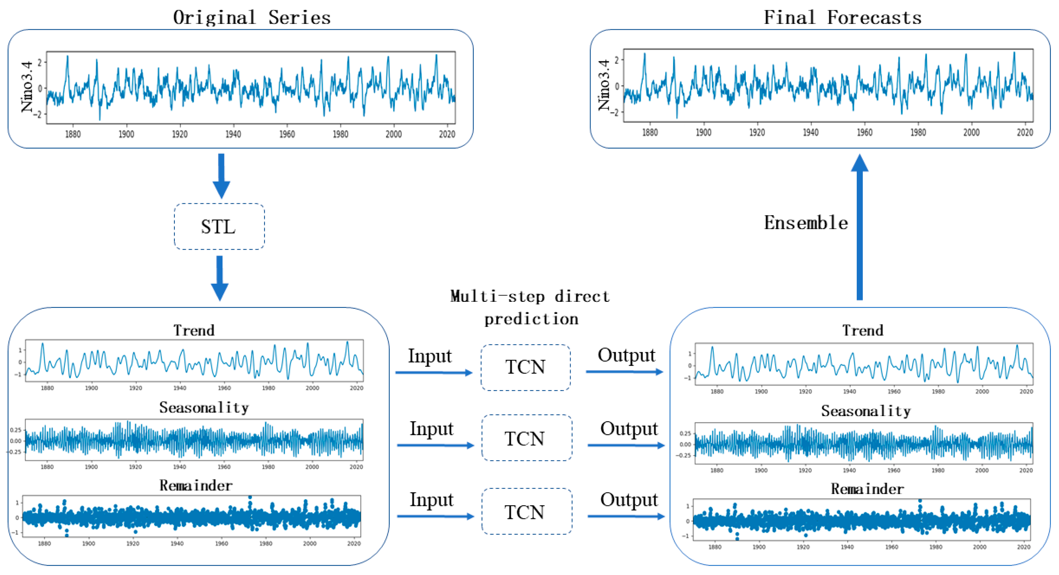
The STL-TCN model combines STL and TCN. The Niño 3.4 index is decomposed into simpler and meaningful components via STL. This helps the TCN to capture the trend, cyclical and seasonal features in the series, which in turn improves the forecast accuracy. The specific steps are as follows:
The Niño 3.4 index is decomposed into the trend component , seasonal component and remainder component by STL.
Normalize the three components.
Prediction of each of these three components using TCN neural network.
The trend component forecast, seasonal component forecast, and residual component forecast of Niño 3.4 index will be inverse normalized and summed to obtain the final Niño 3.4 forecast, The detailed process can be seen in
Figure 4.
In this experiment the whole data set is divided into training and test sets according to the ratio of 8:2. The specific division is shown in
Table 1.
The model consists of STL, TCN layers, and a fully connected layer. The main hyperparameters of TCN include the size of the convolutional kernel, dilation factors, and the number of convolutional kernels. In this study, the hyperparameters for TCN are set as follows: the one-dimensional convolutional kernel size is set to 7; the dilation factors are sequentially set to 1, 2, and 4; the residual modules consist of three layers, and the number of convolutional kernels in each layer is set to 128, 64, and 32, respectively; and the dropout parameter is set to 0.2. The optimizer used is the Adam algorithm, with a learning rate of 0.001. The maximum number of training epochs is set to 20, the batch size is set to 4, and the random seed is fixed.
2.6. Evaluation Metrics
To evaluate the model’s performance, the following three evaluation metrics were selected in this study. (1) Root mean square error (RMSE). (2) Mean absolute error (MAE). (3) Pearson correlation coefficient (PCC). The calculation formulae are as follows:
represents the observed value (true value); represents the predicted value; and are the averages of and concernino , respectively.
3. Results and Discussion
3.1. Models Are Trained Using Different Time Windows
The time window refers to the duration of past observed values considered when predicting future data points. Selecting an appropriate time window is crucial for the performance of prediction models in many forecasting problems. If the time window is too short, the model might fail to capture long-term trends and patterns, thus limiting its predictive capabilities. On the other hand, if the time window is too long, the model may capture excessive historical information, including noise and irrelevant details, that do not hold representativeness for future predictions, thereby affecting the generalization of the model’s performance. Therefore, it is essential to carefully choose the time window, considering the characteristics of the data and the forecasting objectives, to achieve optimal predictive performance.
Predicting the Niño 3.4 index is a typical task in time series forecasting. The time window within a time series model has a significant impact on its performance, as it directly affects the structure of the temporal data and consequently influences the model’s training and performance. To determine the optimal time window, this study varied the time window of the model and evaluated its performance. The time windows were increased by intervals of 3 months, ranging from 3 to 36. Specifically, the following time windows were tested: {3, 6, 9, 12, 15, 18, 21, 24, 27, 30, 33, 36}. These time windows were used to train the model, and performance metrics such as PCC, RMSE, and MAE were computed.
Table 2 presents the predictive performance of different time windows for a 12-month lead time. It can be observed that when the time window is 12 months, the PCC reaches its highest value of 0.62, while the RMSE and MAE reach their lowest values of 0.70 °C and 0.55 °C, respectively. In contrast, the predictive performance is poorer when the time window is 3 months. This indicates that shorter time windows may not provide sufficient information for forecasting long-term sequences, making it challenging for the model to capture effective periodic and seasonal features. From
Figure 5, it can be seen that as the time window exceeds 12 months, the errors increase while the correlation coefficients decrease, resulting in a deterioration of the model’s predictive performance. This suggests that a larger time window is not necessarily better. Therefore, when predicting the Niño 3.4 index, a time window of 12 months is most suitable.
3.2. Comparison and Analysis of Different Models
To verify the accuracy and validity of the prediction model proposed in this paper, other more commonly used models were constructed for comparison experiments, specifically the gate recurrent unit (GRU), multiple layer perception (MLP), LSTM, TCN and STL-LSTM.
Figure 6 illustrates the variations in PCC, RMSE, and MAE metrics for different models when forecasting the Niño 3.4 index ahead by 1–24 months, while
Table 3 presents detailed results for selected months. From the figure, it can be observed that as the lead time increases, the predictive performance of all models tends to decline. At a lead time of one month, the correlation coefficient metrics for all models are quite similar, with STL-TCN slightly higher. However, except for the STL-TCN and STL-LSTM models, the predictive performance of the remaining models rapidly deteriorates, providing effective forecasts for only about six months. The STL-TCN model achieves the longest effective forecasting period, followed by the STL-LSTM model.
Overall, the STL-TCN model exhibits the best predictive performance with the lowest being the RMSE and MAE. The MLP model performs relatively poorly, which demonstrates the weaker ability of traditional feed-forward neural networks, such as MLP, in handling temporal relationships. TCN, on the other hand, excels at capturing long-term dependencies in the data, leading to better performance. Both LSTM and GRU demonstrate similar predictive performance, although GRU has fewer parameters. However, based on correlation coefficient indicators, the basic GRU model slightly underperforms compared to the basic LSTM model. The STL-TCN model shows a significant improvement in predictive performance compared to the TCN model, and, similarly, the STL-LSTM model exhibits notable enhancements over the LSTM model. These findings indicate that applying STL to extract components such as trend, seasonality, and residuals effectively reduces the inter-component interactions and contributes to improving the accuracy of multi-step predictions.
To further explore the impact of different decomposed sequences on predictive performance, we conducted predictions for each sequence and present the results in
Figure 7d, illustrating the decomposed trend component (T), seasonal component (S) and residual component (R). By comparing the prediction results of each component, we can better understand their contributions to the final prediction of the Niño 3.4 index. Based on the results, we can observe that the seasonal component exhibits the best prediction performance. This may be attributed to its regular and periodic nature, which makes it easier to predict. The results of the trend component exhibit the closest similarity to the final forecasting results of the Niño 3.4. The remainder component is also known as the noise or the residuals of the decomposition. It contains the random fluctuations, measurement errors, or other factors that cannot be attributed to the underlying trend or seasonal effects. These unpredictable elements make it challenging to capture their future behavior accurately.
Figure 7a–d show the predicted Niño 3.4 index results of the STL-TCN model 1, 3, 6, and 12 months in advance, respectively. As can be seen from the figures, all the predicted Niño 3.4 index curves are basically consistent with the actual curves in terms of growth trends and turning points, indicating that the model can effectively capture the time series variation characteristics of the Niño 3.4 index. The curve obtained by forecasting one month in advance has the highest degree of overlap with the actual Niño 3.4 index curve, with a PCC of 0.97, indicating a strong linear correlation between the predicted and actual values; and an RMSE of 0.20 °C and MAE of 0.16 °C indicate relatively small forecasting errors. However, with the increase in the prediction time, the fluctuation of the predicted value gradually decreases and a lag phenomenon appears. This phenomenon may stem from the increased uncertainty due to the increase in forecast length. The lowest match between the forecast results and the actual value curve is found 12 months ahead of time, with the PCC dropping to 0.62, RMSE increasing to 0.70 °C and MAE increasing to 0.55 °C, indicating an increase in forecast error.
3.3. ENSO Event Prediction and Analysis
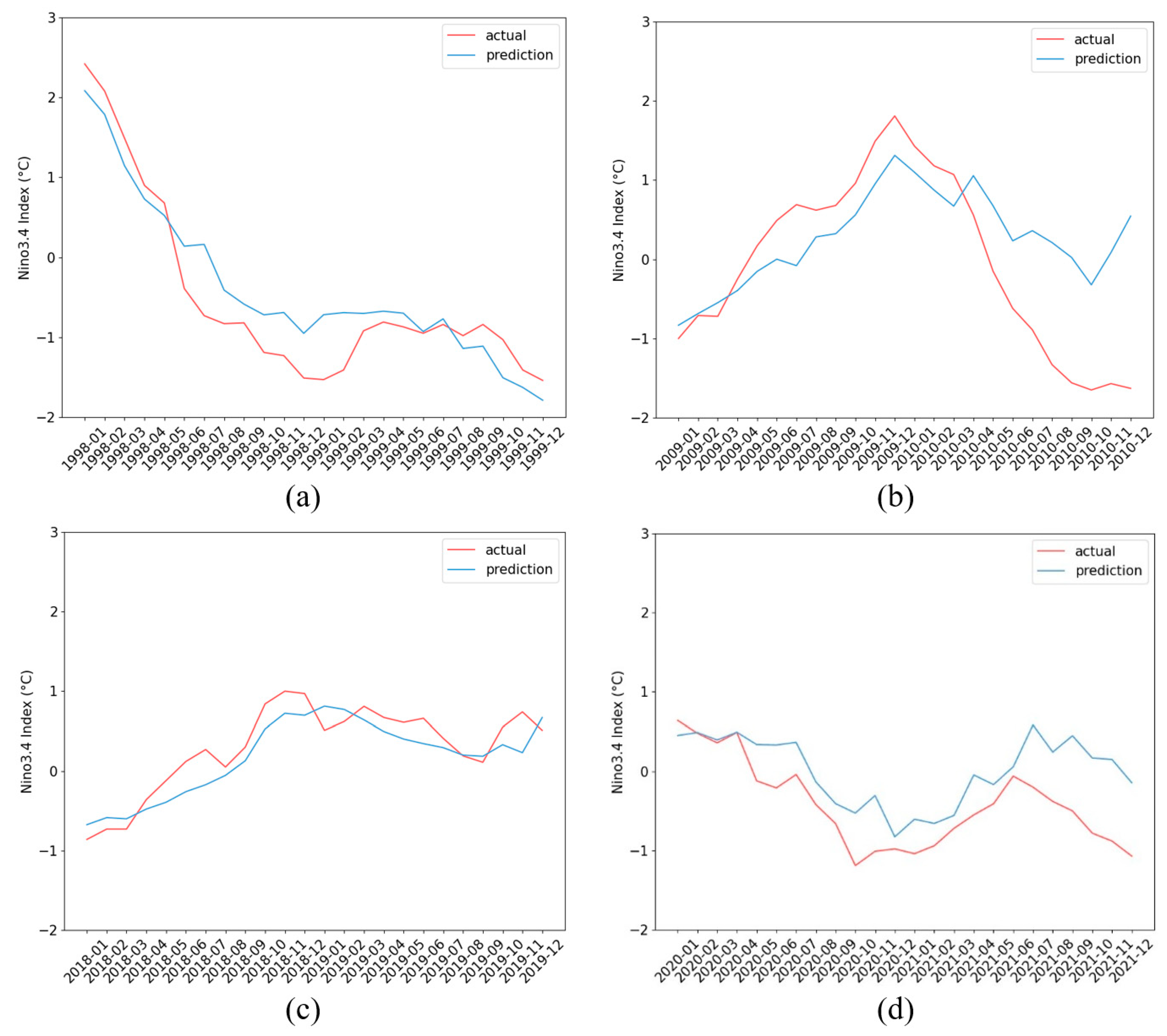
To further validate the prediction effectiveness of the STL-TCN model for ENSO events, the model was used to predict ENSO events in 1998/1999, 2009/2010, 2018/2019, and 2020/2021. As can be seen in
Figure 8 the STL-TCN model more accurately predicts ENSO events of significant scale in 1997/1998, and ENSO events of moderate scale in 2018/2019 and 2020/2021. In all three events, the model can better simulate the development process, intensity and duration of the events, proving its strength in capturing the dynamic characteristics of ENSO. For the 2009/2010 ENSO event, the STL-TCN model performs better in predicting the peak of the El Niño event; however, the prediction decreases in the subsequent La Niña phase. The model fails to accurately simulate the development of the La Niña event after 14 months, showing a trend opposite to the actual situation. In summary, the STL-TCN model shows better results in predicting ENSO events of different intensities, especially in capturing event trends and peak intensities, and provides an effective tool for ENSO event studies.
4. Conclusions
This paper presents a novel hybrid model that combines the STL decomposition algorithm and the TCN model for Niño 3.4 index prediction. Taking RMSE, MAE, and R as the evaluation indicators of prediction accuracy, through experimental verification and comparative analysis, the following conclusions are drawn:
Combining the STL time series decomposition method and the TCN model, the cumulative error of long time series forecasting can be significantly reduced, and the forecasting accuracy can be greatly improved at the same time.
Compared with the popular LSTM, the STL-TCN model performs better and has better prediction results.
The STL-TCN model can effectively forecast the ENSO events in 1998/1999, 2009/2010, 2018/2019 and 2020/2021, and the prediction results of these events can fit the fluctuations and trends of their changes well.
In this study, the Niño 3.4 index was selected as the object for time series prediction, but ENSO also contains other indices. Therefore, applying model migration learning to other relevant ENSO indices for prediction can be considered in the future.


