Fishing Behavior Detection and Analysis of Squid Fishing Vessel Based on Multiscale Trajectory Characteristics

Abstract

Accurate fishing activity detection from the trajectories of fishing vessels can not only achieve high-precision fishery management but also ensure the reasonable and sustainable development of marine fishery resources. This paper proposes a new method to detect fishing vessels’ fishing activities based on the defined local dynamic parameters and global statistical characteristics of vessel trajectories. On a local scale, the stop points and points of interest (POIs) in the vessel trajectory are extracted. Voyage extraction can then be conducted on this basis. After that, multiple characteristics based on motion and morphology on a global scale are defined to construct a logistic regression model for fishing behavior detection. To verify the effectiveness and feasibility of the method, vessel trajectory data, and fishing log data collected from Chinese ocean squid fishing vessels in Argentine waters in 2020 are integrated for fishing operation detection. Multiple evaluation metrics show that the proposed method can provide robust and accurate recognition results. Moreover, further analysis of the temporal and spatial distribution and seasonal changes in squid fishing activities in Argentine waters has been performed. A more refined assessment of the fishing activities of individual fishing vessels can also be provided quantitatively. All the results above can benefit the regulation of fishing activities.

1. Introduction

The local environment will be severely harmed by overfishing and overuse of marine resources [1], which will have an impact on how nearby communities and the global community are developed and how food chains are supplied [2]. Overfishing, which is mostly caused by illicit, unreported, and unregulated (IUU) fishing [3], is the principal cause of the depletion of marine fisheries resources. IUU fishing is a widespread global phenomenon that not only endangers the existence of threatened fish populations and pollutes the ocean with microplastic [4], but it is also a transnational crime [5]. Severe damage to a nation’s marine rights, resource development, and sustainable development of marine fish is posed by the decline and scarcity of marine resources, which frequently lead to disputes between fishing fleets of different countries over marine fishery resources [6,7]. Diverse, relevant conservation policies have been put in place to ensure the healthy and sustainable growth of regional and global fisheries as marine fisheries receive more attention globally [8]. The growth of people’s livelihoods and ecological protection need to be taken into account when formulating policies since some permanent fishing ban regulations have overlooked the influence on the livelihood of fishermen’s families [9]. In order to support the creation of fishery policies, assure the healthy and sustainable development of fisheries [10], and achieve high-precision fishery management [11], information technology must be used.

The demands for fisheries management mainly include tracking the activity footprint of fishing vessels [12], evaluating fishing efforts, and regulating illegal fishing [5]. Many studies still rely on survey techniques and mathematical models for estimation [13,14], but when fishing locations are numerous and dispersed throughout the vast open sea, it may be impractical to rely solely on on-site law enforcement [15], particularly during the COVID-19 pandemic, which exacerbated illegal fishing activities [16]. The Automatic Identification System (AIS) was originally designed as a navigational safety tool to avoid collisions [17]. Due to its ability to record information, such as the real-time position and speed of a ship, AIS is now widely used for the regulation of ship traffic. The question of how to automatically identify fishing operations on fishing vessels using AIS data has grown in importance.

Most studies employ a coarse-grained speed threshold to determine the operational status of the vessel because the speed range that the fishing vessel maintains during fishing operations is lower than that during normal sailing [18]. As fishing vessels are subject to special navigation legislation, statistical analysis of the speed distribution that follows a bimodal distribution can be used to precisely determine the speed distribution in the AIS data of fishing vessels [19]. By splitting the speed range of fishing vessels, statistical results can increase detection accuracy, but they still fall short of more complex requirements for fishery management. Recently, researchers started using machine learning techniques to refine the detection model based on the distribution of fishing vessel speed [20,21]. This is due to the rapid growth of machine learning and artificial neural networks. A number of multi-feature models based on AIS trajectory points are also suggested to further increase detection accuracy [22,23,24].

In the above studies, the feature construction between individual track points or continuous track points is used to determine whether a certain track point belongs to fishing activities. The point-by-point detection method has limitations, as some high-speed track points in fishing activities may be misjudged as non-fishing points, and some low-speed track points in normal sailing activities may be misjudged as fishing trajectory points. Moreover, the detection results of the above methods cannot obtain complete spatiotemporal information for each independent fishing behavior, so they cannot provide accurate data support for fisheries management and fishing activity regulation. This article takes squid fishing vessels as an example and proposes a new fishing behavior detection method based on AIS data. By combining the local dynamic parameters and global statistical characteristics of trajectories defined in this paper, the traditional sliding window algorithm is optimized, a candidate fishing trajectory extraction method based on POI is proposed, and a discriminative model of fishing behavior based on logical regression is proposed. Compared with the point-by-point detection model, the recognition results are transformed from a single point to a trajectory segment, which improves the transparency and traceability of fishing activities and can prevent the reduction in detection accuracy caused by some solitary locations during fishing operations.

The rest of the article is structured as follows: Multiscale trajectory characteristics of squid fishing vessels are described in Section 2. In Section 3, the specific models and procedures for identifying fishing behavior and calculating fishing effort are described. The AIS data of squid fishing vessels in Argentinean waters are analyzed using the proposed model and method in Section 4, which also presents a summary of the detailed information on individual fishing activities of fishing vessels and the overall distribution of spatial and temporal characteristics of fishing activities over the course of the year. In Section 4, the main conclusions are finally presented.

2. Multiscale Trajectory Characteristics of Squid Fishing Vessels

A fishing vessel’s trajectory carries a number of useful properties, including Maritime Mobile Service Identity (MMSI), longitude, latitude, speed over ground, course over ground, etc. In this paper, the AIS data has been parsed, so the timestamp is also important information in the subsequent study. A fishing vessel’s trajectory characteristics change depending on whether it is actively fishing. Even though fishing vessels have different operation types, when they are fishing, they will frequently change their course and speed [25]. Therefore, changes in local dynamic parameters and global statistical characteristics can reflect the characteristics of fishing activities.

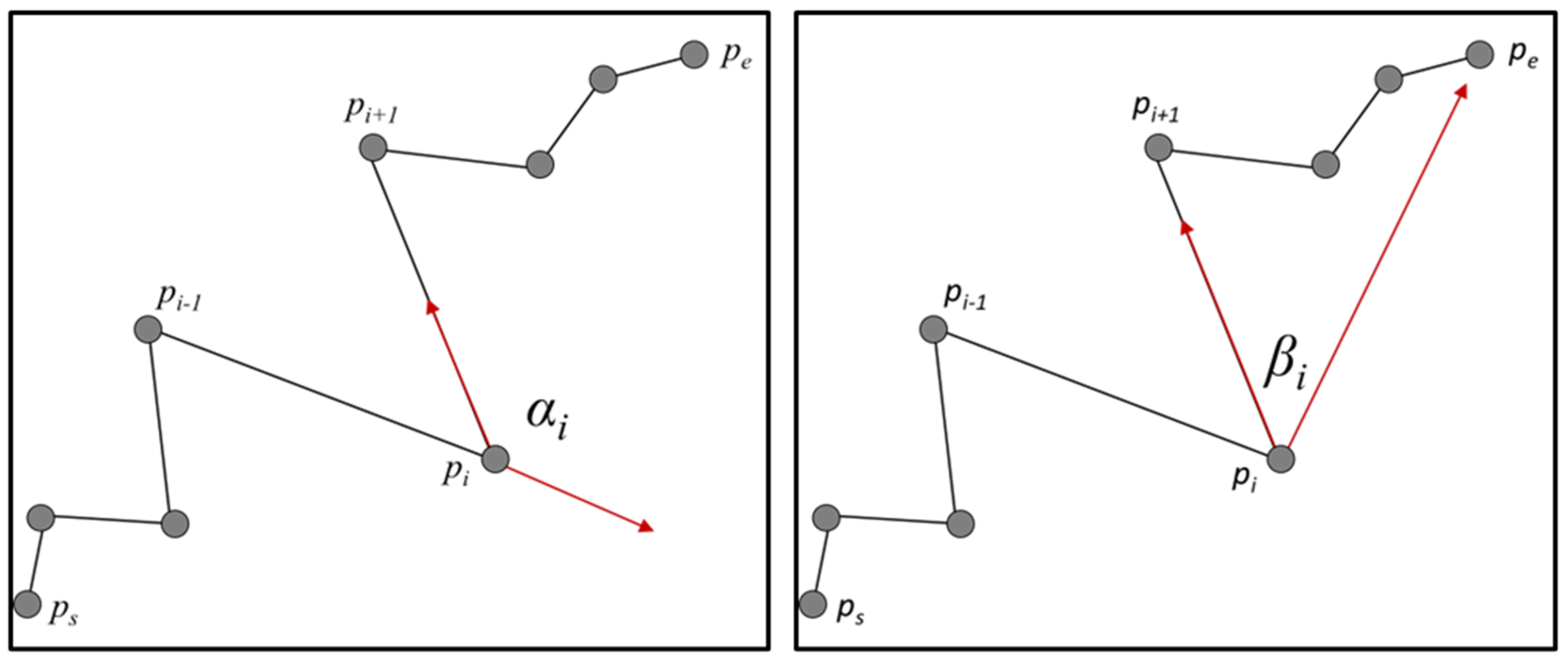
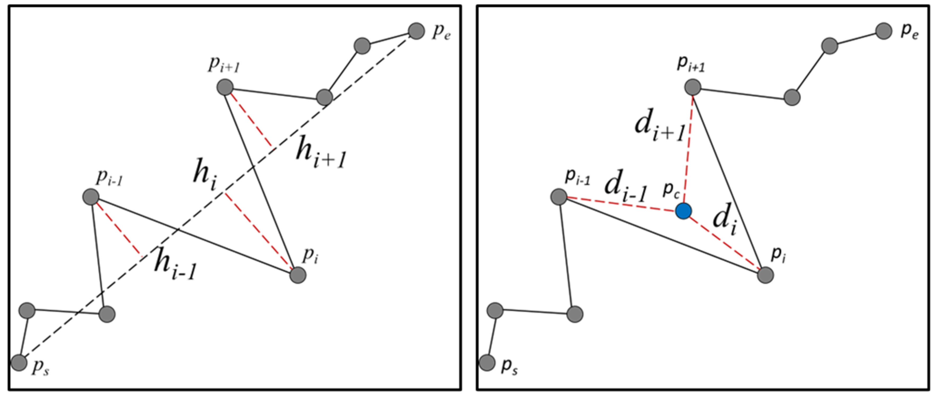
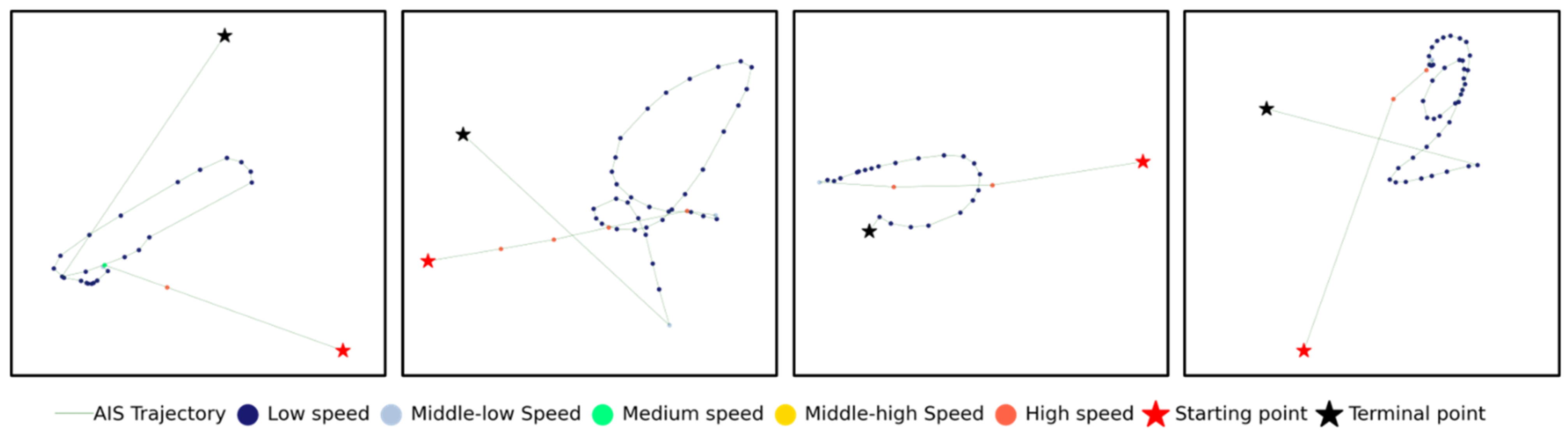
2.1. Local Dynamic Parameters of Squid Fishing Vessel

The collection of all fishing vessel trajectories is denoted by $T_{AIS}=\left\{T_1,\dots ,T_m,\dots ,T_M\right\}$, where m represents different fishing vessels, and M is the total number of all fishing vessels. The equivalent trajectory for fishing vessel m can be written as $T_m=\left\{p_1,\dots ,p_i,\dots p_N\right\}$, where N is the number of discrete track points in the AIS trajectory. Each trajectory point $p_i$ contains the ship’s motion and spatial parameters, which are written as $p_i=\left\{lo{n}_i,la{t}_i,ut{c}_i,v_i,c_i\right\}$. These parameters are the fishing vessel’s longitude and latitude coordinates ($lo{n}_i,la{t}_i$), timestamp ($ut{c}_i$), speed over ground ($v_i$), and course over ground ($c_i$). More local dynamic parameters can be discovered by examining the spatiotemporal relationships between consecutive track points.

Latitude and longitude coordinates and a timestamp can be first used to establish the time step $\Delta utc$ and space step $\Delta d$ between two discrete track locations. The semi-positive vector formula is used to calculate the geospatial distance between two consecutive track points.

$$\Delta d_i=d\left(p_i,p_{i+1}\right)=2R{\sin }^{-1}\left(\sqrt{{\sin }^2\left(\frac{la{t}_{{}_{i+1}}-la{t}_i}{2}\right)+\cos \left(la{t}_{i+1}\right)\cos \left(la{t}_i\right){\sin }^2\left(\frac{lo{n}_{{}_{i+1}}-lo{n}_i}{2}\right)}\right)$$

(1)

$$\Delta ut{c}_i=ut{c}_{i+1}-ut{c}_i$$

(2)

where $p_i$ and $p_{i+1}$ represent two consecutive track points, respectively. $R$ stands for the earth’s radius (6.3771 × 10⁶ m), $utc$ represents the reported timestamp corresponding to the track point, and $lon$ and $lat$ are the longitude and latitude in the WGS-84 coordinate system.

By combining these factors with fishing vessel velocity, it is possible to further determine the velocity differential $\Delta v$ and acceleration $a$.

$$\Delta v_i=v_{i+1}-v_i$$

(3)

$$a_i=\frac{\Delta v_i}{\Delta ut{c}_i}$$

(4)

The position information in the AIS data uses the WGS-84 coordinate system, which is a geocentric spatial right-angle coordinate system. The WGS-84 coordinate system is converted to Mercator projection coordinates in order to calculate the vector angle between two successive track points because the WGS-84 coordinate system is not an equiangular coordinate system. The transformational formula is as follows.

$$\left\{\begin{array}{c}{x}_m=\frac{\pi R\times lon}{180}\\ y_m=R\times \ln \left(\tan \left(\frac{\pi }{4}+\frac{\pi lat}{360}\right)\right)\end{array}\right.$$

(5)

where $x_m$ and $y_m$ are the longitude and latitude in the Mercator projection coordinate system.

Due to significant course loss and significant AIS inaccuracy, the turning angle is defined and calculated when the longitude and latitude coordinates are converted into the Mercator projection coordinates. The consecutive track points, $p_{i-1}$, $p_i$, and $p_{i+1}$ denoted as gray circles in Figure 1 form two adjacent track segments. Two vectors, $p_{i-1}$ pointing to $p_i$, and $p_i$ pointing to $p_{i+1}$, make up the turning angle ${\alpha }_i$ for $p_i$. The formula for the solution is as follows:

$${\alpha }_i={\cos }^{-1}\left(\frac{\stackrel{\rightharpoonup }{p_{i-1}{p}_i}\times \stackrel{\rightharpoonup }{p_i{p}_{i+1}}}{\stackrel{\rightharpoonup }{\left|p_{i-1}{p}_i\right|}\times \stackrel{\rightharpoonup }{\left|p_i{p}_{i+1}\right|}}\right)$$

(6)

At the same time, in order to reflect the spatial relationship between the navigation direction of each track point and the final destination, we define the directional error angle $\beta$ of each trajectory point. As shown in Figure 1, the directional error angle ${\beta }_i$ for each track point $p_i$ is composed of two vectors, $p_i$ pointing to $p_e$, and $p_i$ pointing to $p_{i+1}$. The formula for the solution is as follows:

$${\beta }_i={\cos }^{-1}\left(\frac{\stackrel{\rightharpoonup }{p_i{p}_e}\times \stackrel{\rightharpoonup }{p_i{p}_{i+1}}}{\stackrel{\rightharpoonup }{\left|p_i{p}_e\right|}\times \stackrel{\rightharpoonup }{\left|p_i{p}_{i+1}\right|}}\right)$$

(7)

where $p_e$ represents the last track point of the trajectory segment.

To reflect the relative position relationship between each track point and the starting and ending line of the entire trajectory, we define the distance between each track point and the starting and ending line of the entire trajectory, called the centerline distance $h_i$. The related diagram is shown in Figure 2, and the solution formula is as follows:

$$h_i=\frac{\stackrel{\rightharpoonup }{p_i{p}_s}\times \stackrel{\rightharpoonup }{p_i{p}_e}}{d\left(p_s,p_e\right)}$$

(8)

where $d\left(p_s,p_e\right)$ represents the geographic distance between the starting and ending points of the trajectory, and $\stackrel{\rightharpoonup }{p_i{p}_s}$ and $\stackrel{\rightharpoonup }{p_i{p}_e}$ represent two vectors of track point $p_i$ pointing towards the starting and ending points of the trajectory, respectively.

Finally, in order to reflect the relative position relationship of each trajectory point to the entire trajectory center point, we defined the center distance $d_{\mathrm{c},\mathrm{i}}$ of each trajectory point $p_i$. As shown in Figure 2, the formula for calculating the coordinates of the geometric center point of the trajectory segment and the center distance of each track point is as follows:

$$\left\{\begin{array}{c}lo{n}_c=\frac{1}{n}{\displaystyle \sum _{i=1}^{n}lo{n}_i}\\ la{t}_c=\frac{1}{n}{\displaystyle \sum _{i=1}^{n}la{t}_i}\end{array}\right.$$

(9)

$$d_{\mathrm{c},\mathrm{i}}=d\left(p_i,p_c\right)=2R{\sin }^{-1}\left(\sqrt{{\sin }^2\left(\frac{la{t}_c-la{t}_i}{2}\right)+\cos \left(la{t}_c\right)\cos \left(la{t}_i\right){\sin }^2\left(\frac{lo{n}_c-lo{n}_i}{2}\right)}\right)$$

(10)

By analyzing the local spatiotemporal features of trajectories, we can extract valuable information from each track point. This information can be expressed as a set, denoted as $P_i$, which includes longitude ($lo{n}_i$), latitude ($la{t}_i$), timestamp ($ut{c}_i$), velocity ($v_i$), course over ground ($co{g}_i$), time step ($\Delta ut{c}_i$), space step ($\Delta d_i$), velocity differential ($\Delta v_i$), acceleration ($a_i$), turning angle (${\alpha }_i$), direction error angle (${\beta }_i$), centerline distance ($h_i$), and center distance ($d_{c,i}$).

$$P_i=\left\{lo{n}_i,la{t}_i,ut{c}_i,v_i,co{g}_i,\Delta ut{c}_i,\Delta d_i,\Delta v_i,a_i,{\alpha }_i,{\beta }_i,h_i,d_{c,i}\right\}$$

(11)

The trajectory local dynamic parameters mining method takes into account not only the spatiotemporal relationship between continuous track points but also the relationship between each point and important spatial nodes of the overall trajectory. This approach captures both the instantaneous changes in ship motion parameters over a short period and the spatial position of each point relative to the entire segmented trajectory.

Through further statistical calculation methods, it becomes feasible to develop global trajectory characteristic models and conduct pattern mining of squid fishing vessel behavior in subsequent analyses.

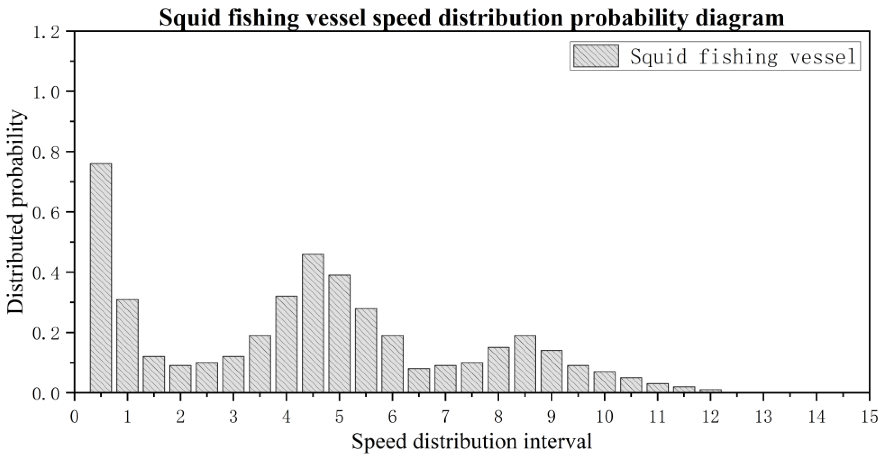
2.2. Global Statistical Characteristics of Squid Fishing Vessel

By observing the fishing vessel during its transition from normal sailing to fishing, we can observe significant changes in its trajectory. Figure 3, Figure 4 and Figure 5 depict how fishing vessels experience changes in their dynamic parameters, such as a decrease in speed and fluctuations in the course, and changes in their trajectory morphology. As a result, we have defined two types of global statistical characteristics to describe fishing trajectories, taking into account both motion and morphology perspectives.

At this juncture, we can represent the set of trajectory points for a potential fishing trajectory in the following manner:

$$T=\left\{p_1,p_2,\dots ,p_i,\dots ,p_n\right\}$$

(12)

Figure 3 and Figure 4 show the variations in velocity and turning angle in the trajectories of a squid fishing vessel’s sea fishing voyage. Based on the start time of squid fishing recorded in the fishing vessel log, we found that the velocity of the squid fishing vessel during normal sailing is maintained at an economical speed with little the change in course; during fishing, the speed is mostly at a low level, and the change in course is more pronounced.

To begin with, two motion statistical characteristics are specified, namely, the proportion of low-velocity and the proportion of course fluctuation, to quantify the amplitude of speed and course fluctuation of the fishing trajectory.

Proportion of low-velocity: is the proportion of track points with low speed in the trajectory $T$, denoted as $P_v$. The method of computation is as follows.

$$P_v=\frac{card\left(\left\{v_i\left|\left(v_i\in T\right)\cap \left(v_i\le v_{\epsilon }\right)\right.\right\}\right)}{card\left(T\right)}$$

(13)

In Equation (13), $card\left(\right)$ is the function for solving the number of elements in the corresponding set; $v_{\epsilon }$ is a low-speed threshold that has been established and $P_v$ is the proportion of low-speed track points in the trajectory $T$.

Proportion of course-fluctuation: is the proportion of turning track points in the trajectory $T$, denoted as $P_{\alpha }$. The method of computation is as follows:

$$P_{\alpha }=\frac{card\left(\left\{{\alpha }_i\left|\left({\alpha }_i\in T\right)\cap \left({\alpha }_i\le {\alpha }_{\epsilon }\right)\right.\right\}\right)}{card\left(T\right)}$$

(14)

where ${\alpha }_{\epsilon }$ is a turning angle threshold that has been established and $P_{\alpha }$ is the proportion of turning track points in the trajectory $T$.

Figure 5 visualizes the fishing trajectory of the squid fishing vessel. Compared to normal sailing trajectories, fishing trajectories have the following characteristics: (1) forming a more concentrated cluster of track points within a narrower spatial range; (2) the purpose of navigation is not clear enough; (3) the trajectory has a higher degree of twists and turns; and (4) navigation efficiency is lower.

Four morphological statistical characteristics, namely, cohesion, sinuosity, straightness, and navigation efficiency, were specified to quantify the above four features of the fishing trajectory.

Cohesion: measures the variance in the distance between each track point and the center of the trajectory $T$ denoted as $c_T$. The method of computation is as follows:

$$c_T=\sqrt{\frac{1}{n}\left({\displaystyle \sum _{i=1}^n{\left(d_{c,i}-\frac{1}{n}{\displaystyle \sum _{i=1}^n{d}_{c,i}}\right)}^2}\right)}$$

(15)

In Equation (15), $d_{c,i}$ is the geographic distance between each track point and the center point of the trajectory $T$. This statistical indicator reflects the degree of concentration of all track points in the geographic space of the trajectory.

While fishing, the fishing vessel makes more twists, which causes a more convoluted trajectory. In order to distinguish between fishing and regular sailing, sinuosity, and straightness are defined.

Sinuosity: is the average distance between each track point’s centerline distance $h_i$, denoted as $sinuosit{y}_T$. The method of computation is as follows:

$$sinuosit{y}_T=\frac{1}{n}{\displaystyle \sum _{i=1}^n{h}_i}$$

(16)

This statistical indicator reflects the degree of twists and turns in the trajectory.

Straightness: is the average cosine of each track point’s direction error ${\beta }_i$, denoted as $straightnes{s}_T$. The method of computation is as follows:

$$straightnes{s}_T=\frac{1}{n}{\displaystyle \sum _{i=1}^n\cos {\beta }_i}$$

(17)

This statistical indicator reflects whether the navigation purpose of the trajectory is clear.

Navigation efficiency: is the ratio of the distance between the starting and finishing points of the trajectory to the overall distance covered by the trajectory. The formula for calculation is as follows:

$$efficienc{y}_T=\frac{d\left(p_s,p_e\right)}{{\displaystyle \sum _{i=1}^{n-1}d\left(p_i,p_{i+1}\right)}}$$

(18)

In Equation (18), $d\left(p_s,p_e\right)$ is the geographic distance between the starting and ending points of the trajectory, ${\displaystyle \sum _{i=1}^{n-1}d\left(p_i,p_{i+1}\right)}$ is the navigation mileage of the trajectory. This statistical indicator reflects the navigation efficiency of the trajectory.

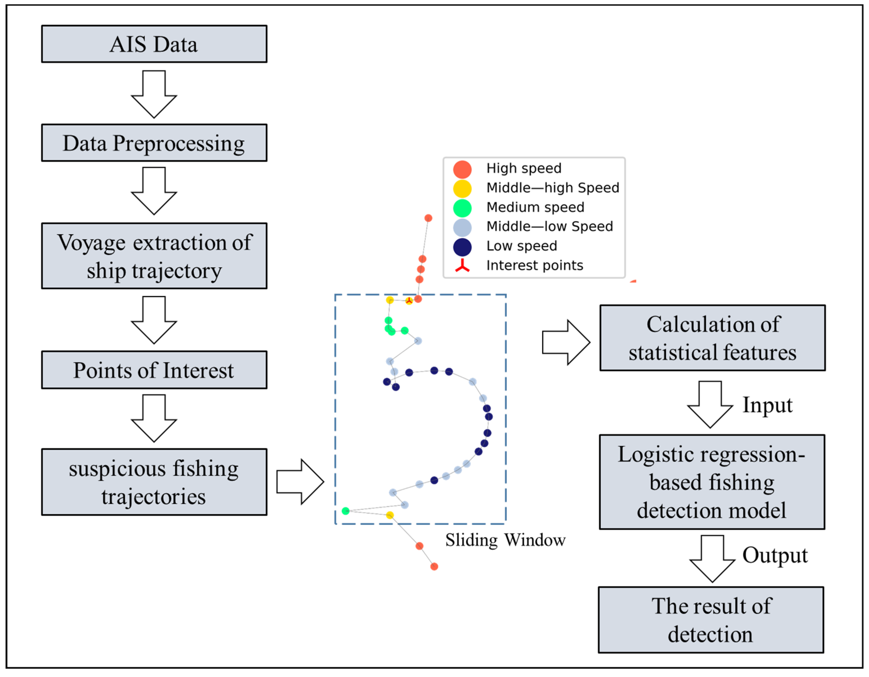
3. Detection Method of Fishing Behavior Based on Trajectory Characteristics

Before fishing behavior detection, track quality inspection should be completed since false alerts and missing track points can be found in real AIS data. First, the abnormalities in parameters, such as longitude, latitude, speed, acceleration, and direction, in the AIS data will be identified and fixed [26]. It is of little importance to determine the fishing behavior of fishing vessels in locations with major missing track points because a fishing activity typically lasts for 3 to 15 h. In this study, the boxplot method’s use of the interquartile range to identify outliers is utilized. First, determine the top and lower quartiles of the time difference between two successive points on a ship’s trajectory by measuring and counting the time difference. The time threshold for detecting missing AIS data is therefore defined as the top thousandth point of the box plot plus 1.5 times the difference between the upper thousandth point and the lower thousandth point. It is considered that AIS data is significantly deficient whenever the time difference between two track locations exceeds the time threshold or the minimum fishing time, which is generally set at 3 h.

As shown in Figure 6, the workflow of the fishing behavior detection algorithm is as follows:

• Input the AIS trajectory of fishing vessels, and the trajectory is preprocessed.
• Use a density-based clustering iterative approach to extract the center point coordinates of fishing ports. Based on this, the single voyage trajectory is divided.
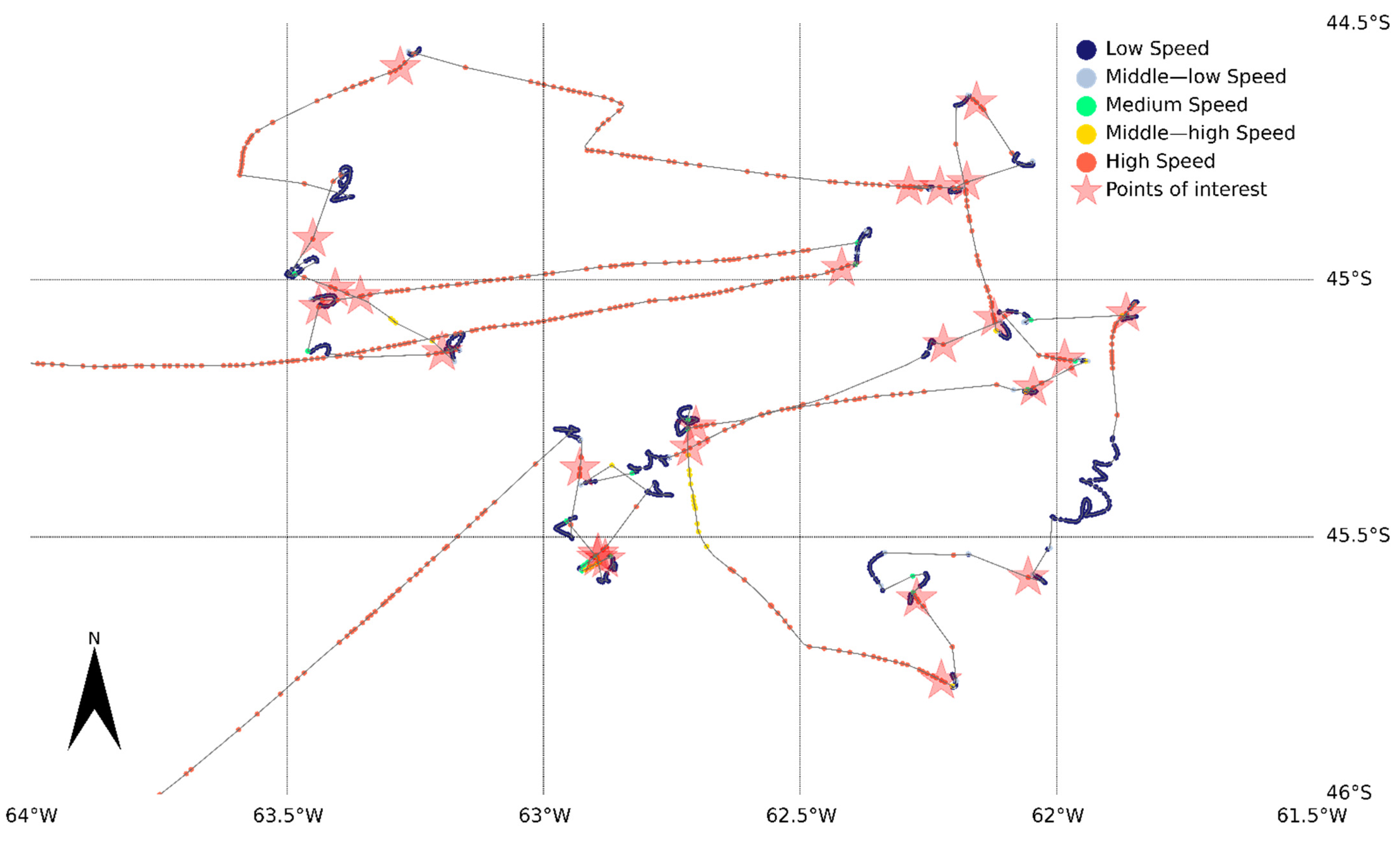
• Traverse every voyage’s trajectory. If there are POI that change from high speed to low speed, take all POI as the starting point of the sliding window.
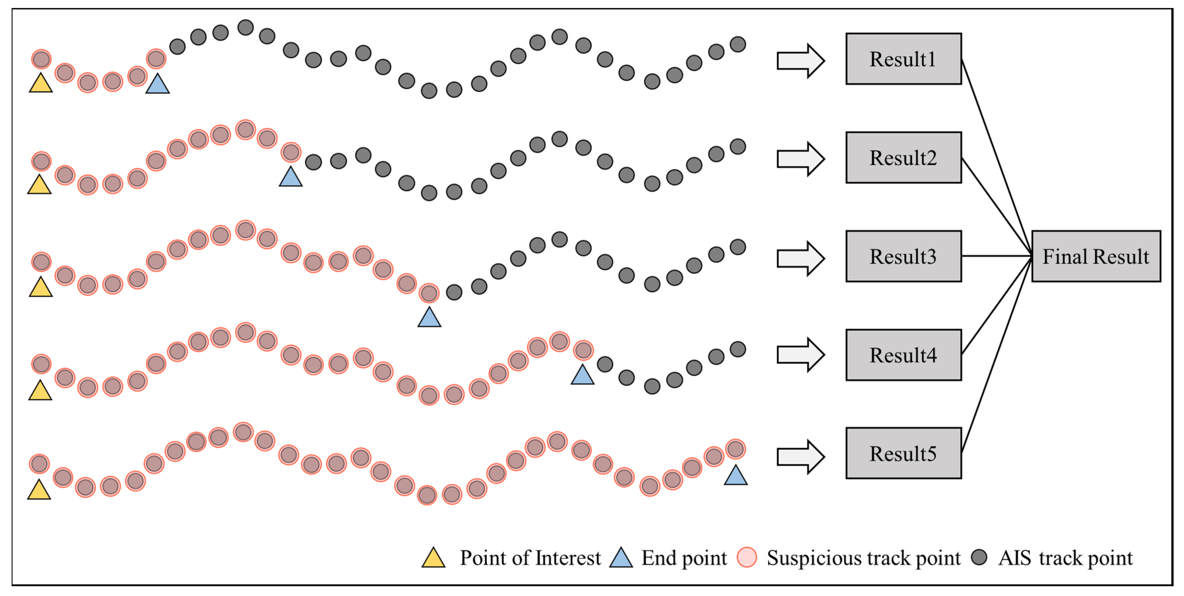
• Starting from each POI, the minimum time length of the sliding window is determined by the shortest fishing time and the minimum number of track points. The sliding window is extended every half hour, and the trajectory within the window will be considered a suspicious fishing trajectory.
• Extract six global statistical characteristics defined in this paper from the suspicious fishing trajectories, including proportion of low-velocity, proportion of course-fluctuation, direction constancy, cohesion, sinuosity, straightness, and navigation efficiency.
• Use the logistic regression model trained by the training samples to distinguish whether the suspicious fishing trajectory is a fishing trajectory. Select the trajectory with the highest probability as the final fishing trajectory.

3.1. Voyage Trajectory Extraction

Squid fishing is primarily completed in one of two ways in the Argentinean seas. One spends a few days fishing, then returns to port to relax on rest days. Another one goes an entire year without returning to port while fishing. A fishing vessel’s trajectory could consist of a lengthy, intricate geometric path with a variety of mobility patterns. Some of the fishing vessels operating on the high seas are engaged in fishing operations at sea all year round and hand over to transshipment vessels after the catch is full and do not return to the fishing port to deal with the catch, so the movement mode is mainly divided into two states of fishing and normal sailing; however, the movement mode of most fishing vessels is mainly divided into three states of fishing port anchor, fishing, and normal sailing.

The “Stop-Move” conceptual model is first employed to separate the raw ship trajectory into a collection of stops and a set of continuous sub-trajectories between stops for the purpose of detecting fishing activity. Mobility patterns for sailing and fishing between various anchorages may be present in each sub-trajectory. In this paper, a density-based clustering iterative approach is used to swiftly recover fishing vessel stops from a large number of AIS track points. First, any track locations in the AIS data that had a velocity of less than 0.5 knots were filtered out and treated as stop points [27]. A few stops within a short period of time during the process of fishing vessels leaving the port can be classified as noise spots since the stop points in the port are more intensive in general. In the process of stop point clustering, the first iteration allows for the extraction of the longitude and latitude coordinates of the central point and the berthing area of a single ship. The berthing areas of several ships may be found in the second iteration, and center locations’ longitude and latitude coordinates can be gleaned. The anchorages’ longitude and latitude coordinates are then obtained in the third iteration. The raw AIS trajectory of each vessel can be divided by the anchorage to get the single voyage sub-trajectory, as shown in Figure 7.

3.2. Suspicious Fishing Trajectory Extraction Based on Variable Length Sliding Window

The fishing behavior defined in this paper is the trajectory segment produced by the fishing activities of fishing vessels. In order to detect the fishing behavior of fishing vessels from their voyage sub-trajectories, this paper proposes a two-staged detection method. The initial phase involves identifying possible fishing trajectory segments that are called candidate fishing tracks. In order to ascertain whether fishing vessels are engaged in fishing operations in the second stage, the overall statistical characteristics of the suspicious track segments are calculated and input into a fishing behavior detection model.

There are hundreds of AIS track locations on the single voyage sub-trajectory of a fishing vessel, yet sometimes only 10 to 20 fishing activities take place. It takes time to identify candidate fishing trajectories point by point using the traditional sliding window algorithm. This study uses a dynamic window approach based on points of interest (POI) to find candidate fishing tracks. The squid fishing vessel will maintain an economic speed while sailing from one fishing location to the next and will reduce the speed for prep work after reaching the fishing location. Additionally, by comparing the parameter changes of the AIS track speed around the netting time interval recorded in the logbook of the fishing vessel, it was found that all the speed decreases occurred. Further statistical research revealed that fishing vessel speed distributions comply with a bimodal distribution [28]. As shown in Figure 8, if the stop track points are divided by 0.5 knots, the remaining track points’ sailing speed basically obeys the bimodal distribution.

As a result, this paper separates vessel speeds into two categories: high-speed and low-speed. The speed variations that occur before and after each track point in the single journey trajectory are computed and used to locate the POI. A point is regarded as the POI if there is a change in speed range (from a high-speed portion to a low-speed section). It means that reducing speed quickly will have no effect on POI recognition. For each travel sub-trajectory, only the portion starting at the POI will be recognized, considerably improving processing efficiency, as shown in Figure 9.

The dynamic window technique is utilized to find suspicious fishing trajectories after POI determination. The dynamic window’s initial duration is 2 h, and each incremental step is 30 min. For each extended window length, the trajectories within the window will be considered suspicious trajectories. Six global statistical indicators for each suspicious trajectory are calculated and input into the fishing trajectory determination model based on logistic regression. The detection is over once the dynamic window duration exceeds 24 h. By comparing the output probabilities of different determined fishing trajectories, the suspicious trajectory corresponding to the highest probability value is selected as the final detected fishing trajectory. The schematic diagram of the relevant process is shown in Figure 10.

3.3. Fishing Trajectory Determination Model Based on Logistic Regression

Global properties of each suspicious fishing trajectory, such as the proportion of course-fluctuation, the direction constancy, cohesion, sinuosity, straightness, and navigational effectiveness, are further computed and used as input variables in the logistic regression classification model. The model will produce the fishing vessel’s behavior state with 1 denoting the fishing state and 0 denoting the sailing state. In general, the logistic regression model is a generalized linear regression analysis method that has the same mathematical structure as multiple linear regression analysis with $w^{T}x+b$, where $w$ and $b$ are the parameters to be solved. In contrast to multiple linear regression, logistic regression translates the dependent variable $w^{T}x+b$ to a hidden state p using an activation function $L(x)$ and calculates its value based on the magnitude of p or 1 − p. Formula (19) illustrates the form of the activation function $L(x)$, where μ is the position parameter and $\gamma$ is the shape parameter. In this study, the sigmoid function which is the special form of the Logistic distribution function with μ = 0 and $\gamma$ = 1 is employed to build the logistic regression model. Equation (19) can be changed into Equation (20) and the Loss function used is shown in Equation (21). The logistic regression model will be solved using the random gradient descent method after L2 regularization to prevent overfitting.

$$L(x)=\frac{1}{1+e^{\frac{-\left(w^{T}x+b-\mu \right)}{\gamma }}}$$

(19)

$$L(x)=\frac{1}{1+e^{-\left(w^{T}x+b\right)}}$$

(20)

$$loss\left(y,\widehat{y_i}\right)=-{\displaystyle \sum _{i=1}^m\left(y_i\log \widehat{y_i}+\left(1-y_i\right)\log \left(1-\widehat{y_i}\right)\right)}$$

(21)

3.4. Fishing Effort Estimation Method

The fishing behavior identification model based on POI can be used to extract the annual fishing activities from the AIS data of squid fishing vessels in worldwide waters. Each fishing activity is represented as a set of consecutive track points.

$$T_{fishing}=\left\{p_s,\dots ,p_{s+k},\dots ,p_e\right\}$$

(22)

In Equation (22), $p_s$ and $p_e$ represent the starting and ending points of AIS trajectories corresponding to fishing activities, respectively. The start time and end time of fishing activity can be easily obtained from track points, which provides the possibility to evaluate the fishing activity intensity of fishing vessels. To determine the regional and temporal distribution of fishing effort by fishing vessels, a spatial-temporal grid model is used.

The steps for fishing effort calculation have three steps, including division of spatial grids, grid-based trajectory segmentation and fishing effort calculation, as shown in Figure 11.

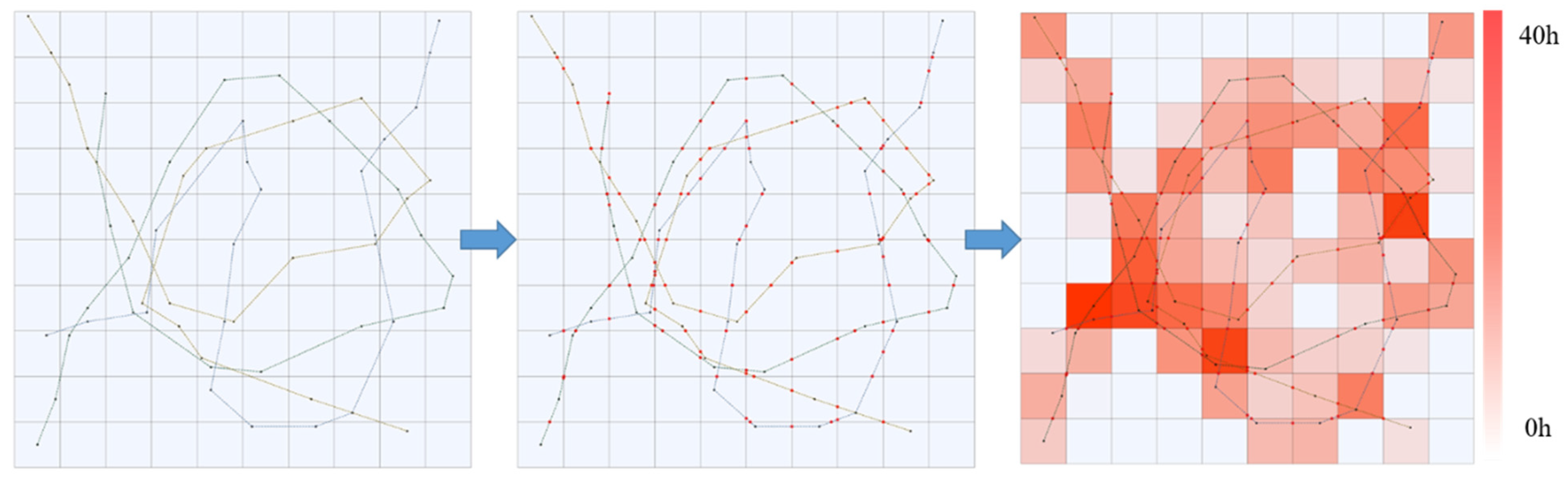
• Division of spatial grids: Divide the research sea area into a series of closely arranged spatial grids, with a spatial size of 5000 m × 5000 m for each grid set in this article;
• Grid based fishing trajectory segmentation: As shown in Figure 10, black dots represent the track points of the AIS fishing trajectory, and red dots represent the intersection point of the fishing trajectory and the spatial grid. By segmenting the fishing trajectory through the intersection point between the spatial grid and the fishing trajectory, a set of fishing trajectories for different fishing vessels within each spatial grid is obtained, denoted as $S_{grid}$.

  $$S_{grid}=\left\{T_{1,grid},\dots ,T_{n,grid},\dots ,T_{N,grid}\right\}$$

  (23)

In Equation (23) n represents different fishing vessels and $T_{m,grid}$ represents the corresponding fishing trajectory fragments within the spatial grid of fishing vessel n;

3.

Calculate fishing effort: calculate the total number of fishing attempts or fishing duration of all fishing trajectories in each spatial grid and evaluate the fishing intensity in each spatial grid. The calculation method is as follows:

$$F{E}_g={\displaystyle {\sum }_{i=1}^N{\displaystyle {\sum }_{j=0}^M{t}_{ij}}}$$

(24)

In Equation (24), $F{E}_g$ represents the fishing intensity of the grid, $t_{ij}$ represents the jth fishing duration of the fishing vessel i in the spatial grid, when $t_{ij}$ = 1, the final result is the statistics of the number of fishing. N represents the number of fishing vessels performing fishing operations in the grid, and M represents the number of fishing trajectory fragments of the fishing vessel i in the spatial grid.

4. Experiment and Result Analysis

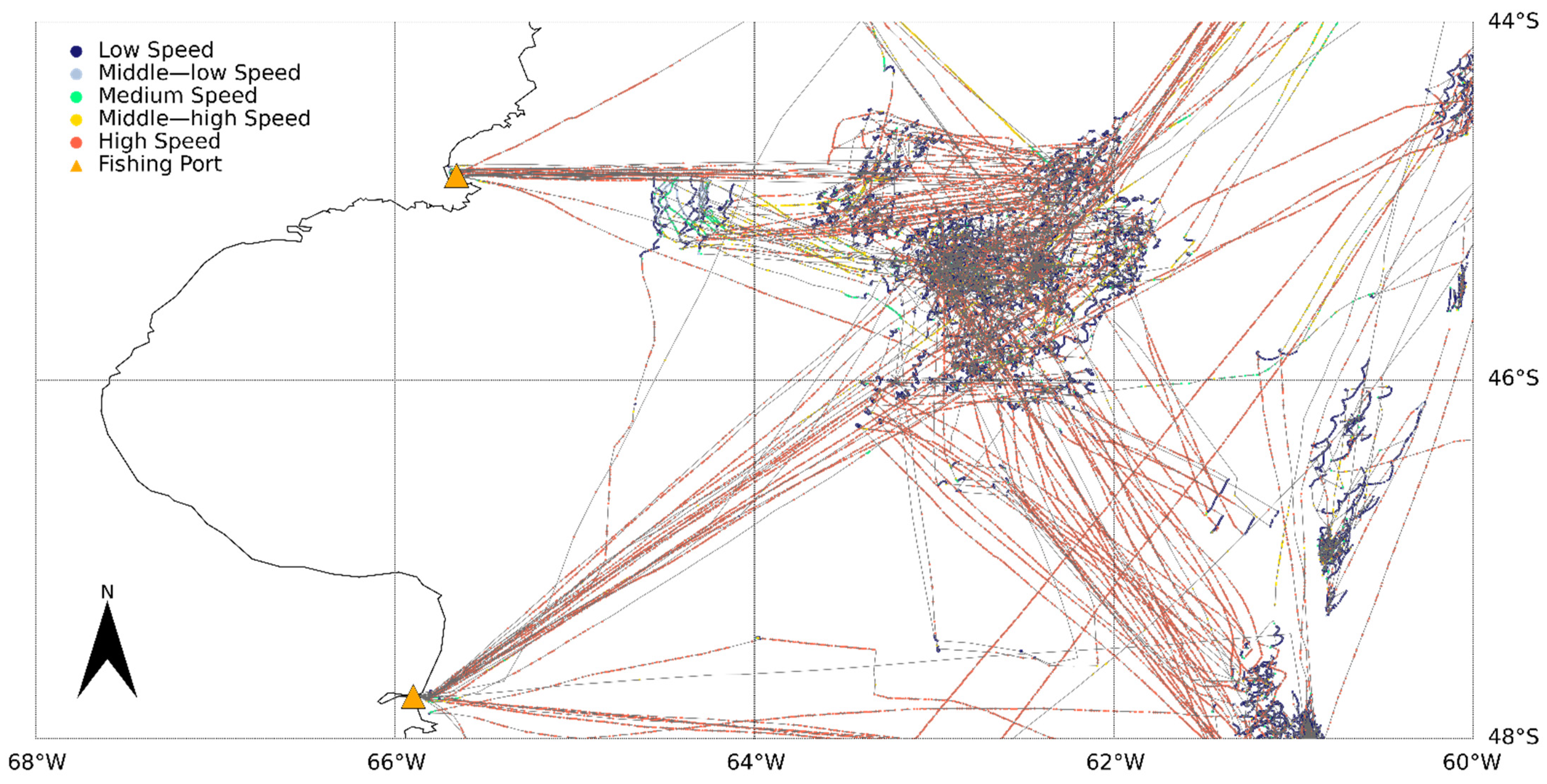
4.1. Experimental Area and Data

Since squid fishing vessel data is more abundant among the provided fishing vessel AIS data, all of the AIS data used in this study originated from Chinese squid fishing vessels that fished offshore in the Argentine seas in 2020. AIS data, fishing vessel logbooks, and vessel file lists are the main data sources for this study. We mainly write the code in python to implement the relevant algorithm.

A range of dynamic and static data is recorded in the AIS data of fishing vessels. MMSI, position coordinates, reporting time, speed, and course are all included in the dynamic information. MMSI, ship name, call sign, IMO, ship length (m), and ship breadth (m) are among the static information. The information in the fishing logbook comprises the name of the vessel, its type, its behavior status, the time the net or hook was set, its latitude and longitude, and the fish that were caught. Project name, project type, ship name, MMSI, and gear type are all included in vessel file lists. The suggested journey extraction approach is validated by comparing the worldwide port index data with the experimental findings. It is worth adding that the worldwide port index data cannot fully cover all port information in the world, which is why we proposed to identify fishing ports based on AIS data.

Table 1. Static and dynamic information of fishing vessel.

Data Type	Dynamic Data	Static Data	Note
AIS	Latitude, longitude, speed (knots), course (degree)	mmsi, ship name, call Sign, IMO, ship length (m), ship width (m)	The AIS data in this paper is parsed to include the reporting time (utc) information.
Fishing vessel logbook	Operation status, start time (utc), latitude of start point, longitude of start point, fish catch (Kg), reporting time (utc)	log_type, ship name	Operation status: fishing, nomal sailing.
Vessel file list	Null	project name, project type, ship name, mmsi, gear type	Project type: high seas project, transoceanic project.
World Port Index	Null	Index_no, Region_no, Port name, Country, Latitude, Longitude, Harbor size, etc.	With a wealth of geographical information and attributes of each port, this table does not enumerate too much.

displays the data utilized for the experiments in this paper and its format.

The AIS data of the fishing vessels did not show any indication of fishing operations. The fishing vessel log records the cast net time, denoted as utc_f. However, it has been discovered that the actual catch volume occasionally varies from the data in the logbook and that many fishing operations are not documented consistently, which is one of the main reasons why estimating the catch by the logbook can lead to an underestimation of the fishing effort.

Therefore, this article extracts the fishing trajectories and normal sailing trajectories of fishing vessels through visualization, combining fishing vessel logs and expert knowledge. The visualization results are shown in Figure 11. The velocity of the fishing vessel is divided into five intervals and displayed in five different colors in the image, thus intuitively representing the velocity changes and spatial structure of the ship’s trajectory. It is easy to see that a single voyage trajectory may involve one or more intensive fishing operations, and such areas are referred to as fishing areas. There are short-distance normal sailing routes and a range of fishing chances at the different fishing areas, which are connected by long-distance normal sailing routes.

In summary, as shown in Figure 12, this article extracts trajectory samples in two steps.

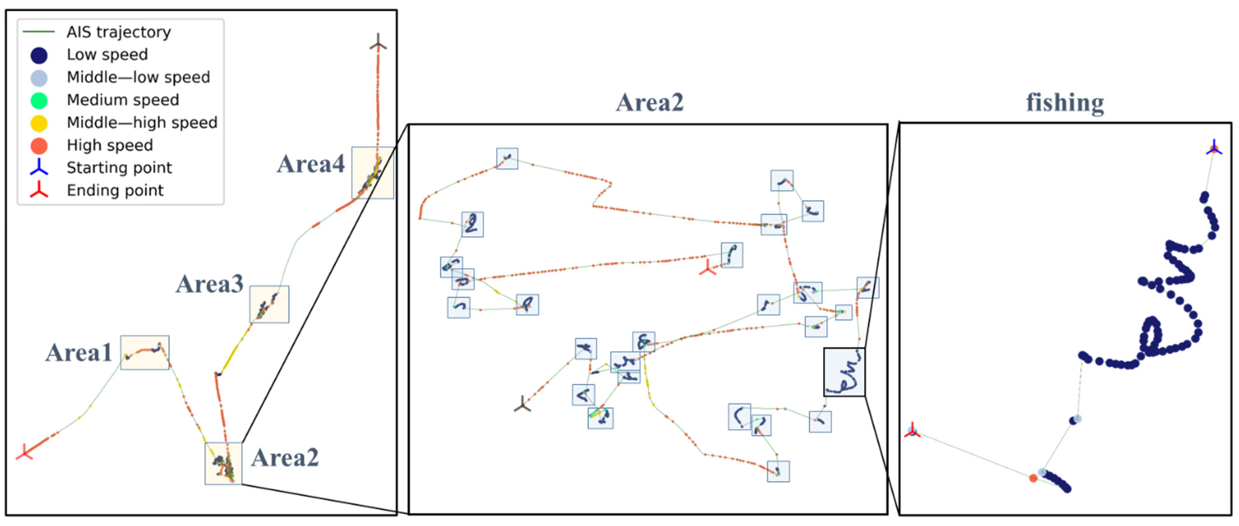
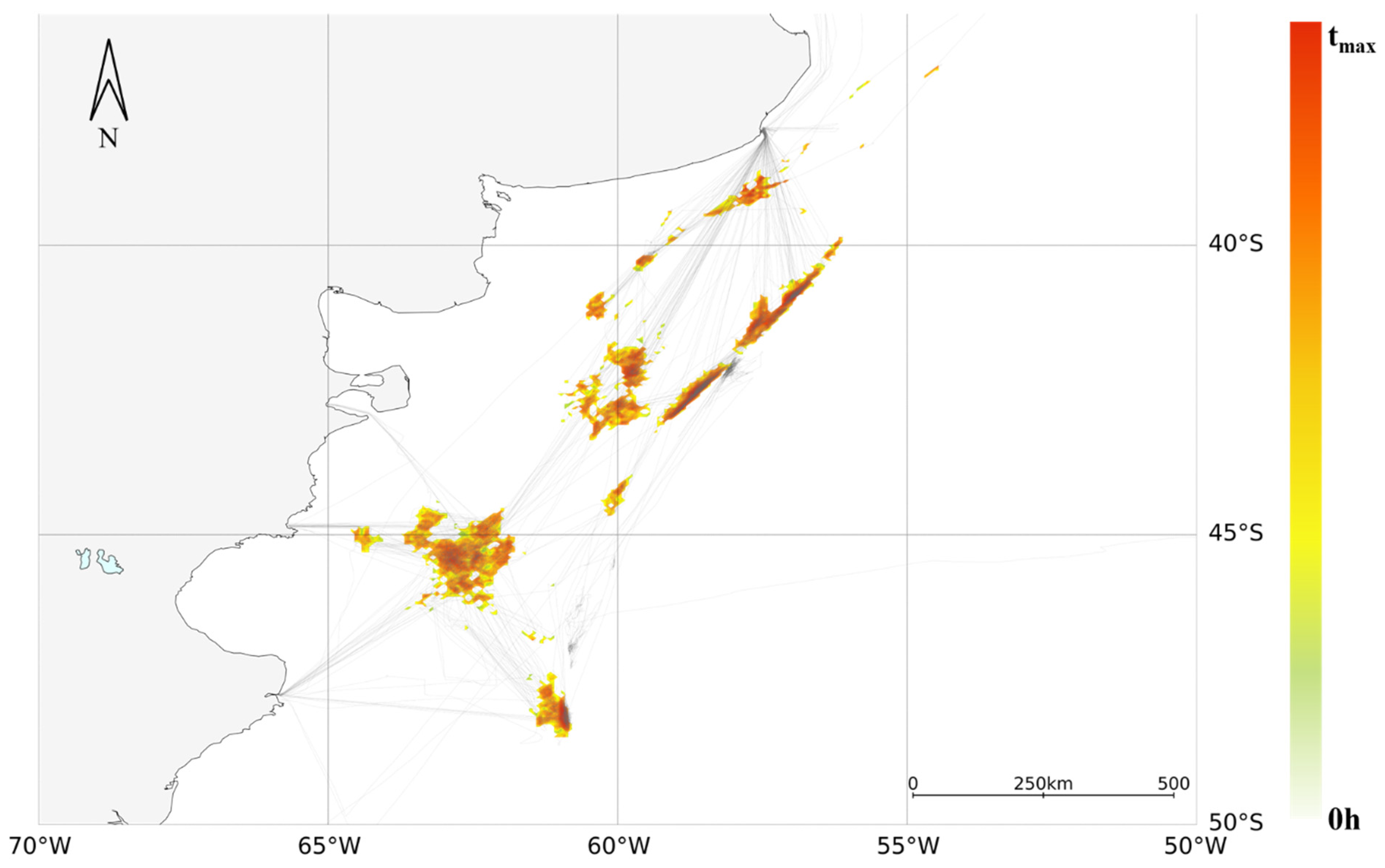
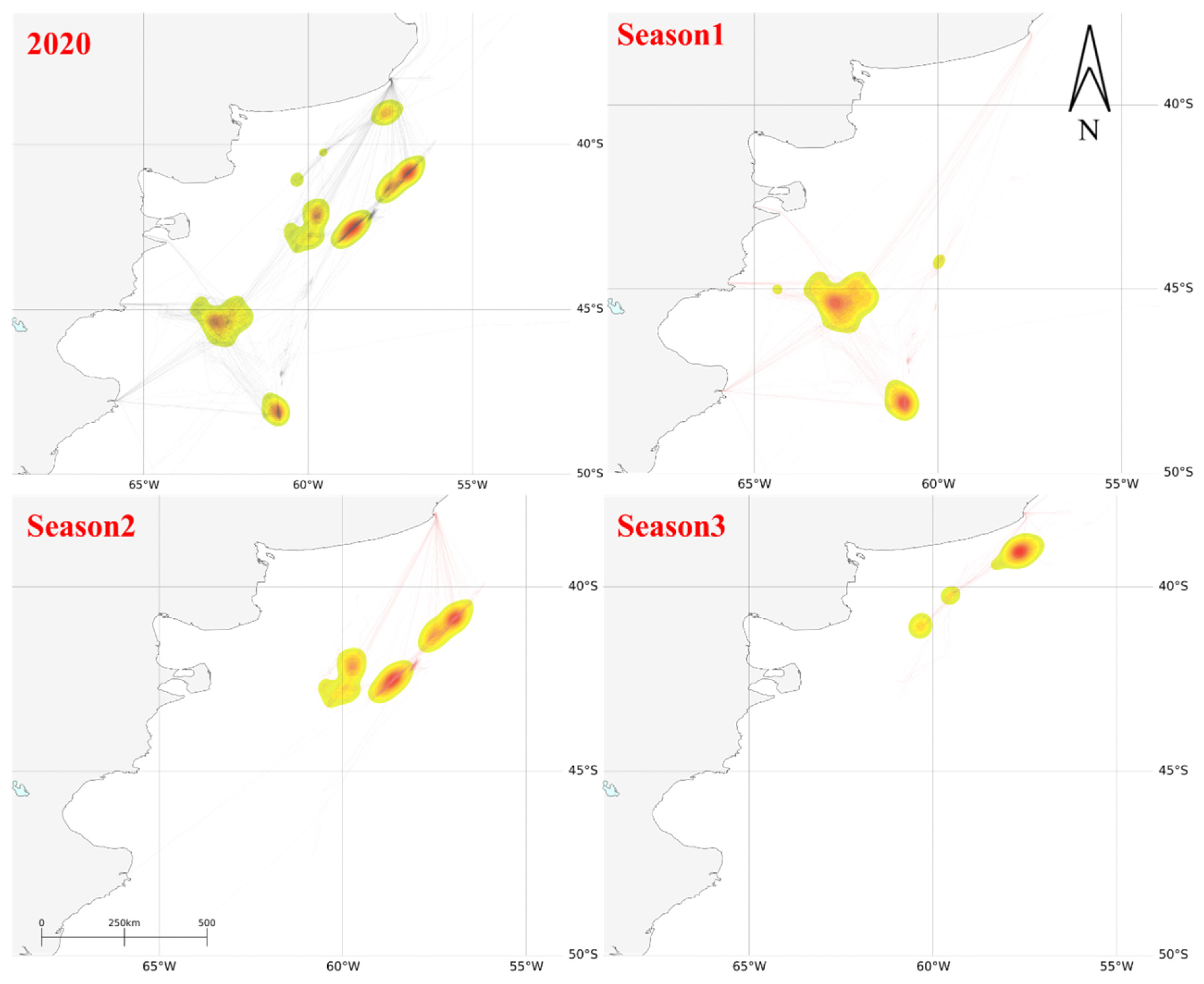
• Visualize the voyage trajectories of fishing vessels and extract the main fishing areas.
• Extracting fishing trajectory samples from fishing areas by combining the cast net time recorded in fishing vessel logs with expert knowledge.

This article randomly selected 120 voyage trajectories from AIS data and extracted 1000 fishing trajectories samples and 1000 normal sailing trajectories samples of squid fishing vessels, jointly composed of 2000 trajectory sample datasets.

As shown in Figure 13, the distribution probabilities of the duration and navigation mileage of 2000 trajectory samples were first calculated. Even though the duration of most fishing trajectory samples is longer than normal navigation trajectory samples, the navigation distance of normal navigation trajectory samples is much higher than fishing trajectory samples.

At the same time, we calculated six global statistical characteristics for all trajectory samples.

The global statistical characteristics of motion and morphology between fishing trajectory samples and normal sailing trajectory samples are presented, respectively.

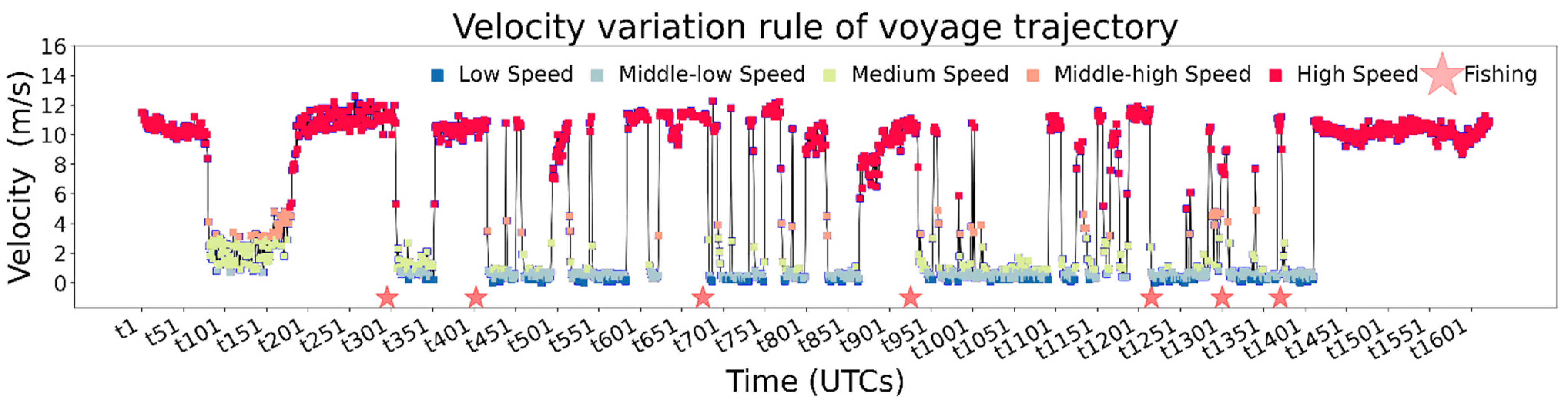
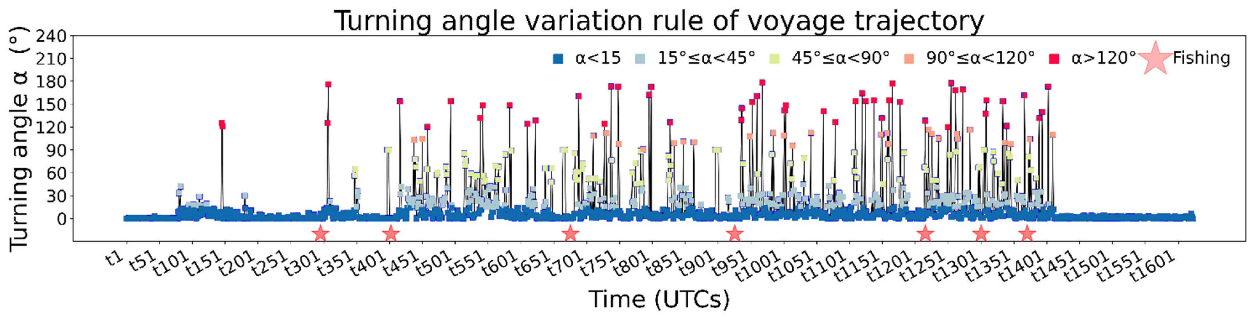
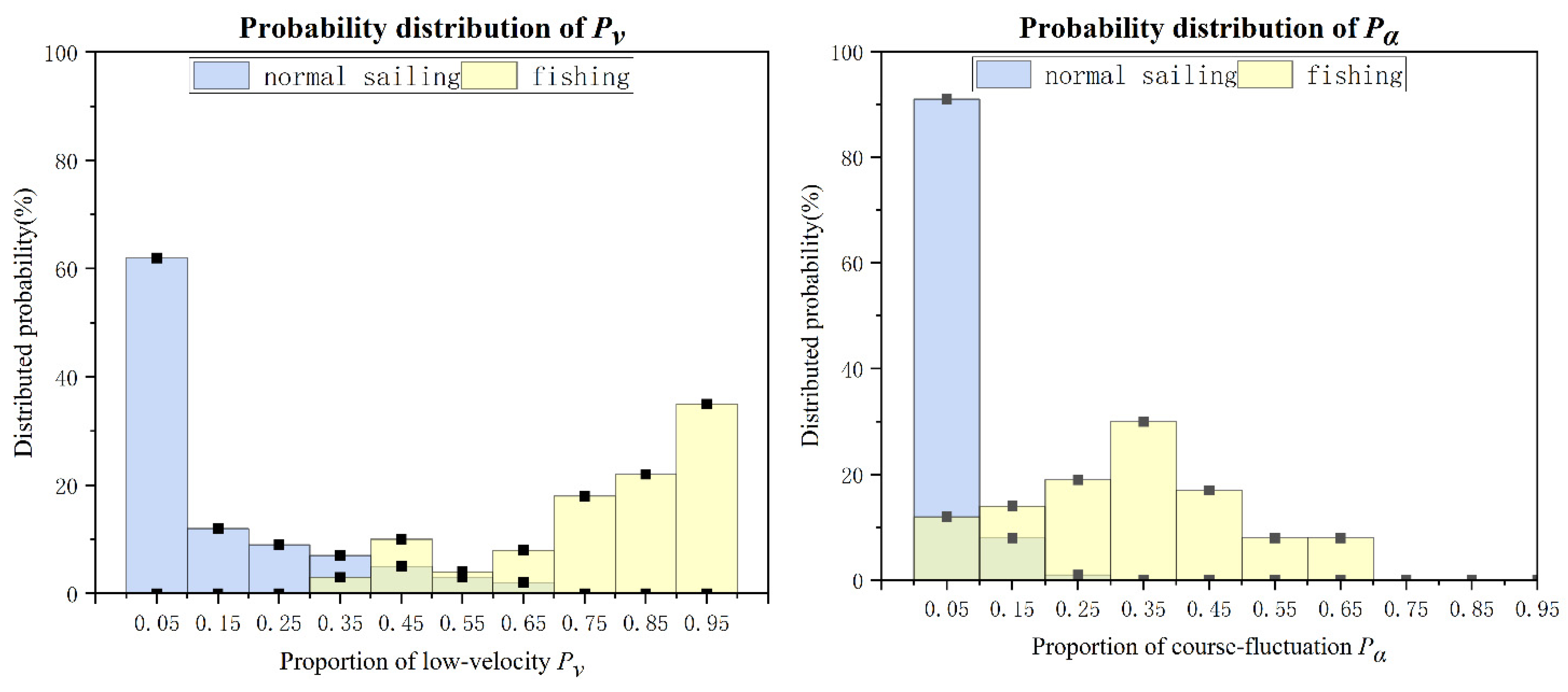
• As shown in Figure 14, the statistical results indicate that the fishing behavior of fishing vessels does maintain lower speeds and generate more frequent turns compared to normal sailing behavior. At the same time, it is explained that the $P_v$ and $P_{\alpha }$ defined from the perspective of motion can effectively distinguish between fishing trajectories and normal sailing trajectories.
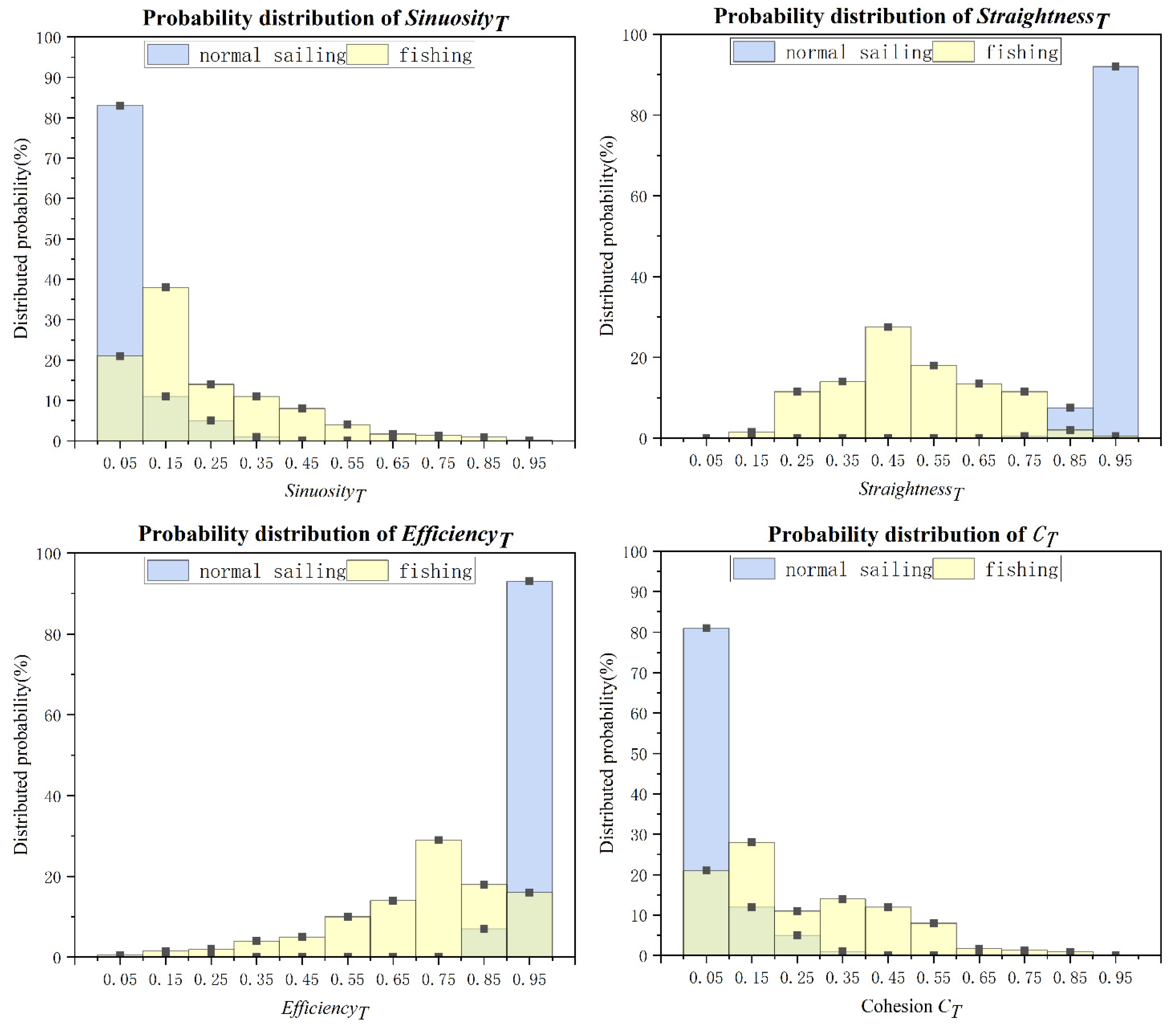
• As shown in Figure 15, the statistical results indicate that the four statistical characteristics $c_T$, $sinuosit{y}_T$, $straightnes{s}_T$, and $efficienc{y}_T$ defined from the perspective of trajectory morphology can also distinguish fishing trajectories from normal sailing trajectories from different aspects.

4.2. Method Evaluation

This article verifies the effectiveness of the proposed method for detecting the fishing behavior trajectory of squid fishing vessels from three aspects.

Voyage extraction verification: this article uses the voyage extraction method proposed in this article to identify the main fishing ports of squid fishing vessels in Argentine waters from AIS data and compares it with the port information in the global port index dataset to verify the effectiveness of this method.

The World Port Index, which is freely accessible from the National Geospatial-Intelligence Agency’s website (https://msi.nga.mil/Publications/WPI, accessed on 1 December 2021), is where the list of ports is compiled. The Global Port Index (Pub 150) is a table-based resource that lists the locations, physical qualities, amenities, and services provided by the world’s major ports and terminals (about 3700 entries).

Using data comparison, it can be determined that PUERTO MADRYN, LA PLATA, PUERTO DESEADO, and MAR DEL PLATA are the principal fishing ports where the target fishing vessels in this study dock. The name and locations information for the fishing ports, which are scattered over Argentina’s east coast, and were identified from AIS data are shown in

Table 2. Coordinates of the center point of anchorages.

Port Name	LON	LAT
MAR DEL PLATA	−57.516008	−38.022194
LA PLATA	−57.890093	−34.822192
PUERTO DESEADO	−65.898126	−47.765125
PUERTO MADRYN	−65.027862	−42.738157
Not Matched	−65.658333	−44.860000

.

As seen in Figure 16, the blue dot represents the ports recorded in the World Port Index, and the red circle represents the stopping fishing ports identified from the AIS data. By comparing and analyzing the results of fishing vessels with the ports recorded in the World Port Index, four fishing ports identified from AIS data matched the corresponding ports recorded in the Global Port Index. A fishing port identified from AIS data is located at 44.86° W and 65.66° S, but it is not recorded in the World Port Index. It proved that the voyage extraction method proposed in this article can still identify every fishing port in the absence of port data.

Points of Interest Verification: This paper verifies the correlation between the transition from normal sailing to fishing operation status of squid fishing vessels and the occurrence of speed decreases by combining the AIS trajectory with the fishing start moment recorded in the fishing vessel logbook. The specific implementation methods are:

• If the fishing logbook records the fishing start moment as utc_f, set the time interval as [utc_f − t_ε, utc_f + t_ε].
• Extract the AIS trajectory of the fishing vessel in this time interval.
• Judge whether the trajectory has experienced a change in speed interval (from a high-speed portion to a low-speed section).
• Calculate the proportion of the fishing log records that satisfy the condition to the total number of fishing log reports, P_poi.

Table 3. The changes of P_poi corresponding to different time intervals t_ε.

tε	Ppoi
0.1 h	66.3%
0.2 h	81.8%
0.5 h	88.4%
1 h	97.5%
1.5 h	100%
2 h	100%

shows that although the starting point of the fishing trajectory of fishing vessels cannot be accurately judged by speed drop, it still proves that there is a strong correlation between the transition from normal sailing to fishing operation state and speed drop.

Fishing behavior detection model verification: the confusion matrix is typically produced for the binary model test, and fishing behavior is used as a positive example. The following calculation formulas are used to evaluate the recognition model according to its calculation accuracy, precision, recall rate, and specificity.

$$Accuracy=\frac{TP+TN}{TP+TN+FP+FN}$$

(25)

$$Precision=\frac{TP}{TP+FP}$$

(26)

$$Recall=\frac{TP}{TP+FN}$$

(27)

$$Specificity=\frac{TN}{TN+FP}$$

(28)

In Equations (25)–(28), $TP$ stands for the number of fishing behaviors that were correctly identified, $FP$ for those that were wrongly identified, $TN$ for the number of normal sailing behaviors that were correctly identified, and $FN$ for those that were incorrectly identified.

The F1-Score and Kappa coefficient were generated to assess the model’s resilience and classification accuracy, respectively, in order to fully validate the model’s validity. The following are the calculating Equations (29)–(31):

$$pe=\frac{(TP+FN)\times (TP+FP)+(FP+TN)\times (FN+TN)}{N^2}$$

(29)

$$Kappa=\frac{A-pe}{1-pe}$$

(30)

$$F1=\frac{2TP}{2TP+FN+TN}$$

(31)

In order to compare the effectiveness of the fishing behavior trajectory detection model proposed in this article with the point-by-point fishing behavior detection model, two experiments were conducted separately.

• In experiment 1, 75% of the data sets were used to test the logistic regression model, and 25% of the data sets were randomly chosen to train the model’s parameters.
• In experiment 2, a point-by-point detection model based on speed threshold was adopted. The sample object was transformed into track points, so 2000 trajectory datasets were further decomposed to obtain 194,356 fishing track point samples and 177,364 normal sailing track points. This article randomly selects 5000 fishing track point samples and 5000 normal sailing track point samples as the test dataset for Experiment 2 and set the speed threshold at 4 m/s.

Table 4. Confusion table of the testing dataset.

Experiments	Real Type Label	Predict Classification Results
		Fishing	Normal Sailing
Experiment 1	Fishing	4036	964
	Normal sailing	1153	3847
Experiment 2	Fishing	1484	16
	Normal sailing	8	1492

displays the confusion matrix of two experiments, sometimes called an error matrix. Calculate the relevant evaluation indicators based on the experimental results in Table 2. The relevant evaluation indicators for the two experiments are as follows:

(1)

The accuracy of the test data set in Experiment 1 was 78.83%, the precision was 80.72%, the recall rate was 77.78%, the specificity was 79.96%, the Kappa coefficient was 0.5766, and the f1-Score was 0.7922.

(2)

The accuracy of the test data set in Experiment 2 was 99.20%, the precision was 98.93%, the recall rate was 99.46%, the specificity was 98.94%, the Kappa coefficient was 0.9840, and the f1-Score was 0.9920.

4.3. Results Analysis

This article takes the AIS data of 12 squid fishing vessels in Argentine waters as an example to calculate and discuss the overall and individual fishing activities of squid fishing vessels. (1) The spatial distribution and variation patterns of annual and quarterly fishing activities, AND (2) A detailed evaluation of individual fishing activities.

The spatial distribution of the annual fishing activities of 12 fishing vessels is shown in Figure 17. The 12 fishing vessels spent 48,503 h at sea in 2020, of which 16,596 h were used for fishing operations, and 919 fishing activities were carried out throughout the year, with an average length of about 17.5 h. This information was obtained through statistical analysis of the experimental results. The 12 fishing boats covered 236,067 km during the fishing trip. The fishing operation covered 46,836 km. Figure 11 displays the results of the calculation in graphic form. In 2020, we will be able to know where the most popular fishing spots are located.

The spatial distribution of fishing activities in the three quarters of January–March, April–June, and July–September can be determined based on the seasonal division of the yearly fishing behavior trajectory. As illustrated in Figure 18, it is possible to further investigate how fishing activity’s geographical distribution changes with the seasons. It was discovered that during January and March, Chinese squid fishing vessels operating in the Argentinean Sea were mostly positioned in two zones of active fishing, each with a space range of 46.2° to 44.5° S and 61.5° to 63.8° W. A significant trend in worldwide marine fisheries governance is the promotion of sustainable fisheries development. Achieving sustainable fisheries, illegal fishing regulations, compliance and enforcement of monitoring, control, and surveillance measures, fishing overcapacity, extensive use of pelagic drift nets, sub-regional and regional cooperation, bycatch, and discards, among other things, are the top seven issues [29]. Marine fisheries governance now primarily focuses on illegal fishing practices among these [30].

The monitoring of fishing vessel activities at sea cannot be narrowed down to specific fishing vessels because of the limited traceability of the overall evaluation approach to the footprint of those activities in prior studies. The detection method based on track segments can precisely meet this demand because, in the modern world, we are not only concerned with the overall spatial and temporal distribution of fishing vessel activities but also with the changes in fishing activities of each fishing vessel throughout the year. Given that the detection outcome based on the track segment is a full fishing track segment, it is able to further extrapolate the spatial and temporal information of each fishing operation and perform a quantitative analysis of the annual fishing frequency and the annual mileage and time of fishing activities of each fishing vessel.

Table 5. Single-vessel fishing information statistics.

MMSI	Number of Sea Trips	Total Mileage Sailed	Total Fishing Mileage	Number of Fishing Trips	Total Sailing Time	Total Fishing Time
701 ** 3000	10	16,994	3990	51	3588	1544
701 ** 6788	18	20,296	3599	49	4294	1248
701 ** 6615	7	16,688	5219	60	3761	1851
701 ** 6609	7	13,928	1279	57	3246	450
701 ** 6614	15	16,905	5757	110	4197	2141
701 ** 6000	12	18,759	5366	140	3814	1887
701 ** 4000	8	15,908	4179	41	3036	1347
701 ** 6568	10	15,928	4591	98	3817	1390
701 ** 0674	6	10,150	3564	176	2405	996
701 ** 5000	11	17,373	5231	65	3714	1954
701 ** 6725	14	18,004	4057	72	3842	1783
412 ** 0688	1	55,127	0	0	8783	0

MMSI is hidden with the * symbol.

displays the various indicators for various vessels after statistical calculation, including six statistical indicators, such as the number of sea trips, total distance traveled, total distance traveled for fishing, number of fishing trips, total sailing time, and total distance traveled for fishing. At the same time, more information can be gleaned from the chart’s data by further mining it. One indicator that may be used to gauge the effectiveness and intensity of fishing trips is the ratio between the indicators for “number of fishing trips” and “number of sea trips,” which shows the typical number of fishing trips completed by fishing vessels. The average total fishing time and single fishing tie time of fishing vessels can be determined using the number of sea trips, total fishing time, and total sailing time indicators. These metrics, which to some extent reflect the work intensity of fishing vessel crews at sea and provide a data foundation for how to protect the legal rights of crews, can be used to calculate the average total fishing time and single fishing tie time of fishing vessels.

Table 6. Quantitative analysis of the monthly fishing frequency of different squid fishing vessels.

MMSI	January	February	March	April	May	June	July	August	September	October	November	December
701 ** 3000	10	8	10	6	6	7	4	0	0	0	0	0
701 ** 6788	7	1	1	8	13	8	10	1	0	0	0	0
701 ** 6615	9	7	8	9	18	6	3	0	0	0	0	0
701 ** 6609	9	2	0	46	0	0	0	0	0	0	0	0
701 ** 6614	26	36	6	6	11	7	17	1	0	0	0	0
701 ** 6000	14	18	18	22	45	16	7	0	0	0	0	0
701 ** 4000	9	10	8	4	9	1	0	0	0	0	0	0
701 ** 6568	7	6	4	20	41	11	2	0	0	0	0	0
701 ** 0674	39	52	60	0	11	0	0	0	0	0	0	0
701 ** 5000	13	7	9	6	16	6	6	0	0	0	0	0
701 ** 6725	4	6	5	15	13	9	13	7	0	0	0	0
412 ** 0688	0	0	0	0	0	0	0	0	0	0	0	0

MMSI is hidden with the * symbol.

shows how the patterns of fishing frequency change with the months for different fishing vessels. The table makes it clear that fishing activities by fishing vessels only took place from January to September and that the overall trend remained stable, displaying a general decline month by month. After August, we anticipate a four-month fishing moratorium for all local squid fishing boats. The majority of fishing vessels’ busiest months for fishing are February and May. The daily change in the number of fishing vessels can be further adjusted, if necessary, from the monthly variation. By doing so, we can assess the fishing activities of fishing vessels throughout the course of the entire year and examine variations in those activities over time, which forms the basis for ongoing monitoring and oversight of fisheries.

The model and method suggested in this study can accurately determine the ports from which fishing vessels depart and return for each fishing trip, and the geographic scope and timing of each fishing operation. Thus, the relevant departments can use the precise data findings to determine whether the fishing vessels have engaged in illegal behavior, we can further refine the data supervision of each fishing vessel for each fishing trip.

The statistics pertaining to each of the single voyage sub-trajectories undertaken by one of the fishing vessels used as an example in this paper are displayed in the

Table 7. Voyage trajectories’ information statistics.

Voyages	Departing Port	Arriving Port	Departing Time	Arriving Time	Number of Fishing Trips
Track1	LA PLATA	MAR DEL PLATA	2020-01-08 19:37:21	2020-01-09 16:21:32	0
Track2	MAR DEL PLATA	MAR DEL PLATA	2020-01-09 18:00:51	2020-01-14 21:30:36	1
Track3	Not Matched	MAR DEL PLATA	2020-01-16 05:09:23	2020-02-10 03:22:56	11
Track4	MAR DEL PLATA	MAR DEL PLATA	2020-02-13 12:46:26	2020-03-26 04:28:17	14
Track5	PUERTO DESEADO	MAR DEL PLATA	2020-03-28 23:59:51	2020-04-16 01:38:58	6
Track6	MAR DEL PLATA	MAR DEL PLATA	2020-04-21 01:14:56	2020-04-29 02:29:29	2
Track7	MAR DEL PLATA	MAR DEL PLATA	2020-04-30 10:04:37	2020-05-19 22:45:36	6
Track8	MAR DEL PLATA	MAR DEL PLATA	2020-06-05 05:33:07	2020-07-04 16:46:26	10
Track9	MAR DEL PLATA	MAR DEL PLATA	2020-07-04 18:11:47	2020-07-05 14:56:48	1
Track10	MAR DEL PLATA	MAR DEL PLATA	2020-07-30 22:20:01	2020-07-31 21:02:03	0

. The information in the table tells us that MAR DEL PLATA is the fishing port where the vessel returns after its fishing expedition; however, there are other ports that can be used as departure points. The Global Port Index list of ports does not include the ship’s departure port for its third fishing expedition in 2020. Intriguingly, we discovered that on 16 January 2020, at around 5:00 a.m., all the fishing vessels in the research left this fishing port.

Using the fishing detection method for squid proposed in this paper, we can further obtain the space-time information of each fishing activity. Taking one of the single voyage sub-trajectories (Track 8) of fishing vessels as an example, the information of each fishing trajectories is shown in the

Table 8. Fishing trajectories’ information statistics.

Voyages	Fishing Trajectories	Lon_Start	Lat_Start	Start Time	Stop Time
Track 8	Fishing1	−64.235245	−44.869124	2020-06-11 23:37:05	2020-06-12 06:02:54
Track 8	Fishing2	−63.612587	−44.987512	2020-06-14 21:08:31	2020-06-15 05:40:16
Track 8	Fishing3	−63.605215	−45.003654	2020-06-15 22:09:35	2020-06-16 07:12:07
Track 8	Fishing4	−62.358074	−44.654007	2020-06-18 23:24:58	2020-06-19 06:45:51
Track 8	Fishing5	−62.312457	−45.215800	2020-06-21 23:55:04	2020-06-22 09:00:54
Track 8	Fishing6	−62.680040	−44.760542	2020-06-24 00:23:12	2020-06-24 07:14:06
Track 8	Fishing7	−62.002415	−45.752023	2020-06-24 22:42:27	2020-06-25 04:59:42
Track 8	Fishing8	−62.841567	−45.741200	2020-06-25 23:37:11	2020-06-26 08:04:31
Track 8	Fishing9	−63.001400	−45.023350	2020-06-27 20:57:08	2020-06-28 08:10:44
Track 8	Fishing10	−64.254100	−45.214740	2020-06-29 22:45:34	2020-06-30 06:56:21

:

In this single voyage sub-trajectory, the fishing activities are mainly concentrated from 11 June to 29 June, and the spatiotemporal information of each fishing activity is completely recorded. In addition to completing the whole activity evaluation of fishing vessels by AIS, as demonstrated above, the model and approach suggested in this work may also enhance the traceability of fishing vessel operations and enable high-precision fishing vessel monitoring.

The evaluation at various scales shows that the strategy put forth in this study can be used in a wide range of scenarios when dealing with difficult fisheries management requirements. It provides a powerful supporting force for monitoring, controlling, and surveillance of fishing vessels because it not only assesses the spatial distribution of fishing activities of fishing vessels from a macroscopic perspective but also captures the precise spatiotemporal information of each fishing trip of fishing vessels.

5. Conclusions

In this study, numerous global statistical aspects of the trajectory segment were established using the AIS data and fishing logs of Chinese squid fishing vessels in the Argentine Sea area as research objects. A methodology for detecting the fishing behavior of squid fishing vessels was developed based on the logistic regression model. Global statistical features from motion and form views have been added, and the sliding window has been optimized. As a result, its accuracy has increased to 99.20%, and its overall evaluation index is favorable. Comparing the trajectory segment to the detection model with track points as the minimal expression unit, the trajectory segment may more accurately and extensively portray the fishing behavior of fishing vessels. By focusing on different studies’ research topics, we may comprehend the annual average macroscopic intensity of squid fishing activity, the characteristics of its spatial distribution, and the phenomena of its spatial migration with changes in fishing grounds every three months. We can simultaneously track detailed information about every fishing vessel, every journey trajectory, and even every fishing action.

In the analysis part, this paper describes the analysis of the results of squid fishing trajectories in detail. Unlike the point-by-point fishing detection model, the method proposed in this paper can extract the start time, end time, and complete fishing trajectory of each independent fishing behavior. This method improves the transparency and traceability of the fishing behavior of fishing vessels and provides strong data support for fishing regulation. In future research, other data sources can be introduced, such as geographical boundary information of marine environmental protection areas, management rules of closed fishing seasons, etc., to complete the detection and attack of illegal fishing.

The goal of the study and its scope are illustrated by squid fishing boats operating in the Argentinean maritime region, but they can be applied to other geographic areas and even to additional fishing boats engaged in different types of fishing operations. The long-term development of the world’s pelagic fisheries will receive more thorough technical support if different types of fishing vessels’ fishing activity can be detected.

References

1. Lira, A.S.; Lucena-Frédou, F.; Lacerda, C.H.F.; Eduardo, L.N.; Ferreira, V.; Frédou, T.; Ménard, F.; Angelini, R.; Le Loc'h, F. Effect of fishing effort on the trophic functioning of tropical estuaries in Brazil. Estuar. Coast. Shelf Sci. 2022, 277, 108040. [Google Scholar] [CrossRef]
2. Schartup, A.T.; Thackray, C.P.; Qureshi, A.; Dassuncao, C.; Gillespie, K.; Hanke, A.; Sunderland, E.M. Climate change and overfishing increase neurotoxicant in marine predators. Nature 2019, 572, 648–650. [Google Scholar] [CrossRef] [PubMed]
3. Agnew, D.J.; Pearce, J.; Pramod, G.; Peatman, T.; Watson, R.; Beddington, J.R.; Pitcher, T.J. Estimating the worldwide extent of illegal fishing. PLoS ONE 2009, 4, e4570. [Google Scholar] [CrossRef] [PubMed] [Green Version]
4. Syversen, T.; Lilleng, G.; Vollstad, J.; Hanssen, B.J.; Sonvisen, S.A. Oceanic plastic pollution caused by Danish seine fishing in Norway. Mar. Pollut. Bull. 2022, 179, 113711. [Google Scholar] [CrossRef]
5. Vince, J.; Hardesty, B.D.; Wilcox, C. Progress and challenges in eliminating illegal fishing. Fish. Res. 2021, 22, 518–531. [Google Scholar] [CrossRef]
6. Fabinyi, M.J.G. Maritime disputes and seafood regimes: A broader perspective on fishing and the Philippines–China relationship. Globalizations 2020, 17, 146–160. [Google Scholar] [CrossRef]
7. Shih, Y.-C.; Chang, Y.-C.; Gullett, W.; Chiau, W.-Y. Challenges and opportunities for fishery rights negotiations in disputed waters–A Taiwanese perspective regarding a fishing boat case incident. Mar. Policy 2020, 121, 103755. [Google Scholar] [CrossRef]
8. Mangi, S.C.; Kenny, A.; Readdy, L.; Posen, P.; Ribeiro-Santos, A.; Neat, F.C.; Burns, F. The economic implications of changing regulations for deep sea fishing under the European Common Fisheries Policy: UK case study. Sci. Total Environ. 2016, 562, 260–269. [Google Scholar] [CrossRef] [PubMed]
9. Wu, H.; Li, Q.; Wang, C.; Wu, Q.; Peng, C.; Jefferson, T.A.; Long, Z.; Luo, F.; Xu, Y.; Huang, S.-L. Bycatch mitigation requires livelihood solutions, not just fishing bans: A case study of the trammel-net fishery in the northern Beibu Gulf, China. Mar. Policy 2022, 139, 105018. [Google Scholar] [CrossRef]
10. Ji, J.; Li, Y. The development of China's fishery informatization and its impact on fishery economic efficiency. Mar. Policy 2021, 133, 104711. [Google Scholar] [CrossRef]
11. Zhou, S.; Smith, A.D.; Knudsen, E.E. Ending overfishing while catching more fish. Fish Fish. 2015, 16, 716–722. [Google Scholar] [CrossRef]
12. Solarin, S.A.; Gil-Alana, L.A.; Lafuente, C. Persistence and sustainability of fishing grounds footprint: Evidence from 89 countries. Sci. Total Environ. 2021, 751, 141594. [Google Scholar] [CrossRef]
13. Feng, B.; Li, Z.; Lu, H.; Yan, Y.; Hou, G. Estimating the total allowable catch and management of Threadfin porgy (Evynnis cardinalis) fisheries in the northern South China Sea based on sampling surveys conducted at fishing ports. Aquaculture 2022. Advance online publication. [Google Scholar] [CrossRef]
14. Venerus, L.A.; Parma, A.M. An access-point survey approach to estimate recreational boat-fishing effort for stays of variable length. Fish. Res. 2022, 254, 106429. [Google Scholar] [CrossRef]
15. Constantino, M.M.; Cubas, A.L.V.; Silvy, G.; Magogada, F.; Moecke, E.H.S. Impacts of illegal fishing in the inland waters of the State of Santa Catarina–Brazil. Mar. Pollut. Bull. 2022, 180, 113746. [Google Scholar] [CrossRef]
16. Quimbayo, J.P.; Silva, F.C.; Barreto, C.R.; Pavone, C.B.; Lefcheck, J.S.; Leite, K.; Figueiroa, A.C.; Correia, E.C.; Flores, A.A.V. The COVID-19 pandemic has altered illegal fishing activities inside and outside a marine protected area. Curr. Biol. 2022, 32, R765–R766. [Google Scholar] [CrossRef] [PubMed]
17. Ribeiro, C.V.; Paes, A.; de Oliveira, D. AIS-based maritime anomaly traffic detection: A review. Expert Syst. Appl. 2023. Advance online publication. [Google Scholar] [CrossRef]
18. Yuan, Z.; Yang, D.; Fan, W.; Zhang, M. On fishing grounds distribution of tuna longline based on satellite automatic identification system in the Western and Central Pacific. Mar. Fish. 2018, 40, 649–659. [Google Scholar]
19. Yan, Z.; He, R.; Ruan, X.; Yang, H. Footprints of fishing vessels in Chinese waters based on automatic identification system data. J. Sea Res. 2022, 187, 102255. [Google Scholar] [CrossRef]
20. Ferrà, C.; Tassetti, A.N.; Grati, F.; Pellini, G.; Polidori, P.; Scarcella, G.; Fabi, G. Mapping change in bottom trawling activity in the Mediterranean Sea through AIS data. Mar. Policy 2018, 94, 275–281. [Google Scholar] [CrossRef]
21. Natale, F.; Gibin, M.; Alessandrini, A.; Vespe, M.; Paulrud, A. Mapping fishing effort through AIS data. PLoS ONE 2015, 10, e0130746. [Google Scholar] [CrossRef] [Green Version]
22. Kroodsma, D.A.; Mayorga, J.; Hochberg, T.; Miller, N.A.; Boerder, K.; Ferretti, F.; Wilson, A.; Bergman, B.; White, T.D.; Block, B.A. Tracking the global footprint of fisheries. Science 2018, 359, 904–908. [Google Scholar] [CrossRef] [Green Version]
23. Masroeri, A.; Aisjah, A.S.; Jamali, M.M. IUU fishing and transhipment identification with the miss of AIS data using Neural Networks. In Proceedings of the IOP Conference Series: Materials Science and Engineering, Sanya, China, 12–14 November 2021; p. 012054. [Google Scholar]
24. Zhang, C.; Chen, Y.; Xu, B.; Xue, Y.; Ren, Y. The dynamics of the fishing fleet in China Seas: A glimpse through AIS monitoring. Sci. Total Environ. 2022, 819, 153150. [Google Scholar] [CrossRef] [PubMed]
25. Yang, S.-l.; Zhang, S.-m.; Zhang, H.; Fei, Y.-j.; Jin, W.-g.; Wang, G.-l.; Fan, W. Pelagic fishing vessel classification using Bidirectional long short-term memory networks. Mar. Sci. 2022, 46, 25–35. (In Chinese) [Google Scholar] [CrossRef]
26. Zhang, L.; Lu, W.; Wen, J.; Cui, J. A detection and restoration approach for vessel trajectory anomalies based on AIS. J. Northwestern Polytech. Univ. 2021, 39, 119–125. (In Chinese) [Google Scholar] [CrossRef]
27. Liu, C.; Liu, J.; Zhou, X.; Zhao, Z.; Wan, C.; Liu, Z. AIS data-driven approach to estimate navigable capacity of busy waterways focusing on ships entering and leaving port. Ocean Eng. 2020, 218, 108215. [Google Scholar] [CrossRef]
28. Vermard, Y.; Rivot, E.; Mahévas, S.; Marchal, P.; Gascuel, D. Identifying fishing trip behaviour and estimating fishing effort from VMS data using Bayesian Hidden Markov Models. Ecol. Model. 2010, 221, 1757–1769. [Google Scholar] [CrossRef] [Green Version]
29. Fajardo, T. To criminalise or not to criminalise IUU fishing: The EU’s choice. Mar. Policy 2022, 144, 105212. [Google Scholar] [CrossRef]
30. Zhu, X.; Tang, J. The interplay between soft law and hard law and its implications for global marine fisheries governance: A case study of IUU fishing. Aquac. Fish. 2023; Advance online publication. [Google Scholar] [CrossRef]
Figure 1. Turning angle α i and direction error angle β i .
Jmse 11 01245 g001
Figure 2. Centerline distance h i and center distance d c , i .
Jmse 11 01245 g002
Figure 3. Velocity variation rule of voyage trajectory.
Jmse 11 01245 g003
Figure 4. Turning angle variation rule of voyage trajectory.
Jmse 11 01245 g004
Figure 5. Morphological characteristics of fishing trajectory.
Jmse 11 01245 g005
Figure 6. Workflow of fishing behavior detection.
Jmse 11 01245 g006
Figure 7. Diagram of voyage division.
Jmse 11 01245 g007
Figure 8. Squid fishing vessel speed distribution probability diagram.
Jmse 11 01245 g008
Figure 9. Points of interest diagram.
Jmse 11 01245 g009
Figure 10. Variable length sliding window diagram.
Jmse 11 01245 g010
Figure 11. Diagram of fishing effort calculation. Different colored tracks correspond to different fishing activities.
Jmse 11 01245 g011
Figure 12. Extraction steps of fishing trajectories samples.
Jmse 11 01245 g012
Figure 13. Distribution pattern of track duration and navigation mileage.
Jmse 11 01245 g013
Figure 14. Distribution pattern of trajectories characteristics based on motion.
Jmse 11 01245 g014
Figure 15. Distribution pattern of trajectories characteristics based on morphology.
Jmse 11 01245 g015
Figure 16. Visualization of fishing port results.
Jmse 11 01245 g016
Figure 17. Thermal map of annual grid fishing activities of squid fishing vessels.
Jmse 11 01245 g017
Figure 18. Seasonal spatial change of squid fishing vessels.
Jmse 11 01245 g018