Article

An Offshore Self-Stabilized System Based on Motion Prediction and Compensation Control

1
Lijiang Water Network Company, Yunnan Infrastructure Investment Co., Ltd., Lijiang 650500, China
2
School of Electrical & Information Engineering, Wuhan Institute of Technology, Wuhan 430205, China
3
Institute of Ocean Information Technology, Shandong Jiaotong University, Weihai 264200, China
4
School of Navigation, Wuhan University of Technology, Wuhan 430063, China
*
Authors to whom correspondence should be addressed.
J. Mar. Sci. Eng. 2023, 11(4), 745; https://doi.org/10.3390/jmse11040745
Submission received: 28 February 2023 / Revised: 20 March 2023 / Accepted: 28 March 2023 / Published: 29 March 2023

Abstract

:
The swaying motion of ships can always be generated due to the influence of complex sea conditions. A novel offshore Self-Stabilized system based on motion prediction and compensation control was studied. Firstly, an autoregressive model of ship motion exposed to various sea conditions was established, and the parameters of the model were initialized and updated by offline and online learning historical data. Using the autoregressive model with the acquired parameters, the prediction of the ship’s motion was achieved. Then, a Self-Stabilized system platform composed of six electric cylinders in parallel was designed, and the corresponding inverse kinematics were established. The corresponding controller using the result of motion prediction as the input was also proposed to counteract the extra motion variables of the ship. Various experiments, by simulating different sea conditions, can be carried out. The results show that the average error of the motion prediction was less than 1%. The maximum error of the self-stabilizing control was 1.6°, and the average error was stable within 0.7°. The Self-Stabilized system was able to effectively compensate for the rocking motion of ships affected by waves, which was of great significance for improving the maritime safety guarantee and the intelligent level of shipborne equipment.

1. Introduction

Intelligent transportation systems have achieved remarkable developments in recent years. Advanced offshore vehicles and equipment are of great significance for constructing next-generation shipping systems characterized by safety, efficiency, greenness, and intelligence [1,2]. The dynamic and complex maritime environment, with its waves, currents, and wind, causes ships to generate a swaying motion that can significantly interfere with various waterborne operations, such as cargo lifting, unmanned aircraft take-off and landing, and weapons firing. To address these issues, various advanced technologies have been developed to mitigate the effects of the ship’s motion, including stabilizers, motion sensors, and computerized control systems. The maritime self-stabilization system is one crucial piece of equipment that ensure the stability of maritime operations. This system can effectively mitigate the risk of collision accidents during the lifting of cargo, provide a relatively stable environment for shipboard equipment, and enhance the efficiency of operations at sea [3].
Motion compensation, as one solution which achieves offshore self-stabilization, involves the short-time high-precision prediction of ship motion under wind, wave and flow disturbances. The motion model of a ship was established by the Kalman filter, an artificial neural network, and time series analysis. Such a model could be used to predict the ship’s motion state in the next few seconds. The Kalman filter-based methods [4,5] rely on known ship motion parameters, hydrodynamic coefficients, and an external environment to predict the ship’s motion. Reverse propagation neural networks [6] can model the dynamics of various floating platforms and bollard tensions, allowing for real-time response and hazard warnings for deep-sea floating systems. Tang et al. [7] proposed a proportional-integral differential controller optimization algorithm based on particle swarm optimization and reverse propagation neural networks for a parallel stable platform. Zhu and Li [8] used a fuzzy logic system to approximate the uncertainties caused by changes in the water depth, wind, waves, ship loading and sailing speed. An observer-based adaptive fuzzy control approach was compensated to keep the ship system stable. An autoregressive prediction model was used to predict the ship’s motion and was combined with model predictive control for the ship stabilization platform in [9].
Either physics- or data-driven methods could predict a ship’s motion for the purpose of self-stabilization, such as [10,11]. Chu et al. [12], who proposed a neural-network-based method to predict ship motion and used prediction to improve the active heave compensation of offshore crane operations. Multiscale attention mechanisms can be applied with a long-and-short-term memory (LSTM) network to promote adaptability and improve the prediction performance [13]. In [14], a bi-directional convolutional LSTM network and channel attention were utilized to predict the ship’s pitch change. The gate recurrent unit-based deep learning model [15] was presented to predict the six-degree-of-freedom (6-DOF) motions of a turret-moored floating production storage and offloading unit in a harsh sea state. However, prediction performance was degraded once that current scenario became inconsistent within the preset dataset. Alternatively, time series analysis methods could update the parameters of ship motion and wave model in real-time [16,17]. Sparse regression was used to identify the parameters of 6-DOF ship motion exposed to waves in [18].
Motion controllers take multistep predictions in advance as the input to compensate for the sway motion. By establishing a forward and inverse kinematic model, a group of electric cylinders was controlled by real-time attitude feedback [19]. A sliding mode controller based on the kinematic model of the mechanism was designed for a 3-UPS/S parallel stable platform [20]. The controller took the LSTM-based ship orientation prediction as the input. Modeling a shipborne crane system and wave disturbance force is necessary for controlling the heave and sway displacement of the crane load [21]. Particle swarm, when optimized, could be utilized to optimize the feedback of the model predictive controller [22] or the proportional-integrative-derivate controller [23]. Other works [24,25] constructed and refined the dynamics to enhance the control effect based on kinematics. Control strategy-based approaches mostly conduct research based on traditional PID control. Gaussian process [26] and model predictive control [27] were studied for unmanned surface vehicles’ motion planning and control in complex maritime environments.
From the literature above, it can be seen that motion prediction and compensation control are the key technologies to achieve offshore self-stabilization. Aiming at the 6-DOF ship motion exposed to various sea conditions, this paper studied an offshore self-stabilization system based on motion prediction and compensation control. Firstly, the prediction was realized by modeling ship motion in dynamic sea conditions and the identification of parameters. Subsequently, a parallel Self-Stabilized system was designed using electric cylinders. The controller was established based on the inverse kinematic model, which took the prediction results as feedback to compensate for the sway component of the ship’s motion. Finally, the performance of the motion prediction and compensation control of the Self-Stabilized system was evaluated by quantitative experiments and analysis.
The remainder of this paper is laid out as follows: A ship motion prediction method is introduced in Section 2. A Self-Stabilized system and its control method are presented in Section 3. Quantitative experiments and analysis are given in Section 4. The conclusion and future work are drawn in Section 5.

2. Ship Motion Prediction

The 6-DOF motion of a ship can be regarded as the hull’s response to its own dynamics and the maritime environment. Directly measuring the wind, wave and current as maritime environmental factors is a challenging task. In Section 2, a method of ship motion prediction is studied to provide input for the controller of our Self-Stabilized system. We first presented a motion model of a ship under the influence of waves and winds. Then, an autoregression model was defined to approximate the motion model and calculate the parameters. Finally, the autoregression model with the acquired parameters was used to predict the motion state of the ship, while the parameters of the autoregression model were updated in real-time using the latest observation data.

2.1. Ship Motion Modelling

The motion of a ship under different sea conditions is obviously influenced by the environmental winds and waves and has a random sway characteristic. It can be assumed that the wind speed U t at a certain moment t is the sum of the average wind speed U and transient wind speed U ˜ t , as follows,
U t = U + U ˜ t
where U = 1 T t T 2 t + T 2 U t d t and T is average time.
The transient wind speed U ˜ t is portrayed by the energy spectral density, and its power spectral density S U ˜ ω can be defined as:
S U ˜ ω = 2 lim T 1 T F ω F ¯ ω
where ω is the circular frequency of the wind speed variation, and F ω and   F ¯ ω are the Fourier transform and the conjugate Fourier transform of U ˜ ,   respectively. According to the Harris empirical formula,
S U ˜ ω = 9.726 k U 10 2 ω x 2 + x 2 5 / 6
where U 10 is the average wind speed at the height of 10 m, and k is the surface friction drag coefficient (k =   3 × 10 2 ), x = 600 ω / ω U 10 .
The three-dimensional nonlinear model of waves can be expressed by the Pierson–Moskowitz wave density equation.
S ζ ω = A ω 5 exp B ω 4
where:
A = 8.1 × 10 3 g 2 B = 0.74 g V 19.4 4 = 3.11 H s 2
V 19.4 denotes the wind speed at the sea surface height of 19.4 m. g is the gravitational acceleration and the effective wave height H s = 2.06 g 2 V 19.4 2 , which is proportional to the square of the wind speed.
The motion of a ship can be defined by the Newtonian Euler equation. A ship is regarded as a rigid body with a constant center of gravity, and its motion equation can be written as:
m u ˙ v r + w q x g q 2 + r 2 + y g p q r ˙ + z g p r + q ˙ = X m v ˙ w p + u r y g r 2 + p 2 + z g q r p ˙ + x g q p + r ˙ = Y m w ˙ u q + v p z g p 2 + q 2 + x g r p q ˙ + y g r q + p ˙ = Z I x p ˙ + I z I y q r r ˙ + p q I x z + r 2 q 2 I y z + p r q ˙ I x y + m y g w ˙ u q + v p z g v ˙ w p + u r = K I y q ˙ + I x I z r p p ˙ + q r I x y + p 2 r 2 I z x + q p r ˙ I y z + m z g u ˙ v r + w q x g w ˙ u q + v p = M I z r ˙ + I y I x p q q ˙ + r p I y z + q 2 p 2 I x y + r q p ˙ I z x + m x g v ˙ w p + u r y g u ˙ v r + w q = N
The right of the above equations refers to the combined forces and moments X , Y , Z , K , M , N in the 6-DOF, respectively. The first three equations are force calculations, and the left is composed of the inertial force caused by the acceleration of the rigid body, the inertial force caused by the rotation of the rigid body, and the additional inertial force caused by the non-coincidence of the origin of the body coordinate system and the center of gravity. The last three equations are moment analyses, and the left is composed of the inertial moments caused by the accelerated rotation of the rigid body, the inertial moments caused by the representative gyroscopic effect, and additional moments due to the non-coincidence of the origin of the body coordinate system and the center of gravity, respectively. In addition, m is the mass of the ship, x g , y g , z g represents the position of the center of gravity, and u ,   v ,   w ,   p ,   q ,   r are the velocities and angular velocities in the longitudinal, lateral and vertical directions, respectively.

2.2. Autoregression Model and Parameter Initialization

An autoregression model was developed to estimate the parameters of the above ship motion model. First, the historical data of the ship’s motion were collected as observation samples. Then, the initial parameters of the autoregression model were acquired by solving the least square solution. The order of the autoregressive model was determined by the model order fixing criterion. Specifically, the autoregression model of the ship’s motion can be assumed as follows.
x ^ t + 1 = φ 1 x t + φ 2 x t 1 + · · · + φ p 1 x t p + 2 + φ p x t p + 1 + a t
where x ^ t + 1 is the predicted state at the next time t + 1 , x t t = 1 , 2 , · · · , N is the motion state at the time t . φ i i = 1 , 2 , · · · , p is the model parameters and a t t = 1 , 2 , · · · , N is white noise. The least square method was used to estimate the parameters of the autoregression model. It can be assumed that there are a total number N of historical ship motion data. The historical data are considered as zero-mean smooth time series. According to the p order autoregression model, a set of equations can be obtained by bringing t = p + 1 , p + 2 , · · · , N into Equation (7).
x p + 1 = φ 1 x p + φ 2 x p 1 + · · · + φ p x 1 + a p + 1 x p + 2 = φ 1 x p + 1 + φ 2 x p + · · · + φ p x 2 + a p + 2 x N = φ 1 x N 1 + φ 2 x N 2 + · · · + φ p x N p + a N
The above equation can be abbreviated as,
Y = X φ + A
The squared sum of the residual error can be calculated as,
S = Y X φ T Y X φ
The optimal solution about the parameters φ is calculated by solving the partial derivatives, as follows,
φ ^ = X T X 1 X T Y

2.3. Parameter Update and Motion Prediction

To ensure the real-time of the model and mitigate the data saturation of the least square method, the forgetting factor was introduced into the parameter estimation, name limited memory recursive least square method. The forgetting factors were allocated to the historical data so that the weights of the historical data decreased exponentially over time.
φ ^ N + 1 = φ ^ N + K N + 1 x N + 1 ϕ N + 1 φ ^ N
K N + 1 = P N ϕ N + 1 T μ + ϕ N + 1 P N ϕ N + 1 T
P N + 1 = 1 μ I K N + 1 ϕ N + 1 P N
where ϕ N + 1 = x N , x N 1 ,   · · ·   , x N p + 1 , P N = X N T X N 1 .
As a result, the total process of the ship’s motion prediction based on autoregression is shown in Figure 1. Firstly, the maximum order of the autoregression model is determined as p . Using the historical observation data with length N as the sample set, the parameters of the autoregression model could be solved by the traditional least square method in the initialization stage. Subsequently, the prediction of ship motion could be carried out periodically by the autoregression model with the initial parameters. The predicted motion states x ^ t + l at the next time t + 1 t + l 
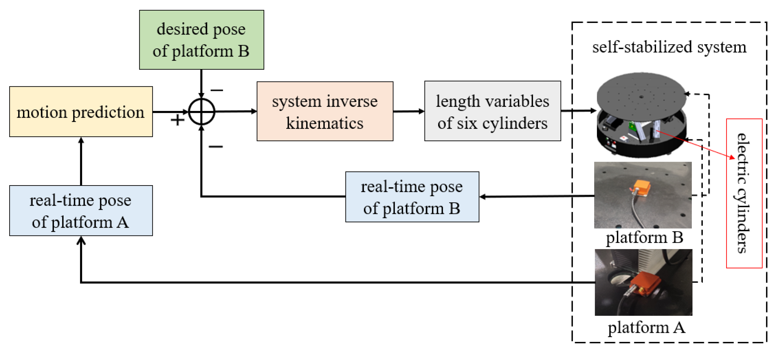
can be calculated by Equation (15). In the meantime, new observation data were continuously obtained by the onboard inertial measurement unit (IMU) during the prediction, and the parameters of the autoregression model could be updated in real-time by the limited memory recursive least squares method.
x ^ t + l = i = 1 p φ i x t + l i         l = 1 i = 1 l 1 φ i x ^ t + l i + i = l p φ i x t + l i       ( 1 < l p ) i = 1 p φ i x ^ t + l i       ( l > p )

3. Self-Stabilized System Design

A Self-Stabilized system was designed by a group of parallel electric cylinders in this section. Meanwhile, a controller based on inverse kinematics was also presented for the Self-Stabilized system. The controller took real-time measurements and predictions of the ship’s attitude as the input was used to compensate for the sway motion of the ship and to keep the constant attitude of the Self-Stabilized system.

3.1. Inverse Kinematics Modeling

The structure of the Self-Stabilized system is shown in Figure 2. Two platforms and six parallel electric cylinders between them comprise the system. The lower platform A was assumed to be fixed to the deck and sways with the hull. The attitude of the upper platform B can be controlled by collaboratively adjusting the lengths of the six electric cylinders.
The pose of the platform B in the coordinate system A can be described as follows:
x = x ,   y ,   z ,   α ,   β ,   γ T
where x , y and z are the origin position of the coordinate system B relative to the coordinate system A . α , β and γ are the Euler or azimuth angle of B . According to the structural diagram of the parallel self-stabilization system, the positions of each hinge point a i and b i   i = 1 ,   2 ,   · · · ,   6 in the respective coordinate system are known. Assuming that the relative pose of platform B is P B A , R B A , R B A is the rotation matrix of the coordinate system B relative to the coordinate system A , and P B A is the corresponding displacement vector. The coordinate of each hinge point b i in the coordinate system A can be calculated as follows:
b A i = R A B b i + P A B , i = 1 , 2 , · · · , 6
As a result, the lengths of all-electric cylinders can be expressed in the coordinate system A as follows:
l i = R A B b i + P A B a i ,     i = 1 , 2 , · · · , 6
The above equation is called the inverse kinematics of the Self-Stabilized system. Relying on the equation, platform B can keep a stable pose relative to platform A by changing the lengths of the six cylinders.

3.2. Motion Compensation Control

A closed-loop control strategy based on attitude feedback was introduced for the self-stability system. As shown in Figure 3, two components are involved: in the first component, real-time ship motion measurements are acquired by the onboard IMU of the lower platform A. To mitigate the hysteresis of the system, the prediction method proposed in Section 2 utilizes the measurements to calculate the motion state the next time in advance. The predictions are used as the feedback input to the controller. In the other component, the pose of the upper platform B after motion compensation can be also obtained by another onboard IMU, which is installed on the upper platform B. The difference between the measured pose and the desired pose of the upper platform B is used as the feedback variable of the closed-loop controller. Thereinto, the sum of the difference and the predicted pose of platform B is regarded as the input of the inverse kinematics module to calculate the length variable of each electric cylinder. In such a way, the system achieves the purpose of self-stabilization.

4. Experiments and Analysis

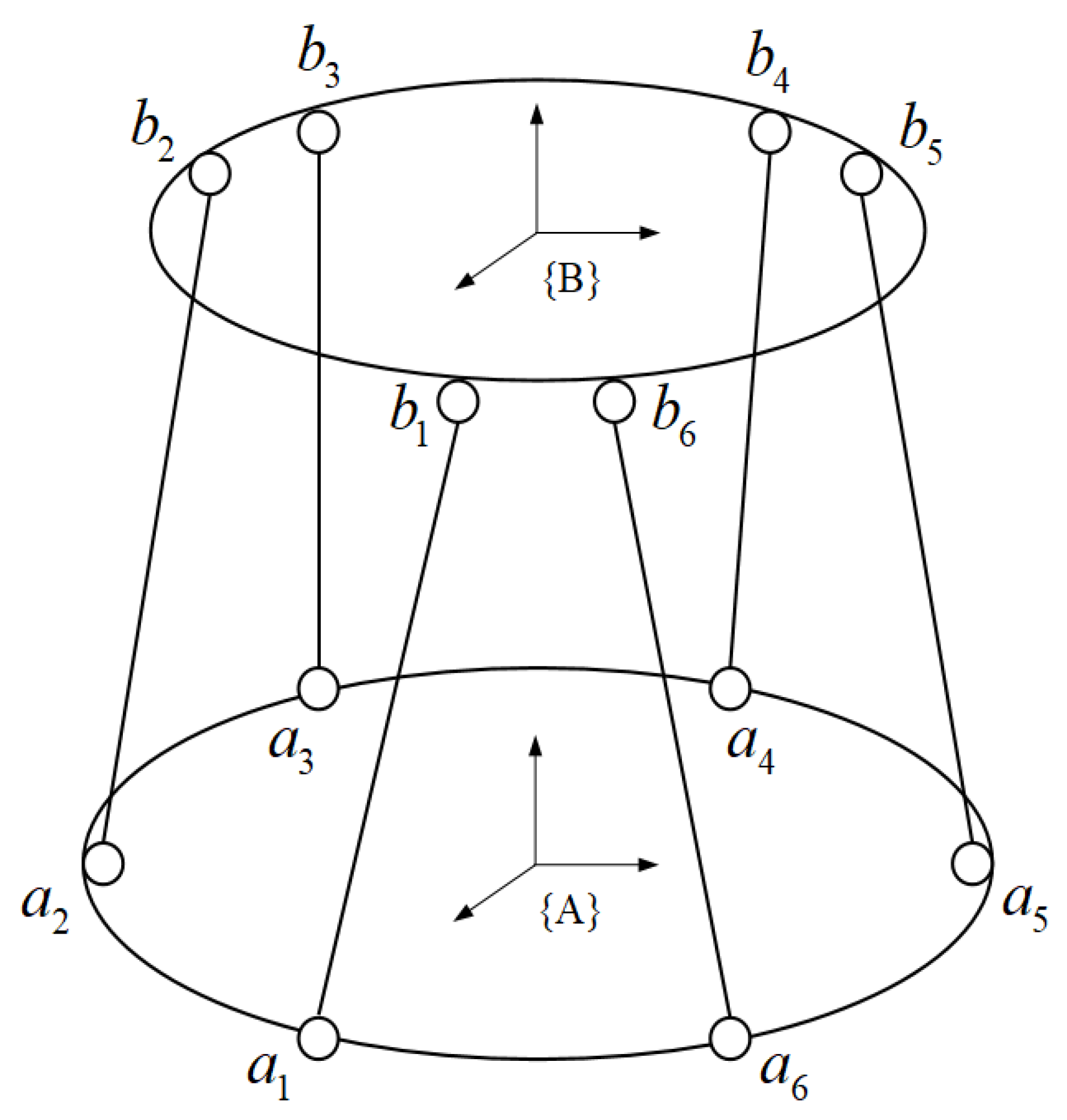
The Self-Stabilized system designed in this work adopts the Stewart mechanism. The position and attitude of the end actuator (platform B) are controlled by six electric cylinders connected to the base (platform A). One end of each electric cylinder is connected to the base with a 2-DOF universal joint, and the other end is connected to the end actuator with a 3-DOF spherical joint. Platform A simulates the ship’s motion through a traditional ship motion model presented in Section 2.1, while platform B is controlled to keep a constant attitude through the Self-Stabilized controller. Both platforms A and B are equipped with high-performance inertial sensors (XSENSE MTi-G-710, https://www.movella.com/products/sensor-modules/xsens-mti-7-gnss-ins#specs, accessed on 29 March 2023). The sensor is a fully integrated solution that includes an onboard GNSS receiver and a full gyro-enhanced attitude and heading reference system. An enhanced 3D pose and velocity are given. For example, the root mean square error (RMSE) of the roll/pitch angle is 0.6 deg while the yaw angle is 1.5 deg. The sensor performs high-speed dead-reckoning calculations at 1000 Hz allowing the accurate capture of high-frequency motions.

4.1. Motion Prediction

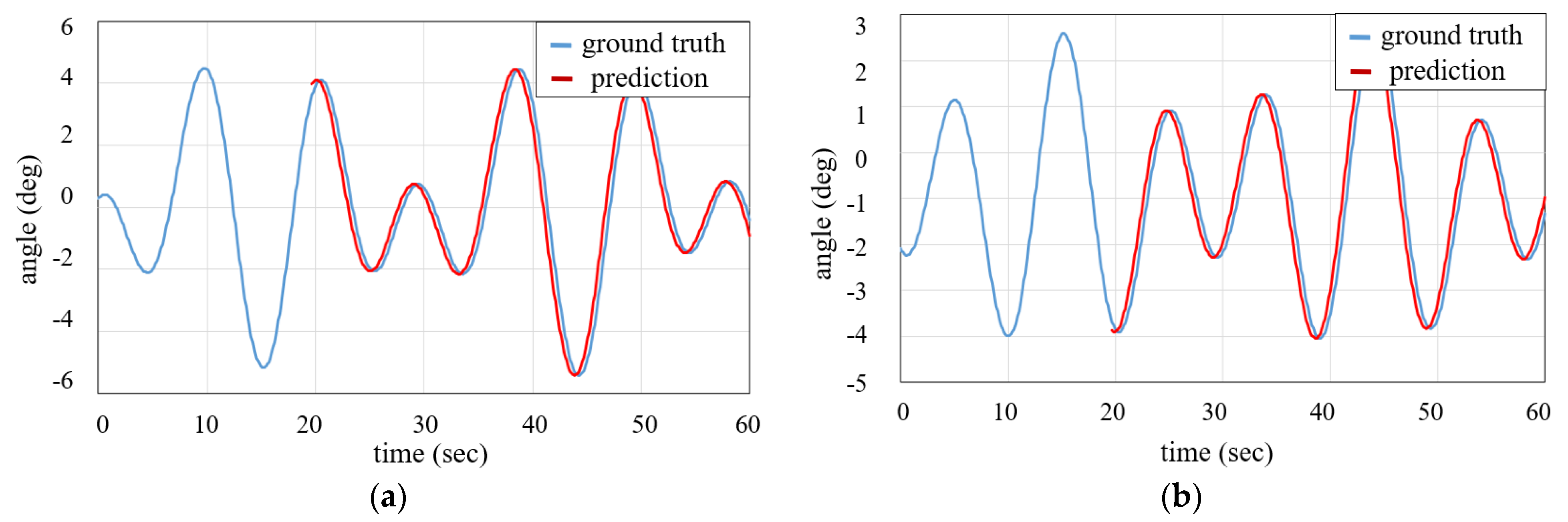
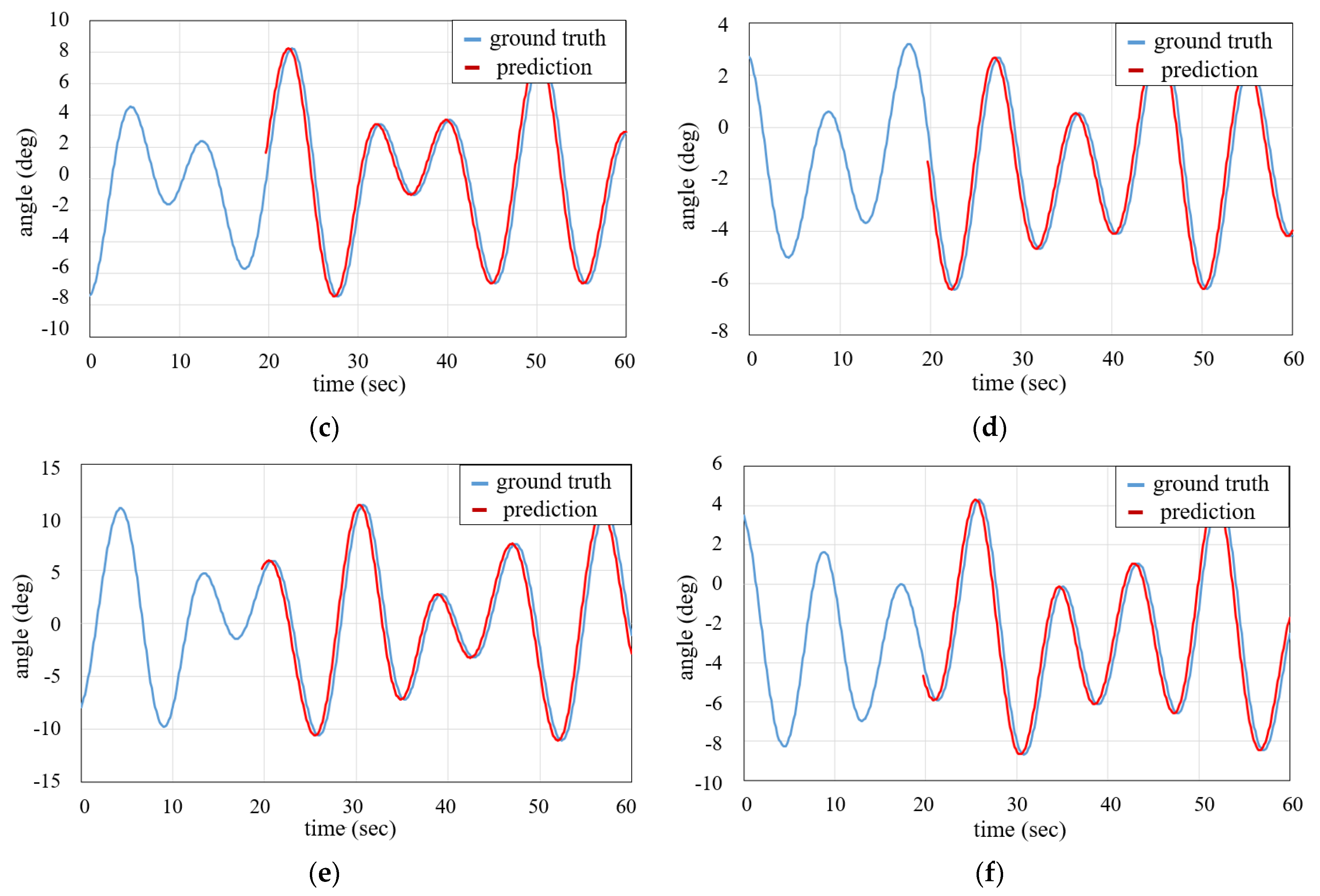
To simulate ship motion at sea, Fossen’s 6-DOF dynamic model was applied, which includes swaying, surging, heaving, rolling, pitch and yaw motions in the 3D position and attitude. The effectiveness of the proposed ship motion prediction method was illustrated by comparing the acquired predictions with the simulation data.
As shown in Figure 4, the ship motions in class 3–5 sea conditions are simulated, respectively. The higher the sea condition class, the more severe the changes in the roll angle and pitch angle. Using the roll and pitch angle data of the previous 20 s as the sample, the parameters of the proposed prediction model are initialized. Then, the model parameters are updated with real-time data. The prediction results are given in Figure 4. Even for the under Class 5 sea condition, the prediction of the pitch and roll angle changes are approximatively consistent with the ground truth. The corresponding errors were calculated and are given in Table 1. The prediction error rates of roll and pitch angle at class 3 were 0.581% and 0.543%, respectively. The prediction error rates of roll and pitch angle at class 5 were 0.733% and 0.922%, respectively. It can be seen that the maximum prediction error of the proposed method was less than 1%. The proposed method was able to help the realization of the offshore Self-Stabilized system.

4.2. Compensation Control

The Self-Stabilized system and its compensation control method were tested by two experimental setups. Due to the limitation of the driving device in the experiments, only the pitch and roll angles of platform A changed over time. In future work, platform A’s motion should be extended in displacement and yaw directions, and control compensation of other DOFs needs to be carried out to illustrate the performance of the Self-Stabilized system.
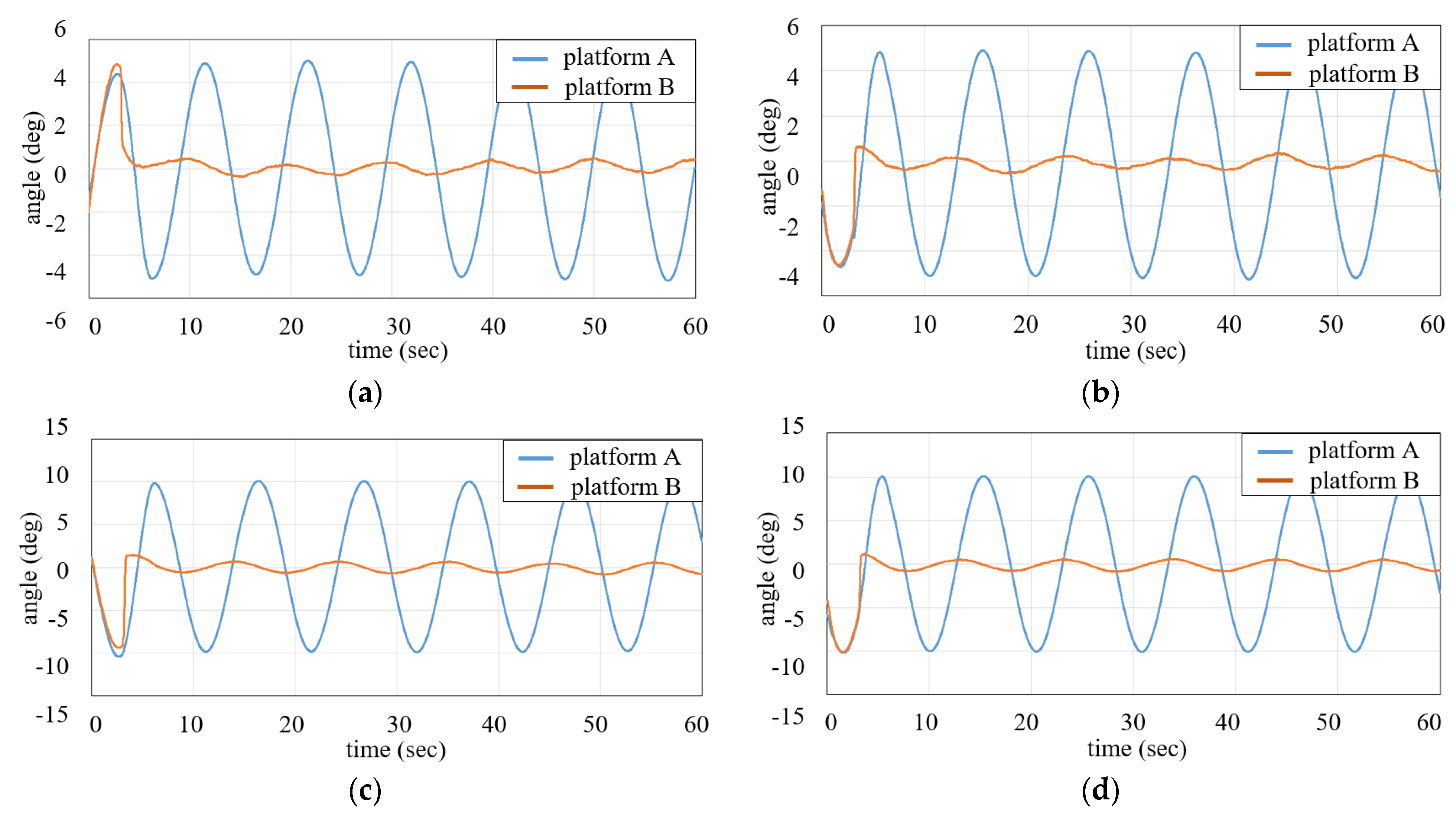
Firstly, the proposed control method was verified by straightforward 1-DOF motion compensation. Platform A simulated the motion of a ship by the driving of a sine function. Through the proposed control method in Section 3, platform B of the Self-Stabilized system could compensate for the motion of platform A. Through the motion compensation, the real-time attitude variations of platforms A and B are shown in Figure 5. When the roll angle changed with an amplitude of 10 deg and a period of 0.1hz, the maximum error of the controller was 0.82 deg, and the mean error was 0.4 deg. The corresponding errors are calculated in Table 2. It can be found that the maximum error of the proposed controller was no more than 1 deg while the mean error was limited to 0.5 deg.
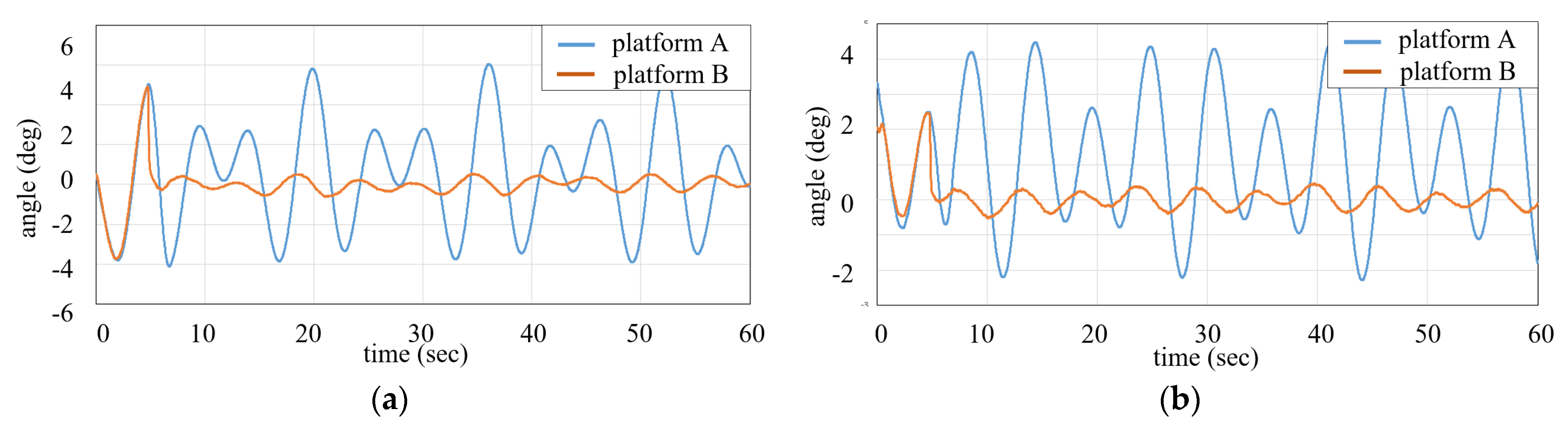
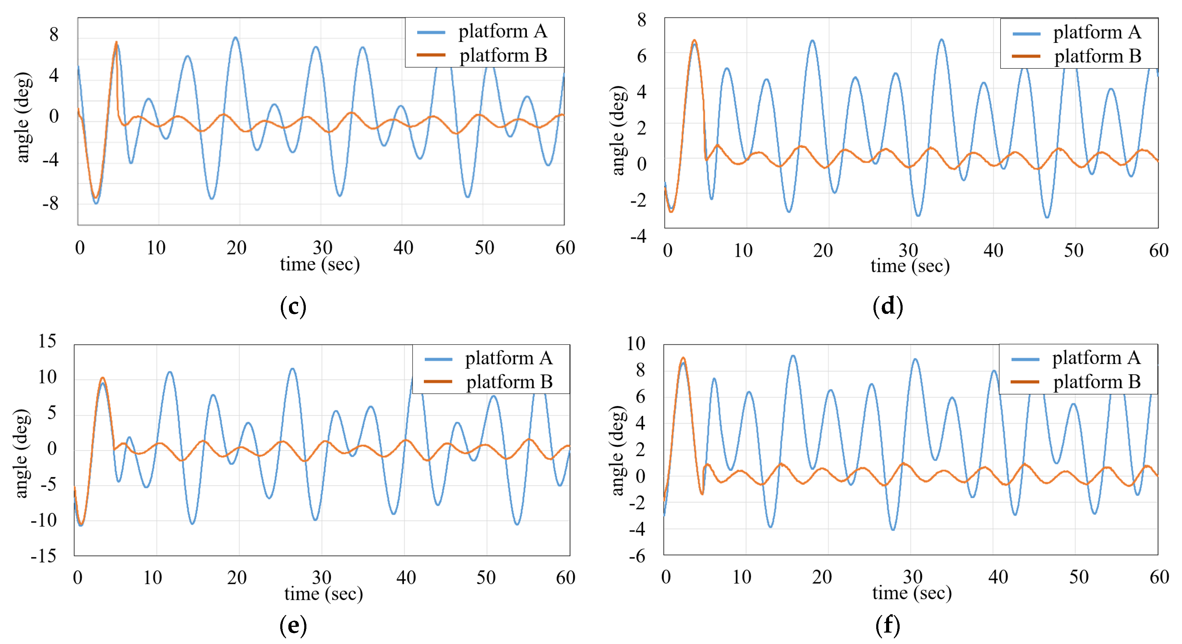
Subsequently, the Self-Stabilized system with the proposed control method was applied close to real experiments. The ship’s motion was simulated in different sea conditions by changing the pitch and roll angles simultaneously with random amplitudes. The response of the Self-Stabilized system is shown in Figure 6. The corresponding errors were calculated and are given in Table 3. The mean errors at class 3 rolling and pitching were 0.25 deg and 0.19 deg, respectively. The maximum errors at class 5 rolling and pitching were 1.6 deg and 0.96 deg, respectively. In one word, the maximum control error of the self-stabilization system was less than 2 deg, and the average error was stable within 1 deg. The control accuracy of the Self-Stabilized system was acceptable.

5. Conclusions

A novel offshore Self-Stabilized system and its motion prediction and compensation control method are presented in this paper. The autoregression model was applied to approximate the ship’s motion when exposed to complex maritime environments. The parameters of the model could be initialized and updated online. Taking the predictions and real-time measurements as the input, the compensation controller achieved the self-stabilization of the system. It was proved by quantitative experiments that the Self-Stabilized system could predict and compensate for the swaying component of the ship’s motion even in complex sea conditions. This system is of great value for shipboard, ship-shore and shipboard–shipboard operations with high precision requirements, such as the takeoff and landing of drones, ship-borne cranes, anti-seasickness seats, etc. In future work, the self-stabilization system should be evaluated in a completely realistic water environment and specific shipboard automated operations.

Author Contributions

Conceptualization, H.Y. and C.X.; methodology, Y.L., Z.X. and C.X.; software, Y.L. and Z.X.; validation, Y.L. and Z.X.; formal analysis, Y.L. and Z.X.; investigation, H.Y. and C.X.; resources, C.X.; data curation, Z.X.; writing—original draft preparation, Y.L.; writing—review and editing, H.Y. and C.X.; visualization, Y.L.; supervision, H.Y.; project administration, H.Y.; funding acquisition, H.Y. All authors have read and agreed to the published version of the manuscript.

Funding

This research was funded by National Natural Science Foundation of China, grant number 52001235; Hubei Provincial Natural Science Foundation, grant number 2022CBF313; Shandong Provincial Natural Science Foundation, grant number ZR2020KE029; Scientific Research Project of Hubei Education Department, grant number D20201501; Youth Science Foundation of WIT, grant number 000017/19QD07.

Institutional Review Board Statement

Not applicable.

Informed Consent Statement

Not applicable.

Data Availability Statement

Not applicable.

Conflicts of Interest

The authors declare no conflict of interest.

References

  1. Chen, D.; Fan, T.; Yuan, H.; Yan, X. The Current Situation and Prospect of Inland River Shipping System Supervision Technology. Transp. Syst. Eng. Inf. 2022, 22, 1–14. [Google Scholar]
  2. Qiao, D.; Liu, G.; Lv, T.; Li, W.; Zhang, J. Marine vision-based situational awareness using discriminative deep learning: A survey. J. Mar. Sci. Eng. 2021, 9, 397. [Google Scholar] [CrossRef]
  3. Zhou, W.; Chen, W.; Liu, H.; Li, X. A New Forward Kinematic Algorithm for a General Stewart Platform. Mech. Mach. Theory. 2015, 87, 177–190. [Google Scholar] [CrossRef]
  4. Liu, P.; Kouguchi, N.; Li, Y. Velocity Measurement of Coherent Doppler Sonar Assisted by Frequency Shift, Kalman Filter and Linear Prediction. J. Mar. Sci. Eng. 2021, 9, 109. [Google Scholar] [CrossRef]
  5. Yuan, H.; Xiao, C.; Wang, Y.; Peng, X.; Wen, Y. Maritime Vessel Emission Monitoring by an UAV Gas Sensor System. Ocean Eng. 2020, 218, 108206. [Google Scholar] [CrossRef]
  6. Che, Z.G.; Chiang, T.A.; Che, Z.H. Feed-forward neural networks training: A comparison between genetic algorithm and back-propagation learning algorithm. Int. J. Innov. Comput. Inf. Control 2011, 7, 5839–5850. [Google Scholar]
  7. Tang, G.; Lei, J.; Du, H.; Yao, B.; Zhu, W.; Hu, X. Proportional-Integral-Derivative Controller Optimization by Particle Swarm Optimization and Back Propagation Neural Network for a Parallel Stabilized Platform in Marine Operations. J. Ocean Eng. Sci. 2022, in press. [Google Scholar] [CrossRef]
  8. Zhu, L.; Li, T. Observer-Based Autopilot Heading Finite-Time Control Design for Intelligent Ship with Prescribed Performance. J. Mar. Sci. Eng. 2021, 9, 828. [Google Scholar] [CrossRef]
  9. Qiang, H.; Jin, S.; Feng, X.; Xue, D.; Zhang, L. Model Predictive Control of a Shipborne Hydraulic Parallel Stabilized Platform based on Ship Motion Prediction. IEEE Access 2020, 8, 181880–181892. [Google Scholar] [CrossRef]
  10. Skulstad, R.; Li, G.; Fossen, T.I.; Vik, B.; Zhang, H. A Hybrid Approach to Motion Prediction for Ship Docking—Integration of a Neural Network Model Into the Ship Dynamic Model. IEEE Trans. Instrum. Meas. 2021, 70, 2501311. [Google Scholar] [CrossRef]
  11. Liu, X.; Yuan, H.; Xiao, C.; Wang, Y.; Yu, Q. Hybrid-driven Vessel Trajectory Prediction based on Uncertainty Fusion. Ocean Eng. 2022, 248, 110836. [Google Scholar] [CrossRef]
  12. Chu, Y.; Li, G.; Zhang, H. Incorporation of Ship Motion Prediction into Active Heave Compensation for Offshore Crane Operation. In Proceedings of the 2020 15th IEEE Conference on Industrial Electronics and Applications (ICIEA), Kristiansand, Norway, 9–13 November 2020; pp. 1444–1449. [Google Scholar]
  13. Zhang, T.; Zheng, X.; Liu, M. Multiscale Attention-based LSTM for Ship Motion Prediction. Ocean Eng. 2021, 230, 109066. [Google Scholar] [CrossRef]
  14. Fu, H.; Gu, Z.; Wang, Y. Ship Pitch Prediction based on Bi–ConvLSTM–CA Model. J. Mar. Sci. Eng. 2022, 10, 840. [Google Scholar] [CrossRef]
  15. Guo, X.; Zhang, X.; Lu, W.; Tian, X.; Li, X. Real-time Prediction of 6–DOF Motions of a Turret-moored FPSO in Harsh Sea State. Ocean Eng. 2022, 265, 112500. [Google Scholar] [CrossRef]
  16. Ren, Z.; Han, X.; Yu, X.; Skjetne, R.; Leira, B.J.; Sævik, S.; Zhu, M. Data–driven Simultaneous Identification of the 6DOF Dynamic Model and Wave Load for a Ship in Waves. Mech. Syst. Signal Process. 2023, 184, 109422. [Google Scholar] [CrossRef]
  17. Yang, X. Displacement Motion Prediction of a Landing Deck for Recovery Operations of Rotary UAVs. Int. J. Control Autom. Syst. 2013, 11, 58–64. [Google Scholar] [CrossRef]
  18. Wei, Y.; Chen, Z.; Zhao, C.; Chen, X. Deterministic Ship Roll Forecasting Model based on Multi-objective Data Fusion and Multi-layer Error Correction. Appl. Soft Comput. 2023, 132, 109915. [Google Scholar] [CrossRef]
  19. Zhao, X.; Zhao, T.; Wang, C.; Xin, T.; Yuhang, C. Type synthesis and analysis of parallel mechanisms with sub-closed-loops. Mech. Mach. Theory 2018, 120, 140–165. [Google Scholar] [CrossRef]
  20. Tian, W.; Zhang, X.; Lv, D.; Wang, L.; Liu, Q. Sliding Mode Control Strategy of 3–UPS/S Shipborne Stable Platform with LSTM Neural Network Prediction. Ocean Eng. 2022, 265, 112497. [Google Scholar] [CrossRef]
  21. Chu, Y.; Li, G.; Hatledal, L.I.; Holmeset, F.T.; Zhang, H. Coupling of Dynamic Reaction Forces of a Heavy Load Crane and Ship Motion Responses in Waves. Ships Offshore Struct. 2021, 16 (Suppl. S1), 58–67. [Google Scholar] [CrossRef]
  22. Chen, H.; Xie, J.; Han, J.; Shi, W.; Charpentier, J.-F.; Benbouzid, M. Position Control of Heave Compensation for Offshore Cranes based on a Particle Swarm Optimized Model Predictive Trajectory Path Controller. J. Mar. Sci. Eng. 2022, 10, 1427. [Google Scholar] [CrossRef]
  23. Bozkurt, B.; Ertogan, M. Heave and Horizontal Displacement and Anti–sway Control of Payload during Ship-to-ship Load Transfer with an Offshore Crane on Very Rough Sea Conditions. Ocean Eng. 2023, 267, 113309. [Google Scholar] [CrossRef]
  24. Xiao, J. Ship Dynamic Positioning Control based on Nonlinear Fuzzy Algorithm for a Smart Port City. J. Test. Eval. 2022, 10, 865. [Google Scholar] [CrossRef]
  25. Sumnu, A.; Guzelbey, I.H.; Cakir, M.V. Simulation and PID Control of a Stewart Platform with Linear Motor. J. Mech. Sci. Technol. 2017, 31, 345–356. [Google Scholar] [CrossRef]
  26. Meng, J.; Humme, A.; Bucknall, R.; Englot, B.; Liu, Y. A Fully Autonomous Framework of Unmanned Surface Vehicles in Maritime Environments Using Gaussian Process Motion Planning. IEEE J. Ocean. Eng. 2022, 48, 59–79. [Google Scholar] [CrossRef]
  27. Dong, Z.; Zhang, Z.; Qi, S.; Zhang, H.; Li, J.; Liu, Y. Autonomous Cooperative Formation Control of Underactuated USVs based on Improved MPC in complex ocean environment. Ocean Eng. 2023, 270, 113633. [Google Scholar] [CrossRef]
Figure 1. Parameter identification and multistep prediction based on the autoregression model of ship motion.
Jmse 11 00745 g001
Figure 2. Diagram of the parallel Self-Stabilized system.
Jmse 11 00745 g002
Figure 3. Motion compensation control method of the Self-Stabilized system.
Jmse 11 00745 g003
Figure 4. Motion prediction of a ship in class 3–5 sea conditions. (a) Class 3 rolling; (b) Class 3 pitching; (c) Class 4 rolling; (d) Class 4 pitching; (e) Class 5 rolling; (f) Class 5 pitching.
Jmse 11 00745 g004aJmse 11 00745 g004b
Figure 5. Self−stabilization in 1DOF sin motion condition. (a) Roll angle   5 deg; (b) Pitch angle   5 deg; (c) Roll angle   10 deg; (d) Pitch angle   10 deg.
Jmse 11 00745 g005
Figure 6. Self-Stabilized control in 3–5 level sea conditions. (a) Class 3 rolling; (b) Class 3 pitching; (c) Class 4 rolling; (d) Class 4 pitching; (e) Class 5 rolling; (f) Class 5 pitching.
Jmse 11 00745 g006aJmse 11 00745 g006b
Table 1. Error statistics of ship motion prediction in class 3–5 sea conditions (%).
Class 3Class 4Class 5
Roll0.5810.6580.733
Pitch0.5430.5770.922
Table 2. Self-stabilization control errors in 1DOF motion conditions.
1-DOF MotionMaximum Error (deg)Mean Error (deg)
roll angle   5 deg0.500.19
roll angle   10 deg0.820.40
pitch angle   5 deg0.550.20
pitch angle   10 deg0.880.42
Table 3. Error analysis of the Self-Stabilized system in 3–5 level sea conditions.
Sea ConditionMaximum Error (deg)Mean Error (deg)
class 3 rolling0.610.25
class 3 pitching0.500.19
class 4 rolling0.850.40
class 4 pitching0.680.29
class 5 rolling1.600.66
class 5 pitching0.960.39
Disclaimer/Publisher’s Note: The statements, opinions and data contained in all publications are solely those of the individual author(s) and contributor(s) and not of MDPI and/or the editor(s). MDPI and/or the editor(s) disclaim responsibility for any injury to people or property resulting from any ideas, methods, instructions or products referred to in the content.

