Application of Synthetic DINCAE–BME Spatiotemporal Interpolation Framework to Reconstruct Chlorophyll–a from Satellite Observations in the Arabian Sea


Abstract
:1. Introduction
2. Materials and Methods
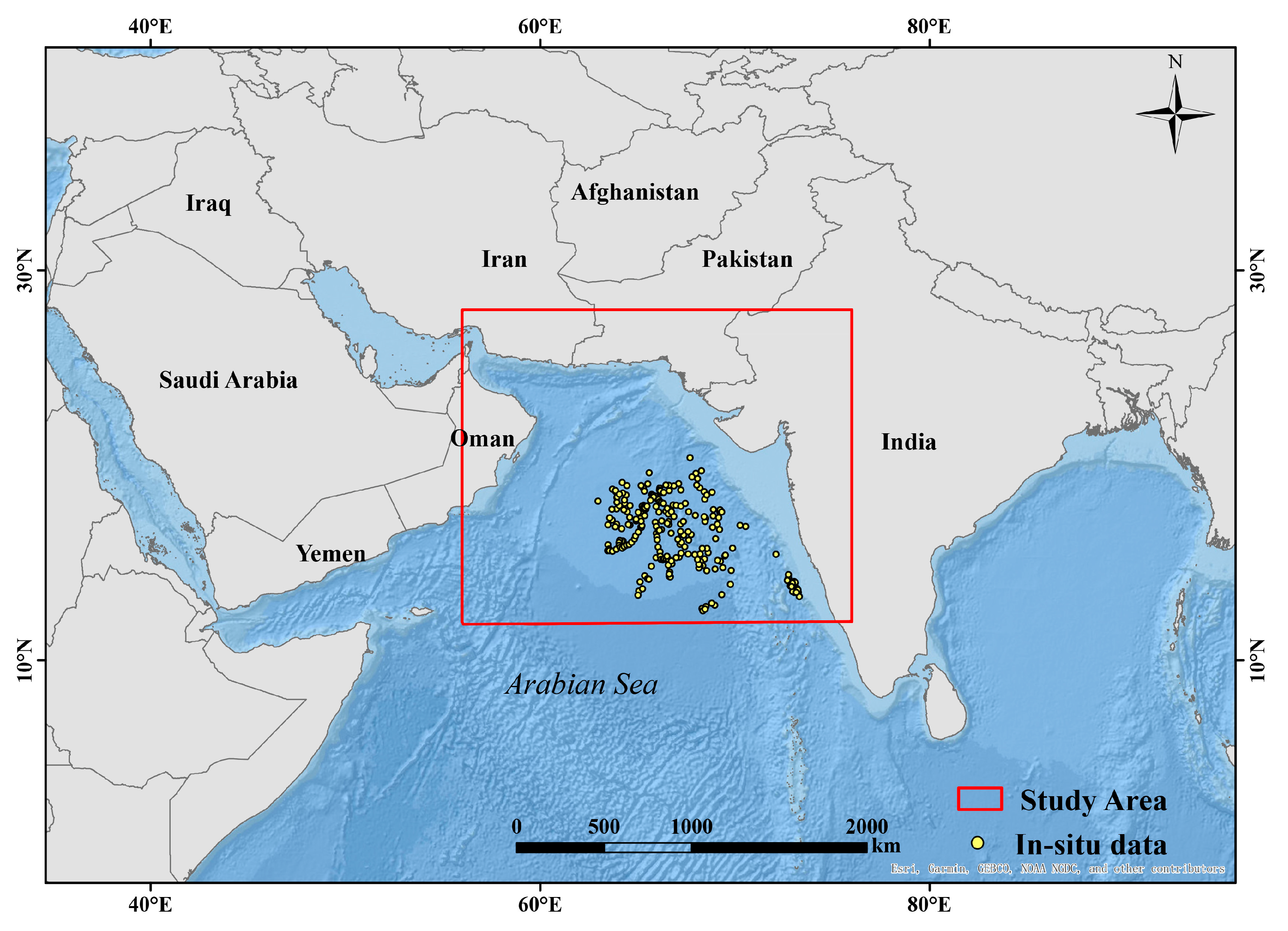
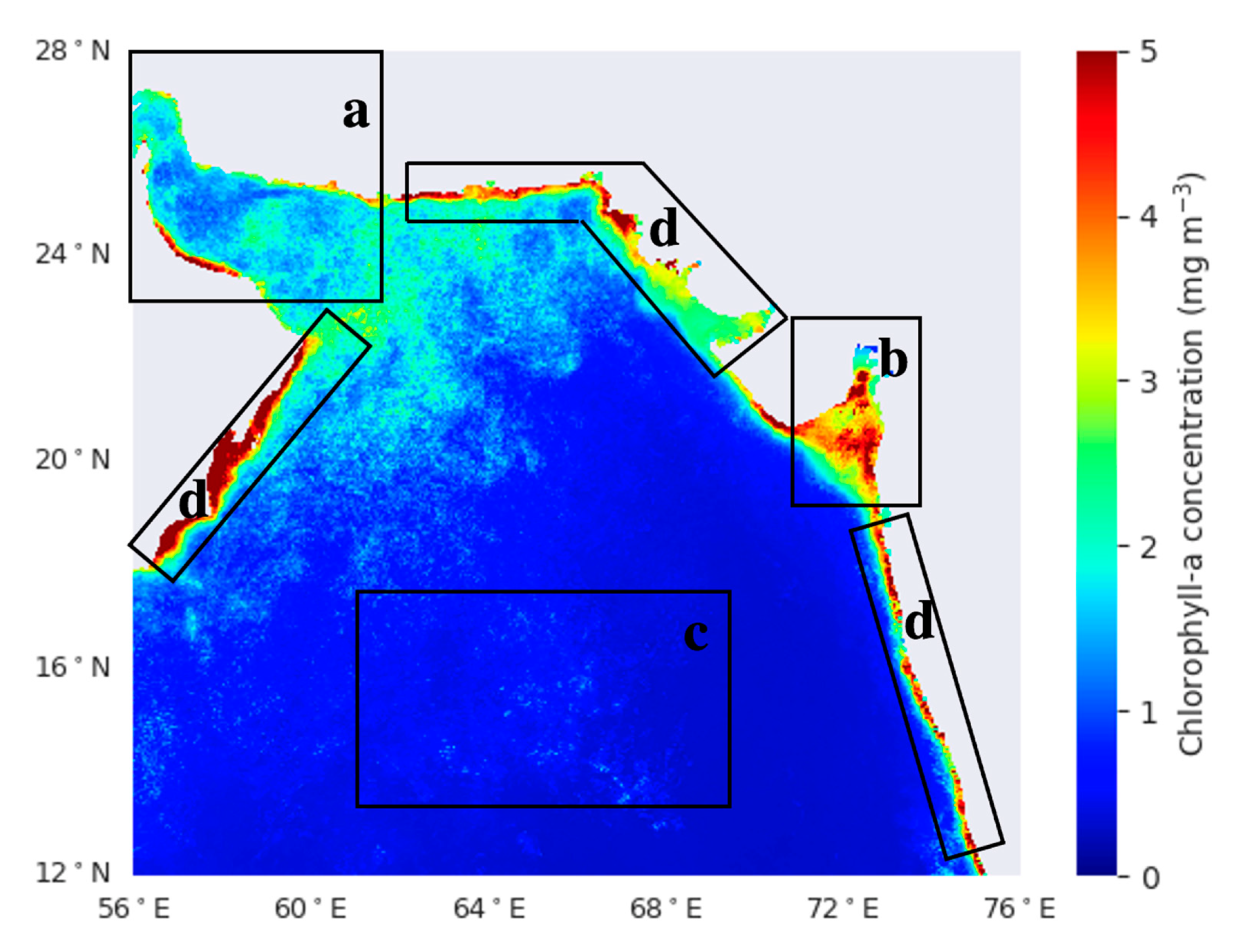
2.1. Study Area
2.2. Satellite Data
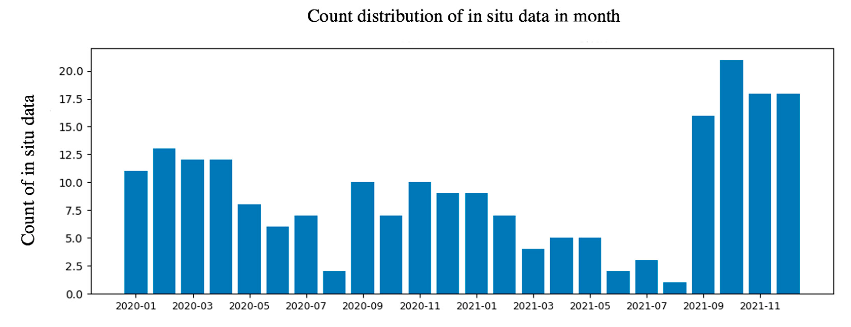
2.3. In Situ Data
2.4. Cross–Validation
2.5. Methods
2.5.1. DINEOF
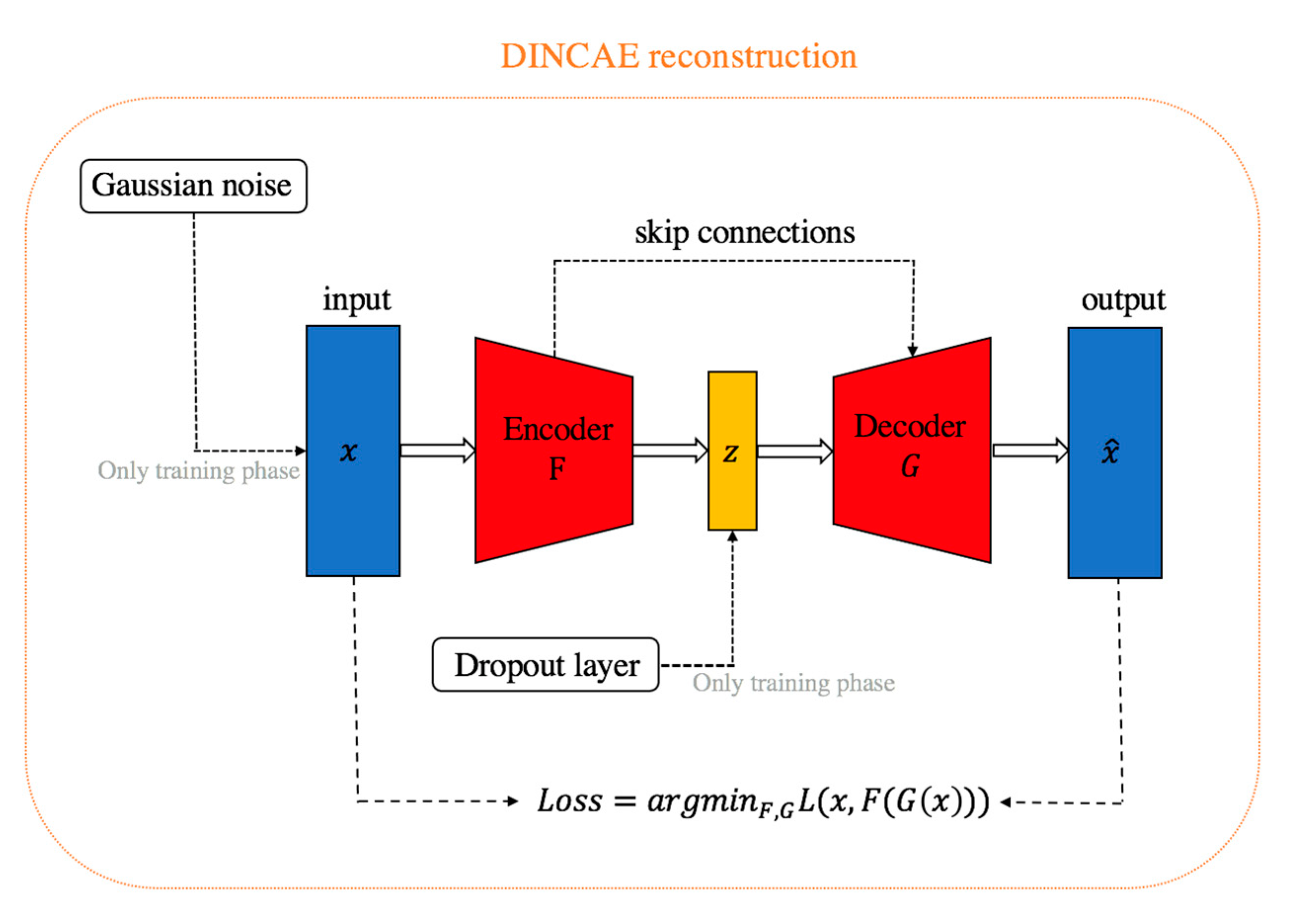
2.5.2. DINCAE
- During the training phase, Gaussian–distributed noise can be added to the input data. With the random noise, the model can address the overfitting problem and its robustness can be boosted;
- Dropout [31], which makes the neural units randomly inactive in a fully connected layer, has proven its effectiveness in solving the overfitting issue in many studies [32]. Similar to the Gaussian–distributed noise, the above method was only implemented in the training phase and disabled during the reconstruction phase;
- The activation function, which is used to enhance the nonlinear fitting capacity of a model, is widely applied after the fully connection layer and convolution layer. The formula for the rectified linear unit (Relu) is as follows:
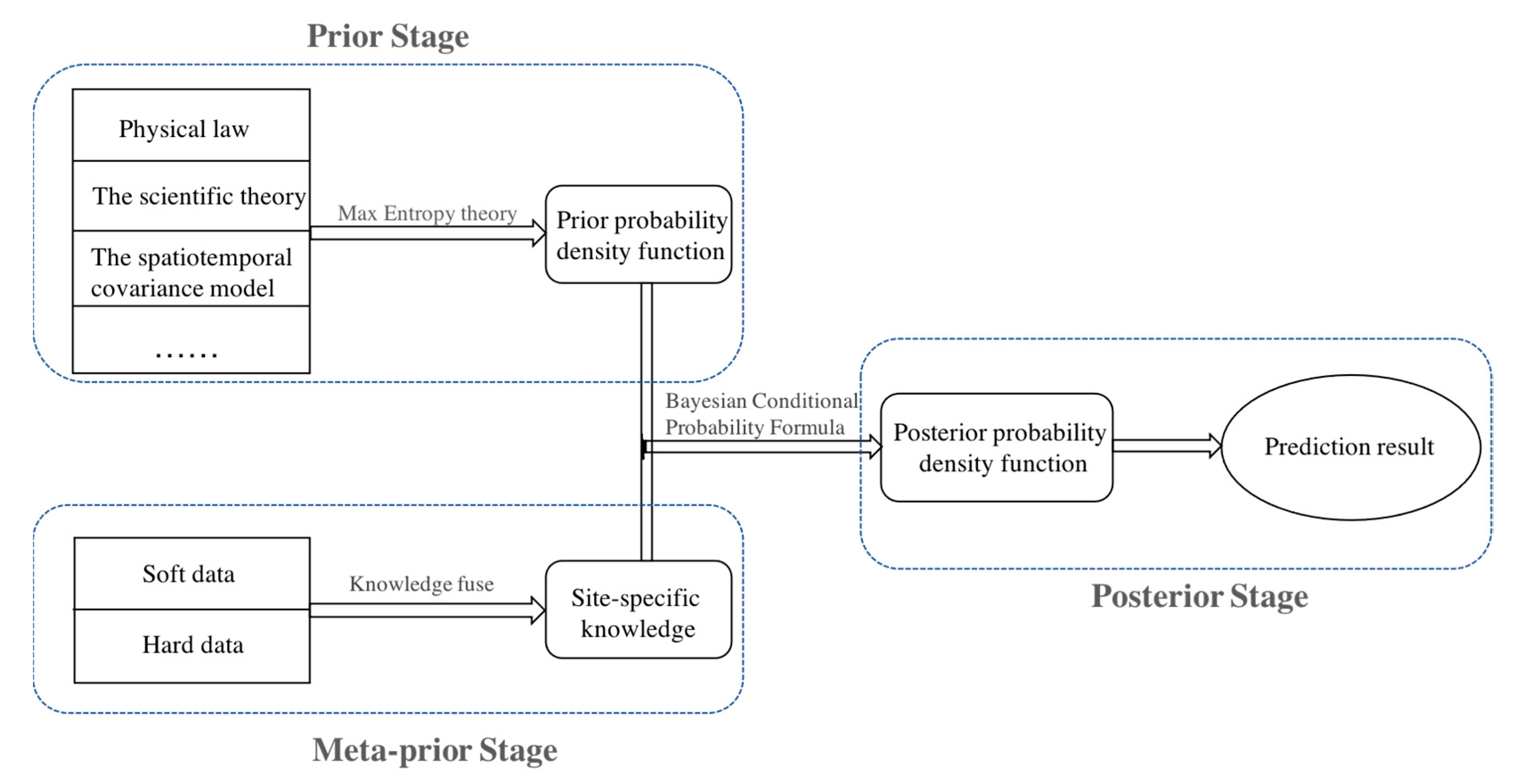
2.5.3. BME
- (a)
- Prior stage. The purpose of the prior stage was to obtain the prior probability density function by using various types of knowledge, such as physical laws, scientific theory, spatiotemporal covariance models, etc. Based on the general knowledge, the constraint equation can be described as the following:
- (b)
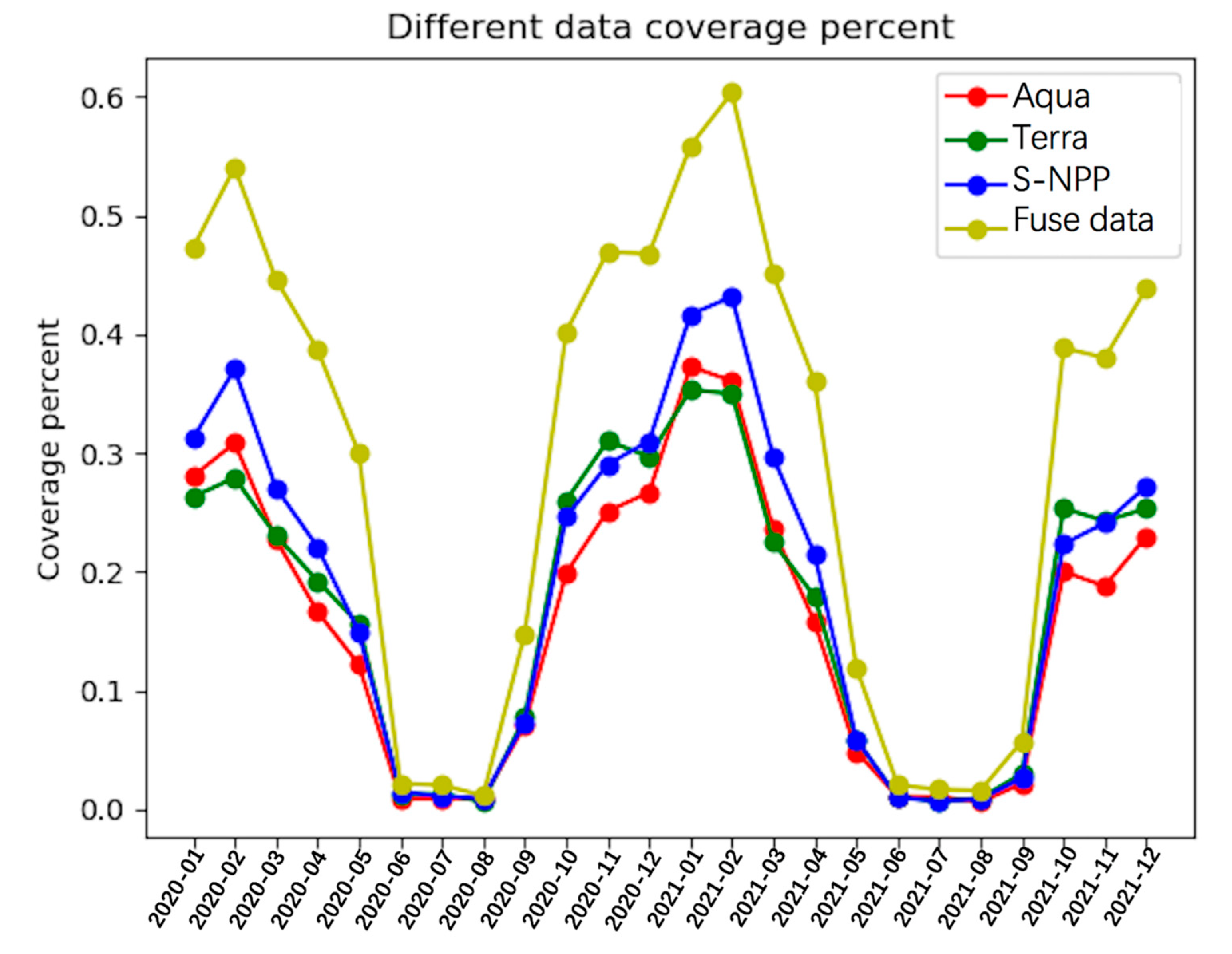
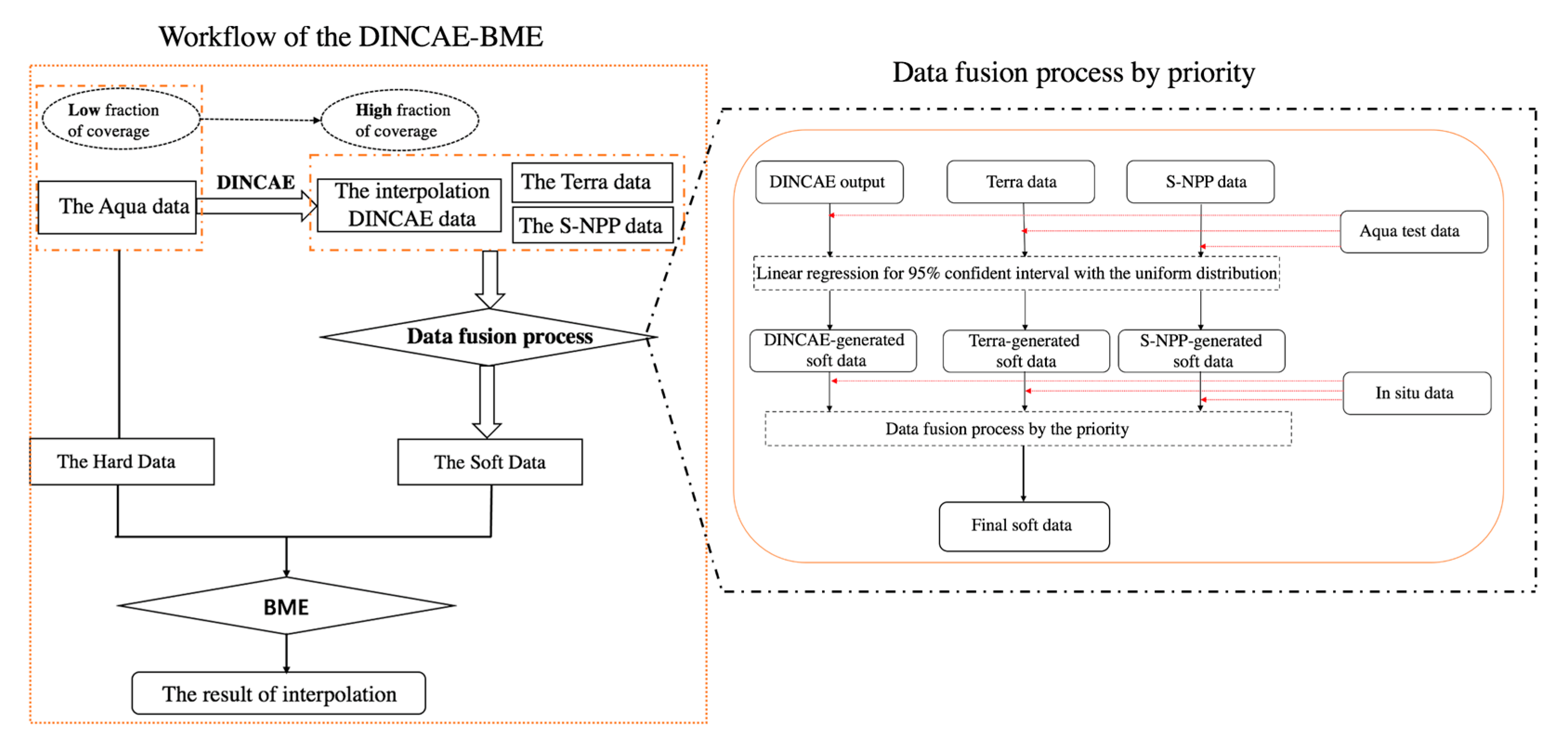
- Meta prior stage. The work in this stage comprised data processing, including hard and soft data preparation. The soft data had inherent uncertainty, such as that in low–precision remote sensing data, and they used three kinds of data formats: the interval format, probability format and function format. In this study, Chl–a data from the Aqua satellite were considered as hard data and used for DINEOF and DINCAE modeling, while the soft data were generated from the DINCAE output data, the original Terra data and the original S–NPP data, as shown in Figure 6.The detailed process was as follows: the matched–up and paired data from the Aqua test dataset and the DINCAE output data/Terra data/S–NPP data were respectively used to build a linear model for calibration; then, all the DINCAE output data/Terra data/S–NPP data were introduced into the corresponding linear model to generate soft Chl–a data with a uniform–distribution probability density function by setting the upper and lower limits of the 95% confidence intervals of the linear models’ outputs as the upper and lower limits of the uniform distribution. The linear regression results are shown in Table 2. Further, the in situ Chl–a data were matched and compared with the linear model output (or estimation) to determine the priority of the soft data strategy chosen from among DINCAE–generated soft data, TERRA–generated soft data and S–NPP–generated soft data. Given that the R2 values of the linear regression models for the in situ data and three kinds of estimations were 0.4661, 0.7246 and 0.6239, the priority for the choice of strategies for the soft data was set as Terra > S–NPP > output of DINCAE. Thus, the hard and soft data were prepared. In this study, the hard and soft data were both used for BME modeling.
- (c)
- Posterior stage. The main purpose of the posterior stage was to obtain the posterior probability distribution by making use of general knowledge, hard data and soft data. The process of determining the posterior probability distribution essentially involved solving the condition probability formula shown in the following equation:
2.5.4. DINCAE–BME Framework
3. Results
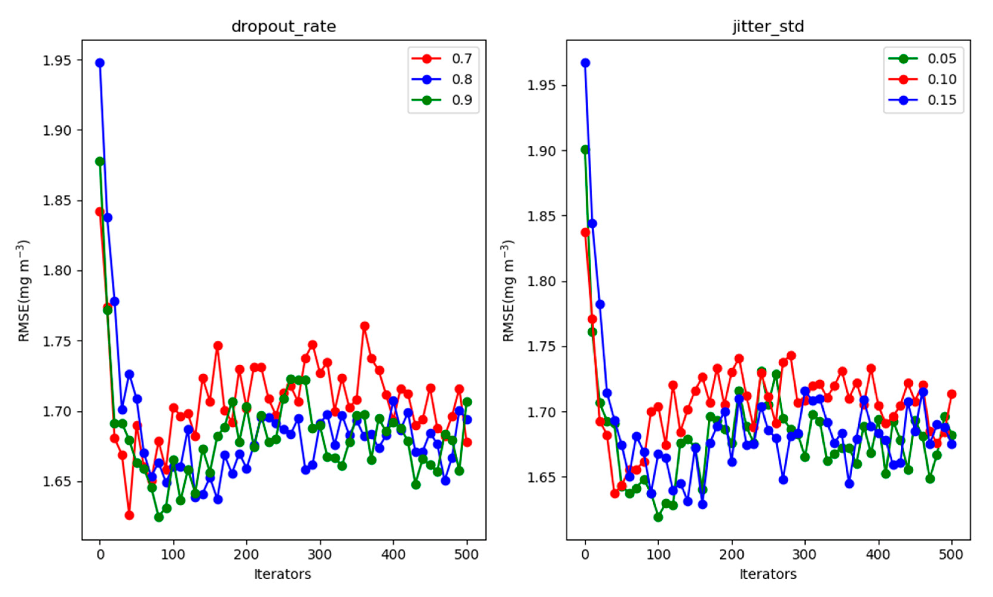
3.1. Hyperparameter Experiment
3.2. Cross–Validation Result
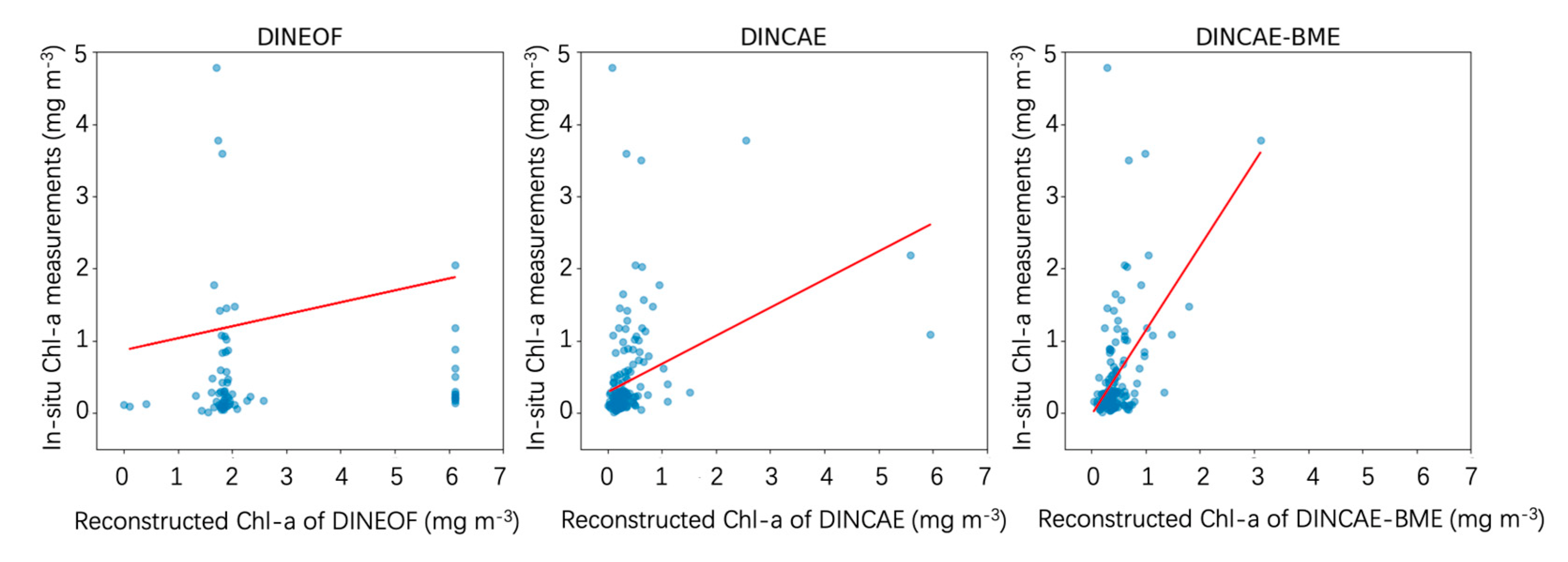
3.3. Validation with the In Situ Data
3.4. Reconstruction Statistics
4. Discussion
4.1. Methodology
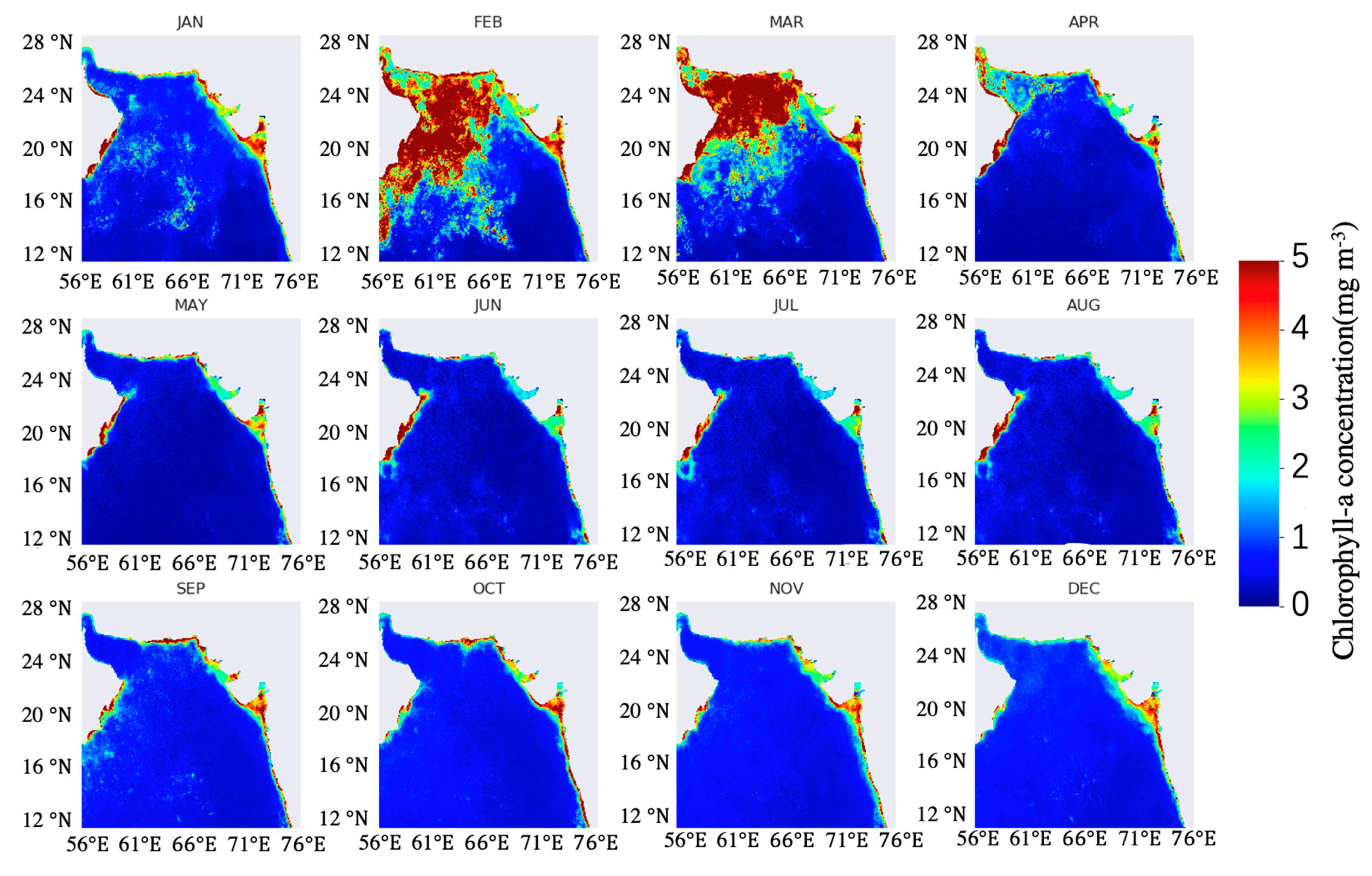
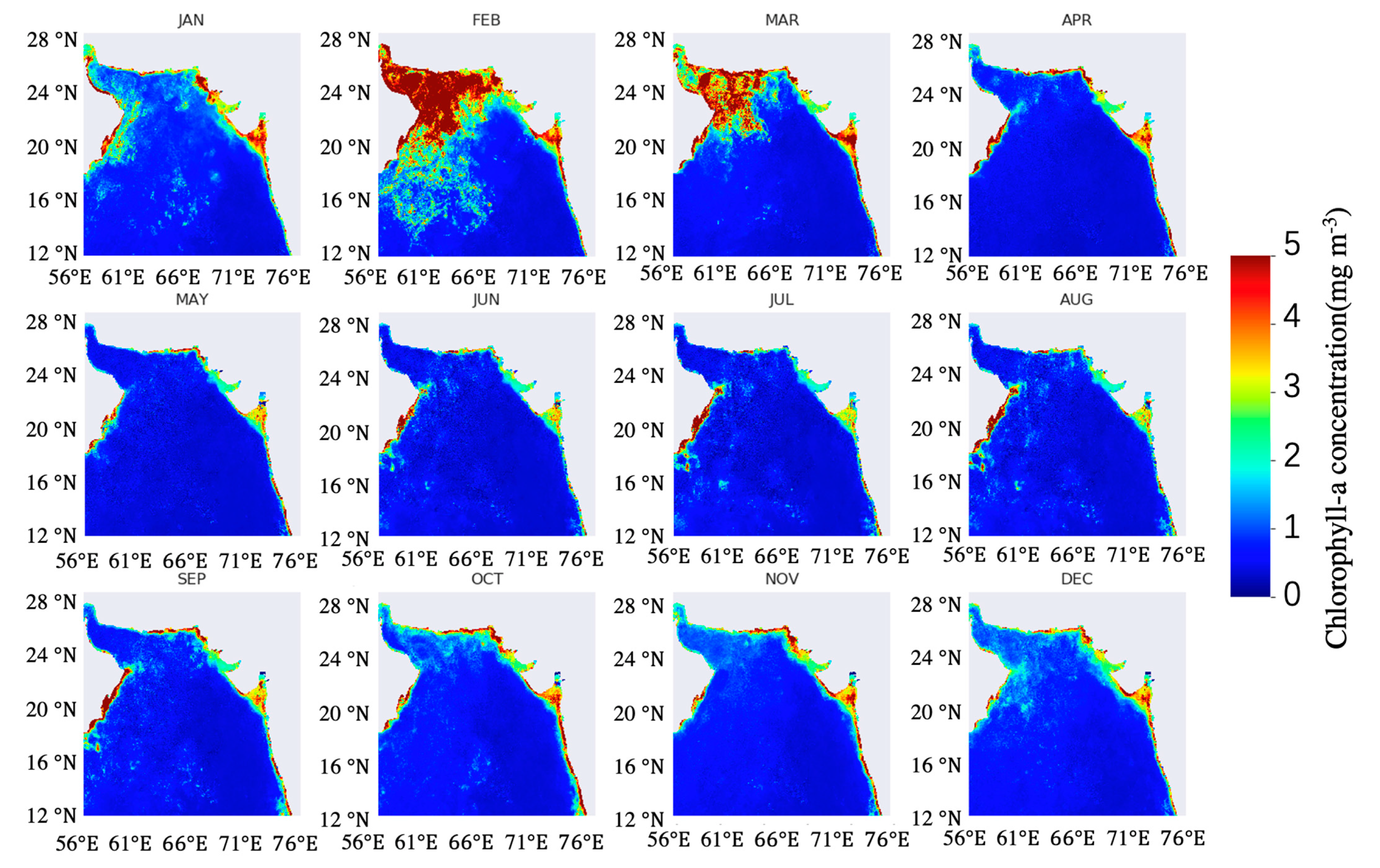
4.2. Product Analysis
5. Conclusions
Author Contributions
Funding
Institutional Review Board Statement
Informed Consent Statement
Data Availability Statement
Conflicts of Interest
References
- He, J.; Chen, Y.; Wu, J.; Stow, D.A.; Christakos, G. Space–Time Chlorophyll–a Retrieval in Optically Complex Waters That Accounts for Remote Sensing and Modeling Uncertainties and Improves Remote Estimation Accuracy. Water Res. 2020, 171, 115403. [Google Scholar] [CrossRef]
- Kasprzak, P.; Padisák, J.; Koschel, R.; Krienitz, L.; Gervais, F. Chlorophyll a Concentration across a Trophic Gradient of Lakes: An Estimator of Phytoplankton Biomass? Limnologica 2008, 38, 327–338. [Google Scholar] [CrossRef] [Green Version]
- Johan, F.; Jafri, M.Z.; Lim, H.S.; Wan Maznah, W.O. Laboratory Measurement: Chlorophyll–a Concentration Measurement with Acetone Method Using Spectrophotometer. In 2014 IEEE International Conference on Industrial Engineering and Engineering Management; IEEE: New York, NY, USA, 2014. [Google Scholar]
- Hamilton, R.J.; Sewell, P.A. Introduction to High Performance Liquid Chromatography; Springer: Dordrecht, The Netherlands, 1982; pp. 1–12. [Google Scholar]
- Xing, X.G.; Zhao, D.Z.; Liu, Y.G.; Yang, J.; Shen, H. Progress in fluorescence remote sensing of chlorophyll–a. J. Remote Sens. 2007, 11, 137–144. [Google Scholar]
- Han, Z.; He, Y.; Liu, G.; Perrie, W. Application of DINCAE to Reconstruct the Gaps in Chlorophyll–a Satellite Observations in the South China Sea and West Philippine Sea. Remote Sens. 2020, 12, 480. [Google Scholar] [CrossRef] [Green Version]
- Everson, R.; Cornillon, P.; Sirovich, L.; Webber, A. An Empirical Eigenfunction Analysis of Sea Surface Temperatures in the Western North Atlantic. J. Phys. Oceanogr. 1997, 27, 468–479. [Google Scholar] [CrossRef]
- Chapman, C.; Charantonis, A.A. Reconstruction of Subsurface Velocities from Satellite Observations Using Iterative Self–Organizing Maps. IEEE Geosci. Remote Sens. Lett. 2017, 14, 617–620. [Google Scholar] [CrossRef]
- Hilborn, A.; Costa, M. Applications of DINEOF to satellite–derived chlorophyll–a from a productive coastal region. Remote Sens. 2018, 10, 1449. [Google Scholar] [CrossRef] [Green Version]
- Jayaram, C.; Priyadarshi, N.; Pavan Kumar, J.; Udaya Bhaskar, T.V.S.; Raju, D.; Kochuparampil, A.J. Analysis of Gap–Free Chlorophyll–a Data from MODIS in Arabian Sea, Reconstructed Using DINEOF. Int. J. Remote Sens. 2018, 39, 7506–7522. [Google Scholar] [CrossRef]
- Wang, Y.; Liu, D. Reconstruction of satellite chlorophyll–a data using a modified DINEOF method: A case study in the Bohai and Yellow seas, China. Int. J. Remote Sens. 2014, 35, 204–217. [Google Scholar] [CrossRef]
- Ji, C.; Zhang, Y.; Cheng, Q.; Tsou, J.; Jiang, T.; Liang, X.S. Evaluating the Impact of Sea Surface Temperature (SST) on Spatial Distribution of Chlorophyll–a Concentration in the East China Sea. Int. J. Appl. Earth Obs. Geoinf. 2018, 68, 252–261. [Google Scholar] [CrossRef]
- Barth, A.; Alvera–Azcárate, A.; Licer, M.; Beckers, J. –M. DINCAE 1.0: A Convolutional Neural Network with Error Estimates to Reconstruct Sea Surface Temperature Satellite Observations. Geosci. Model Dev. 2020, 13, 1609–1622. [Google Scholar] [CrossRef] [Green Version]
- Jung, S.; Yoo, C.; Im, J. High–Resolution Seamless Daily Sea Surface Temperature Based on Satellite Data Fusion and Machine Learning over Kuroshio Extension. Remote Sens. 2022, 14, 575. [Google Scholar] [CrossRef]
- Barth, A.; Alvera–Azcárate, A.; Troupin, C.; Beckers, J.-M. DINCAE 2.0: Multivariate Convolutional Neural Network with Error Estimates to Reconstruct Sea Surface Temperature Satellite and Altimetry Observations. Geosci. Model Dev. 2022, 15, 2183–2196. [Google Scholar] [CrossRef]
- Luo, X.; Song, J.; Guo, J.; Fu, Y.; Wang, L.; Cai, Y. Reconstruction of Chlorophyll–a Satellite Data in Bohai and Yellow Sea Based on DINCAE Method. Int. J. Remote Sens. 2022, 43, 3336–3358. [Google Scholar] [CrossRef]
- Barth, A.; Alvera–Azcarate, A.; Troupin, C.; Beckers, J.-M.; Van der Zande, D. Reconstruction of Missing Data in Satellite Images of the Southern North Sea Using a Convolutional Neural Network (Dincae). In 2021 IEEE International Geoscience and Remote Sensing Symposium IGARSS; IEEE: New York, NY, USA, 2021. [Google Scholar]
- Houyoux, A. Reconstruction of Missing Data in HF Radar Observations Using the Convolutional Autoencoder DINCAE. Master’s Thesis, University of Liège, Liège, Belgium, 2021. [Google Scholar]
- Kostopoulou, E. Applicability of Ordinary Kriging Modeling Techniques for Filling Satellite Data Gaps in Support of Coastal Management. Model. Earth Syst. Environ. 2020, 7, 1145–1158. [Google Scholar] [CrossRef]
- Hou, P.; Luo, Y.; Yang, K.; Shang, C.; Zhou, X. Changing Characteristics of Chlorophyll a in the Context of Internal and External Factors: A Case Study of Dianchi Lake in China. Sustainability 2019, 11, 7242. [Google Scholar] [CrossRef] [Green Version]
- He, J.; Christakos, G.; Wu, J.; Li, M.; Leng, J. Spatiotemporal BME Characterization and Mapping of Sea Surface Chlorophyll in Chesapeake Bay (USA) Using Auxiliary Sea Surface Temperature Data. Sci. Total Environ. 2021, 794, 148670. [Google Scholar] [CrossRef]
- Christakos, G. A Bayesian/Maximum–Entropy View to the Spatial Estimation Problem. Math. Geol. 1990, 22, 763–777. [Google Scholar] [CrossRef]
- Jiang, Y.; Gao, Z.; He, J.; Wu, J.; Christakos, G. Application and Analysis of XCO2 Data from OCO Satellite Using a Synthetic DINEOF–BME Spatiotemporal Interpolation Framework. Remote Sens. 2022, 14, 4422. [Google Scholar] [CrossRef]
- Gao, Z.; Jiang, Y.; He, J.; Wu, J.; Christakos, G. Bayesian Maximum Entropy Interpolation of Sea Surface Temperature Data: A Comparative Assessment. Int. J. Remote Sens. 2022, 43, 148–166. [Google Scholar] [CrossRef]
- He, M.; He, J.; Christakos, G. Improved Space–Time Sea Surface Salinity Mapping in Western Pacific Ocean Using Contingogram Modeling. Stoch. Environ. Res. Risk Assess. 2020, 34, 355–368. [Google Scholar] [CrossRef]
- Lang, Y.; Christakos, G. Ocean Pollution Assessment by Integrating Physical Law and Site-specific Data. Environmetrics 2019, 30, e2547. [Google Scholar] [CrossRef]
- Shafeeque, M.; George, G.; Akash, S.; Smitha, B.R.; Shah, P.; Balchand, A.N. Interannual Variability of Chlorophyll–a and Impact of Extreme Climatic Events in the South Eastern Arabian Sea. Reg. Stud. Mar. Sci. 2021, 48, 101986. [Google Scholar] [CrossRef]
- Shi, W.; Wang, M. Phytoplankton Biomass Dynamics in the Arabian Sea from VIIRS Observations. J. Mar. Syst. 2022, 227, 103670. [Google Scholar] [CrossRef]
- Lei, Q.; Luo, H.; Bai, L. Space–time dynamic changes of aerosols in the Arabian Sea and characteristics of chlorophyll a concentration in the sea area. Chin. J. Ecol. 2019, 39, 3110–3120. [Google Scholar]
- Ronneberger, O.; Fischer, P.; Brox, T. U–Net: Convolutional Networks for Biomedical Image Segmentation. In Lecture Notes in Computer Science; Springer International Publishing: Cham, Switzerland, 2015; pp. 234–241. [Google Scholar]
- Srivastava, N.; Hinton, G.; Krizhevsky, A.; Sutskever, I.; Salakhutdinov, R. Dropout: A simple way to prevent neural networks from overfitting. J. Mach. Learn. Res. 2014, 15, 1929–1958. [Google Scholar]
- Cheng, G.; Peddinti, V.; Povey, D.; Manohar, V.; Khudanpur, S.; Yan, Y. An Exploration of Dropout with LSTMs. In Interspeech 2017; ISCA: Dublin, Ireland, 2017. [Google Scholar]
- Maas, A.L.; Hannun, A.Y.; Ng, A.Y. Rectifier nonlinearities improve neural network acoustic models. In Proceedings of the 30th International Conference on Machine Learning, Atlanta, GA, USA, 16–21 June 2013. [Google Scholar]
- Christakos, G. Random Field Models in Earth Sciences; Dover Publications: Mineola, NY, USA, 2012. [Google Scholar]
- Gernez, P.; Doxaran, D.; Barillé, L. Shellfish Aquaculture from Space: Potential of Sentinel2 to Monitor Tide–Driven Changes in Turbidity, Chlorophyll Concentration and Oyster Physiological Response at the Scale of an Oyster Farm. Front. Mar. Sci. 2017, 4, 137. [Google Scholar] [CrossRef] [Green Version]
- Zhang, H.; Qiu, Z.; Sun, D.; Wang, S.; He, Y. Seasonal and Interannual Variability of Satellite–Derived Chlorophyll–a (2000–2012) in the Bohai Sea, China. Remote Sens. 2017, 9, 582. [Google Scholar] [CrossRef] [Green Version]
- Piontkovski, S.; Al–Azri, A.; Al–Hashmi, K. Seasonal and Interannual Variability of Chlorophyll–a in the Gulf of Oman Compared to the Open Arabian Sea Regions. Int. J. Remote Sens. 2011, 32, 7703–7715. [Google Scholar] [CrossRef]
- Yoder, J.A. An Overview of Temporal and Spatial Patterns in Satellite–Derived Chlorophyll–a Imagery and Their Relation to Ocean Processes. Elsevier Oceanogr. Ser. 2000, 63, 225–238. [Google Scholar]
- Mei, Y.; Li, J.; Xiang, D.; Zhang, J. When a Generalized Linear Model Meets Bayesian Maximum Entropy: A Novel Spatiotemporal Ground–Level Ozone Concentration Retrieval Method. Remote Sens. 2021, 13, 4324. [Google Scholar] [CrossRef]
- Ghaemi, M.; Abtahi, B.; Gholamipour, S. Spatial Distribution of Nutrients and Chlorophyll a across the Persian Gulf and the Gulf of Oman. Ocean Coast. Manag. 2021, 201, 105476. [Google Scholar] [CrossRef]
- Shalin, S.; Samuelsen, A.; Korosov, A.; Menon, N.; Backeberg, B.C.; Pettersson, L.H. Delineation of Marine Ecosystem Zones in the Northern Arabian Sea during Winter. Biogeosciences 2018, 15, 1395–1414. [Google Scholar] [CrossRef] [Green Version]
- Yang, L. Research progress in determination of phytoplankton chlorophyll–a. Sichuan Environ. 2019, 38, 156–160. [Google Scholar]
- Dey, S.; Singh, R.P. Comparison of Chlorophyll Distributions in the Northeastern Arabian Sea and Southern Bay of Bengal Using IRS–P4 Ocean Color Monitor Data. Remote Sens. Environ. 2003, 85, 424–428. [Google Scholar] [CrossRef]
- Naqvi, A.; Narvekar, V.; Desa, E. Coastal biogeochemical processes in the north Indian Ocean (14, S–W). In The Sea: Ideas and Observations on Progress in the Study of the Seas; Robinson, A.R., Brink, K.H., Eds.; Wiley: Hoboken, NJ, USA, 2006; pp. 723–781. [Google Scholar]
- Garcia, E.; Locarnini, A.; Boyer, P.; Antonov, I. Dissolved inorganic nutrients (phosphate, nitrate, silicate). World Ocean. Atlas 2013, 4, 25. [Google Scholar]
- Braga, F.; Ciani, D.; Colella, S.; Organelli, E.; Pitarch, J.; Brando, V.E.; Bresciani, M.; Concha, J.A.; Giardino, C.; Scarpa, G.M.; et al. COVID–19 Lockdown Effects on a Coastal Marine Environment: Disentangling Perception versus Reality. Sci. Total Environ. 2022, 817, 153002. [Google Scholar] [CrossRef] [PubMed]


| Satellite | Count | RMSE (mg m−3) | MAE (mg m−3) | R2 |
|---|---|---|---|---|
| Aqua | 59 | 0.3855 | 0.1255 | 0.7432 |
| Terra | 73 | 0.4237 | 0.1556 | 0.7246 |
| S–NPP | 67 | 0.4637 | 0.2368 | 0.6240 |
| N | Slope | Intercept (mg m−3) | R2 | |
|---|---|---|---|---|
| DINCAE | 1,304,562 | 0.8139 | 0.1227 | 0.6910 |
| Terra | 702,350 | 0.9290 | 0.2827 | 0.5500 |
| S–NPP | 817,499 | 1.4663 | 0.1227 | 0.6552 |
| EOF Mode | Expected Error (mg m−3) | Iterations | |
|---|---|---|---|
| 1 | 3.7971 | 66 | 0.9864 |
| 2 | 3.6473 | 83 | 0.9815 |
| 3 | 3.6089 | 78 | 0.9867 |
| 4 | 3.6710 | 75 | 0.9983 |
| 5 | 3.7443 | 99 | 0.9959 |
| 6 | 3.8118 | 300 | 1.0510 |
| Method | MAE (mg m−3) | RMSE (mg m−3) |
|---|---|---|
| DINEOF | 2.9710 | 4.9573 |
| DINCAE | 0.7147 | 2.9860 |
| DINCAE−BME | 0.4682 | 1.8824 |
| Number of Matched In Situ Data Samples | Method | RMSE (mg m−3) | MAE (mg m−3) | R2 | Slope | Intercept (mg m−3) |
|---|---|---|---|---|---|---|
| 74 152 156 | DINEOF | 1.9580 | 1.2645 | 0.2871 | 0.1655 | 0.8682 |
| DINCAE | 0.8117 | 0.3797 | 0.4661 | 0.3900 | 0.1448 | |
| DINCAE–BME | 0.6196 | 0.3461 | 0.6225 | 1.1667 | −0.0276 |
Disclaimer/Publisher’s Note: The statements, opinions and data contained in all publications are solely those of the individual author(s) and contributor(s) and not of MDPI and/or the editor(s). MDPI and/or the editor(s) disclaim responsibility for any injury to people or property resulting from any ideas, methods, instructions or products referred to in the content. |
© 2023 by the authors. Licensee MDPI, Basel, Switzerland. This article is an open access article distributed under the terms and conditions of the Creative Commons Attribution (CC BY) license (https://creativecommons.org/licenses/by/4.0/).
Share and Cite
Yan, X.; Gao, Z.; Jiang, Y.; He, J.; Yin, J.; Wu, J. Application of Synthetic DINCAE–BME Spatiotemporal Interpolation Framework to Reconstruct Chlorophyll–a from Satellite Observations in the Arabian Sea. J. Mar. Sci. Eng. 2023, 11, 743. https://doi.org/10.3390/jmse11040743
Yan X, Gao Z, Jiang Y, He J, Yin J, Wu J. Application of Synthetic DINCAE–BME Spatiotemporal Interpolation Framework to Reconstruct Chlorophyll–a from Satellite Observations in the Arabian Sea. Journal of Marine Science and Engineering. 2023; 11(4):743. https://doi.org/10.3390/jmse11040743
Chicago/Turabian StyleYan, Xiting, Zekun Gao, Yutong Jiang, Junyu He, Junjie Yin, and Jiaping Wu. 2023. "Application of Synthetic DINCAE–BME Spatiotemporal Interpolation Framework to Reconstruct Chlorophyll–a from Satellite Observations in the Arabian Sea" Journal of Marine Science and Engineering 11, no. 4: 743. https://doi.org/10.3390/jmse11040743