Article

Adaptive Sliding Mode Control for Unmanned Surface Vehicles with Predefined-Time Tracking Performances

College of Marine Electrical Engineering, Dalian Maritime University, Dalian 116026, China
*
Author to whom correspondence should be addressed.
J. Mar. Sci. Eng. 2023, 11(6), 1244; https://doi.org/10.3390/jmse11061244
Submission received: 18 May 2023 / Revised: 11 June 2023 / Accepted: 15 June 2023 / Published: 17 June 2023
(This article belongs to the Section Ocean Engineering)

Abstract

:
This paper is concerned with the trajectory tracking control of unmanned surface vehicles (USVs) subject to input quantization, actuator faults and dead zones. In scenarios with dense marine facilities, there are constraints on the tracking performance and convergence time of USVs. First, the designed control signal is quantized by a hysteresis quantizer to reduce the transmission rate. Second, to guarantee the transient and steady-state tracking performance of the USV, a prescribed performance control technology with a predefined settling time is employed. Third, a predefined-time adaptive sliding mode control (SMC) method is designed by integrating the auxiliary function and the barrier function. Moreover, the lumped uncertainties caused by quantization, actuator faults, and dead zones are simultaneously processed using control gain based on barrier function. The proposed control method guarantees that the tracking error and sliding variable converge to the corresponding predefined bounds within a predefined time. The predefined bounds are independent of the upper bound on the lumped uncertainty. The stability of the controlled system is proven via the Lyapunov theorem. Finally, the effectiveness of the designed controller is verified by numerical simulations.

1. Introduction

Due to the great practical value of unmanned surface vehicles (USVs) in scientific research, marine resource exploration and the military, the problem of motion control of USVs has received extensive attention. Trajectory tracking control, as an important component of USV motion control, plays a vital role in vehicle navigation [1,2]. However, due to the inherent complex dynamics of USVs, such as modeling uncertainties, the design of trajectory tracking controllers for USVs has always been a major challenge for researchers [3].
In order to overcome the above challenges, many robust control methods have been proposed, such as adaptive control [4], model predictive control [5], backstepping control [6] and sliding mode control (SMC) [7]. Among these methods, SMC is widely used due to its strong robustness to lumped disturbances [8]. Generally speaking, when designing a sliding mode controller, it is necessary to select a design parameter that is sufficiently larger than the upper bound of the lumped disturbance to achieve the stability of the controlled system. However, prior knowledge of the upper bound of the lumped disturbance in practical systems is often not available. Therefore, there exists a problem of control gain overestimation in SMC [9]. Undoubtedly, a large control gain will aggravate the chattering phenomenon in SMC. Recall that adaptive techniques enable the accurate estimation of unknown parameters without a priori knowledge of their boundedness. In order to reduce chattering, adaptive technology was introduced to participate in the design of sliding mode controllers. In view of this, an adaptive SMC algorithm with both robustness and adaptability has been developed, which can adapt to lumped disturbances without knowing its upper bound. In [10], a barrier-function-based adaptive SMC method was designed to realize the trajectory tracking of USVs. In [11], a SMC algorithm combined with adaptive technology without prior knowledge of the upper bound of the lumped disturbance was proposed for USVs. In [12], a robust SMC strategy with gain adaptation was proposed to solve the trajectory tracking problem of USVs. It should be pointed out that in the design of the above SMC scheme, the upper bound of the lumped uncertainty is assumed to be an unknown constant in the stability analysis. In fact, the upper bound on the lumped uncertainty varies with the state of the controlled system. Thus, the constant boundedness assumption is equivalent to presupposing that the state is bounded. To eliminate this conservative assumption, in [13], a state-dependent upper bound structure was proposed for the lumped uncertainty and an adaptive sliding mode tracking control algorithm was designed for USVs. Furthermore, in order to ensure that the sliding variable converges to a predefined boundary, a barrier function was introduced into the control design. In [14], a barrier-function-based adaptive sliding mode tracking control method was designed for lumped uncertainties with state-dependent upper bound structures. Based on the above, the barrier-function-based adaptive SMC method is introduced to deal with the lumped uncertainty in state-dependent upper bound structures in this paper.
In ocean engineering, there exist strong constraints on the convergence time of state motions. Thus, the research on the settling time of the controlled system has become a frontier hotspot. At present, asymptotic stability [15], finite time stability [16] and fixed time stability [17] have been extensively studied. Finite time stability gives an expression for the upper bound of the settling time. In particular, this upper bound requires the initial conditions of the controlled system a priori. However, the initial conditions of the controlled system may not be available in practice [18]. To get rid of this requirement, the concept of fixed time control was developed. It is worth noting that there exists an issue of conservative estimation of the upper bound of the settling time in fixed time control. That is, one cannot directly predefine the upper bound of the settling time by designing control parameters. For certain time-critical control tasks, such as trajectory tracking control, it is necessary to constrain the settling time of the controlled system.
Recently, a so-called predefined time stability theory has received attention. In short, the upper bound of the settling time of the controlled system can be predefined by adjusting a certain control parameter [19]. As far as the authors know, there are two design methods for the realization of predefined-time stability. One of them is to realize the predefined-time stability of the controlled system by constructing a special Lyapunov function. Based on this idea, a series of predefined-time sliding mode manifolds were developed [20]. The other is to establish a predefined-time sliding mode manifold based on the terminal time regulator [21]. Then, a predefined-time sliding mode controller can be designed by constructing auxiliary functions. A new barrier-function-based predefined-time adaptive SMC method was proposed in [22]. The virtue of this method is that it can ensure that the system trajectory converges to a predefined boundary within a predefined time and the boundary is not affected by disturbances. In [23], by constructing a time-varying non-singular terminal sliding mode manifold, the trajectory tracking of USVs was realized within a predefined time. In addition, to realize the constraints on the transient and steady-state tracking performance of the controlled system while taking into account the predefined-time stability, a predefined-time prescribed performance control technology was developed [24]. In [25], a novel prescribed performance function with a user-defined settling time and control precision properties was presented, which ensures the predefined-time tracking performance of USVs. In [26], an extended state observer based on a predefined-time performance function was constructed to observe the lumped disturbance and velocity signals of USVs within a predefined time. Inspired by [24,25,26], the predefined-time prescribed performance control is used to simultaneously achieve the tracking performance and convergence time constraints of USVs in this paper. Furthermore, by integrating the barrier function given in [14] and the auxiliary function proposed in [21] into the control design, the predefined-time predefined-bounded control of USVs is achieved for the first time.
Due to factors such as external disturbances and mechanical wear, USVs may suffer from actuator faults, resulting in a degraded control performance and even task failure [27]. Fault-tolerant control (FTC), as an effective method to deal with actuator faults, has been vigorously developed. To realize the finite time fault-tolerant trajectory tracking control of USVs, an adaptive SMC method was designed in [28]. In [29], a predefined-time SMC strategy was proposed to solve the trajectory tracking problem of autonomous underwater vehicles with actuator faults. In [30], the FTC problem of USVs was solved by using the integral sliding mode method. In addition, the actuator dead zone is a classical actuator nonlinearity and always occurs in real actuators. It will seriously affect the performance of the control system and cause the weakening of the capability of the USV to perform complex maritime tasks [31]. Therefore, it is necessary to consider the effect of the actuator dead zone in the design of the controller for USVs. In [32], the tracking control problem of an autonomous underwater vehicle subject to dead zones was solved by designing an adaptive sliding mode controller. In [33], a fixed-time control method was proposed to guarantee the global exponential stability of underactuated surface vessels with actuator dead zones. In [34], the semi-global uniformly ultimately bounded stability of a marine ship system was achieved while considering both actuator faults and dead zones. However, the above results do not take signal quantization into account; thus, further research is needed.
With the development of network communication technology, the networked control problem of USVs has increasingly become an international research hotspot [35,36]. The components in different spatial positions in the network control system can exchange information through wireless channels, so as to efficiently achieve the control objective. However, the transmission bandwidth of the communication network channel is limited, which greatly affects the control effect. Generally, a quantizer is adopted to reduce the transmission rate of signals in the control system, so as to relax the requirement on the transmission bandwidth [37]. However, the quantization error introduced by the quantizer brings great challenges to controller design and stability analysis. In [38], a new sensitivity-tunable dynamic uniform quantizer was modeled to reduce the transmission rate. Furthermore, a sliding mode FTC scheme was designed for USVs based on the constructed unified fault model. For controlled systems with input quantization and actuator faults, the predefined-time tracking performance was considered in [39]. In [40], an adaptive quantized SMC law was designed for a controlled system with external disturbances and actuator dead zones. In [41], a predefined-time adaptive quantized control strategy was proposed for nonlinear systems, which could improve the robustness of closed-loop systems. Note that the above results do not consider the sliding mode tracking control problem under the mixed effects of quantization, actuator faults and dead zones.
In this paper, we focus on designing an adaptive sliding mode tracking controller for USVs with predefined-time performance. For the USV, the system uncertainties, external disturbances, actuator faults and dead zones are simultaneously considered. Meanwhile, in order to reduce the transmission rate, a hysteresis quantizer is used to quantize the control signal. In particular, a state-dependent upper bound is constructed for lumped uncertainties including system uncertainties, external disturbances, input quantization, actuator faults and dead zones. Predefined-time prescribed performance control technology is applied to make the tracking error fall within a predefined boundary within a predefined time and to guarantee the transient and steady-state tracking performance of the USV. In the control design, adaptive control gains are established based on barrier functions. Furthermore, by introducing an auxiliary function, a predefined-time adaptive SMC scheme is proposed. Under the proposed control scheme, the sliding variable can converge to a user-defined bound within a predefined time. More importantly, the predefined bounds for both the tracking error and the sliding variable are independent of the upper bound of the lumped uncertainty. Finally, numerical simulations are carried out to show the effectiveness of the designed control scheme.
This paper is organized as follows. Section 2 presents the problem formulation and preliminaries. Section 3 gives the main results, including the controller design and stability analyses. Section 4 exhibits the simulation results. Section 5 states the conclusion.
Notation: The set of real numbers and the real m × n matrices are represented as R and R m × n , respectively. Let · m n represent the nth element of the vector · m . · is the Euclidean norm.

2. Problem Formulation and Preliminaries

2.1. Problem Formulation

The dynamics model of the USV is given by [1]
η ˙ = R ( ψ ) ν M ν ˙ = C ( ν ) ν D ( ν ) ν + τ + d
where η = [ x y ψ ] T is the position (x,y) and heading ( ψ ) of the USV in an earth-fixed reference frame, ν = [ u v r ] T are the surge, sway and yaw velocities of the USV in the body-fixed reference frame, d = [ d 1 d 2 d 3 ] T is the disturbance from the marine environment and τ = [ τ 1 τ 2 τ 3 ] T is the actual control input.
R ( ψ ) R 3 × 3 denotes the rotation matrix between the earth-fixed reference frame and the body-fixed reference frame. Its expression is
R ψ = cos ψ sin ψ 0 sin ψ cos ψ 0 0 0 1 .
Furthermore, it possesses the properties of R T ( ψ ) R ( ψ ) = I , R ( ψ ) = 1 and R ˙ ( ψ ) = R ( ψ ) S ( r ) with
S r = 0 r 0 r 0 0 0 0 0 .
The positive definite inertia matrix M R 3 × 3 is given by
M = m 11 0 0 0 m 22 m 23 0 m 32 m 33
with m 11 = m X u ˙ , m 22 = m Y v ˙ , m 23 = m x g Y r ˙ , m 32 = m x g N v ˙ and m 33 = I z N r ˙ . The Coriolis and centripetal matrix C ( ν ) R 3 × 3 is given by
C ν = 0 0 m 22 v m 23 r 0 0 m 11 u m 22 v + m 23 r m 11 u 0 .
The matrix D ( ν ) R 3 × 3 denotes the damping matrix, given as
D ν = d 11 ν 0 0 0 d 22 ν d 23 ν 0 d 32 ν d 33 ν .
where d 11 ( ν ) = X u X | u | u | u | , d 22 = Y v Y | v | v | v | Y | r | v | r | , d 23 = Y r Y | v | r | v | Y | r | r | r | , d 32 = N v N | v | v | v | N | r | v | r | and d 33 = N r N | v | r | v | N | r | r | r | . In particular, in (4)–(6), m denotes the mass of the USV, I z denotes the moment of inertia about the yaw rotation, x g is the distance of the center of gravity of the vehicle along the body-fixed reference frame and symbols X ( · ) , Y ( · ) and N ( · ) refer to the hydrodynamic derivatives.
Assume that the USV has model uncertainties, i.e.,
C ( ν ) = C 0 ( ν ) + Δ C D ( ν ) = D 0 ( ν ) + Δ D
where C 0 ( ν ) and D 0 ( ν ) are the known parts and Δ C and Δ D are the unknown parts.
In actual navigation, the USV is in a complex time-varying ocean environment, and unpredictable actuator faults may occur due to various reasons. The expression for actuator faults is given as
τ ( t ) = κ τ f ( t ) + τ b ( t ) ,
where τ f ( t ) R 3 is the output signal of the controller, τ b ( t ) R 3 is the unknown bounded bias fault and κ = diag { κ 1 , κ 2 , κ 3 } is the actuator fault parameter with 0 < κ j 1 ( j = 1 , 2 , 3 ) .
Remark 1. 
As shown in (8), κ j = 1 and τ b j = 0 indicate that the USV is fault free and 0 < κ j < 1 and τ b j 0 indicate that the jth actuator of the USV has a partial loss of effectiveness fault and a bias fault. In this paper, the classical partial loss of effectiveness faults and bias faults are considered, since the controllability of the controlled system cannot be guaranteed when only τ b is used as the control input. Note that the actuator fault parameter is unknown here. Moreover, all actuators are allowed to have a partial loss of effectiveness fault and a bias fault simultaneously.
It should be noted that the actuator dead zone is a common nonlinearity phenomenon and occurs frequently in actuators. It can be given by the following mathematical expression
τ f ( t ) = ρ τ z + ϕ ( τ z ) ,
where τ z R 3 is the dead zone input and ρ > 0 and ϕ ( τ z ) R 3 are the unknown bounded parameters [42]. Specifically, the signal ϕ ( τ z ) is given by
ϕ τ z = ρ d l if τ z d l ρ τ z if d r < τ z < d l ρ d r if τ z d r
where d r R 3 and d l R 3 are the unknown dead zone parameters.
A hysteresis quantizer is used to reduce the transmission rate of the control signal and to avoid chattering in the control signal. Let u ( t ) R 3 be the control signal and u ( t ) = [ u 1 ( t ) u 2 ( t ) u 3 ( t ) ] T . Denote τ z = q ( u ( t ) ) , where q ( u ( t ) ) is the quantized value of u ( t ) and q ( u ( t ) ) = [ q ( u 1 ( t ) ) q ( u 2 ( t ) ) q ( u 3 ( t ) ) ] T . The modeling of the hysteresis quantizer is given by
q ( u j ) = z j i sgn ( u j ) , z j i 1 + δ j < u j z j i ,   u ˙ j < 0 , or z j i < u i z j i 1 δ j ,   u ˙ j > 0 z j i ( 1 + δ j ) sgn ( u j ) , z j i < u j z j i 1 δ j ,   u ˙ j < 0 , or z j i 1 δ j < u j z j i ( 1 + δ j ) 1 δ j ,   u ˙ j > 0 0 , 0 u j < z j min 1 + δ j ,   u ˙ j < 0 , or z j min 1 + δ j | u j | z j min ,   u ˙ i > 0 , q ( u j ( t ) ) , u ˙ j = 0 , j = 1 , 2 , 3 ,
where δ j = 1 γ ¯ j 1 + γ ¯ j , z j i = γ ¯ j 1 i z j min , ( i = 1 , 2 , . . . ) , 0 < γ ¯ j < 1 is the quantization density measurement and sgn ( · ) is the sign function. From (11), it follows that q ( u j ) is in the set U = { 0 , ± z j i , ± z j i ( 1 + δ j ) } . The parameter z j m i n indicates the dead zone of the quantizer (11). The quantization error of the hysteresis quantizer (11) is e h j = q ( u j ) u j , which satisfies
q ( u j ) u j | e h j | δ j | u j | + z j min , j = 1 , 2 , 3
Considering (7)–(9) and (12), the dynamic equation of the USV (1) can be rewritten as
η ˙ = R ( ψ ) ν M ν ˙ = C 0 ( ν ) ν D 0 ( ν ) ν + f 1 + κ ρ u + κ ( ρ e h + ϕ ( τ z ) ) + τ b
where f 1 = Δ C ( ν ) ν Δ D ( ν ) ν + d .

2.2. Preliminaries

Consider the following system
w ˙ = f ( t , w , ι ) , w ( 0 ) = w 0 ,
where w R n is the system state, ι R p is the adjustable parameter of system (14) and f ( t , w , ι ) : R 0 × R n × R p R n is the nonlinear function.
Definition 1. 
The origin of system (14) is fixed-time stable if the settling time function T ( w 0 ) of (14) is bounded by a fixed constant T m a x ([43]).
Definition 2. 
The origin of system (14) is practically predefined-time stable if it is fixed-time stable and for any given positive constants ϵ and T a , there exists ι R p such that ([43])
w ( t , ι )   <   ϵ , t     T a , w 0 R n
The assumptions and lemma given below are useful for the subsequent controller design and stability analysis.
Assumption 1. 
Define ξ = [ η ν ] T . For the unknown term f 1 in (13), it can be bounded by
f 1     l 0 + l 1 ξ + l 2 ξ 2 ,
where l 0 , l 1 and l 2 are unknown positive constants ([13]).
Remark 2. 
Compared with the assumption of constant boundedness on the unknown term f 1 , Assumption 1 adopted in this paper is more reasonable and avoids the prior bounded constraints on the system state.
Assumption 2. 
The desired trajectory η d R 3 is bounded and differentiable.
Lemma 1. 
Let X = [ x x ˙ x ( n 1 ) ] T R n with any initial value X ( 0 ) . Define a scalar function as follows
g X , t = T 1 X ,
where : = ζ n 1 ( n 1 ) ζ n 2 ( n 1 ) ζ T with ζ > 0 being a constant. If there exists an upper bound Φ on g ( X , t ) , the variable X will be asymptotically bounded by
x m 2 ζ m Φ ζ n 1 ,
where m = 0 , 1 , , n 1 ([44]).
The control objective of this paper is to design a predefined-time adaptive SMC scheme to drive the USV to track the desired trajectory η d first. Then, the transient and steady-state performance of the tracking error can be guaranteed. In addition, both the tracking error and sliding variable can converge to pregiven bounds within a predefined-time.

3. Main Results

3.1. Controller Design

In this subsection, a sliding mode variable is firstly constructed based on the transformation error, and then an auxiliary function is introduced to design a predefined-time adaptive sliding mode controller.
To realize the tracking of the desired trajectory, the tracking error is defined as
e 1 = η η d ,
where η d is the desired trajectory. Defining e 2 = e ˙ 1 , the tracking error equations are given as
e ˙ 1 = R ν η ˙ d e ˙ 2 = R S ν + R M 1 C 0 ( ν ) ν D 0 ( ν ) ν + f 2 + κ ρ u η ¨ d
where f 2 = f 1 + κ ( ρ e h + ϕ ( τ z ) ) + τ b .
In order to achieve predefined-time convergence for tracking errors, a predefined-time performance function is introduced as follows [45]
φ j ( t ) = [ ( T p t ) / T p ] 1 1 b j φ 0 j φ j + φ j , 0 t T p φ j , t > T p
where φ ( t ) R 3 , φ j ( t ) is the j-th element of φ ( t ) , b j ( 0 , 1 ) , T p is the user-defined constant and φ 0 j and φ j are the initial and terminal values of φ j ( t ) , respectively. Differentiating (21) with respect to time yields
φ ˙ j ( t ) = φ 0 j φ j 1 b j T p ( 1 b j ) φ j ( t ) φ j b j , 0 t T p 0 , t > T p
Furthermore, the second derivative of φ j ( t ) is calculated as follows
φ ¨ j ( t ) = b j φ 0 j φ j 2 2 b j φ j ( t ) φ j 2 b j 1 T p 2 1 b j 2 , 0 t T p 0 , t > T p
For the convenience of analysis, only the scalar form of the tracking error is considered in the following. With the control objective in mind, the tracking error is required to remain within the preselected behavioral boundaries as
α j φ j ( t ) < e 1 j ( t ) < β j φ j ( t ) ,
where φ j ( t ) is given in (21) and α j and β j are the parameters to be designed for j = 1 , 2 , 3 . To guarantee that the tracking error e 1 j can always remain within the behavioral boundary (24), it is necessary to map the tracking error to an unconstrained equivalent version. Thus, consider the following smooth, strictly increasing error transformation function
G ( θ j ) = β j exp θ j + ω j α j exp θ j ω j exp θ j + ω j + exp θ j ω j ,
where ω j = 1 2 ln α j β j . Performing the inverse transformation on function G ( θ j ) , then the unconstrained transformation error is obtained as follows
θ j = G 1 z j = 1 2 ln β j z j + α j β j α j β j α j z j ,
where z j = e 1 j φ j represents the normalized tracking error and there exists α j < z j < β j if (24) holds for j = 1 , 2 , 3 . Taking the time derivative of (26) yields
θ ˙ j = Γ j e 2 j φ ˙ j φ j e 1 j ,
where Γ j = 1 2 φ j 1 z j + α j 1 z j β j and φ ˙ j is given in (22). To facilitate the subsequent controller design, the second derivative of θ j along (20) is given as
θ ¨ j = Γ j R S ν + R M 1 C 0 ν ν D 0 ν ν + f 2 + κ ρ u j η ¨ d j + γ j Γ j Λ j ,
where Γ j = 1 2 φ j 1 z j + α j 1 z j β j , γ j = Γ ˙ j e 2 j φ ˙ j φ j e 1 j and Λ j = φ j φ ¨ j e 1 j + φ j φ ˙ j e 2 j φ ˙ j 2 e 1 j φ j 2 , with φ ¨ j given in (23).
Next, based on (26) and (27), the sliding variable is given as
s = θ ˙ + c 1 θ ,
where c 1 > 0 is a contant. Furthermore, to achieve the predefined-time convergence of the sliding variable, another variable needs to be constructed as
σ = s + ϖ ,
where the auxiliary function ϖ = [ ϖ 1 ϖ 2 ϖ 3 ] T with ϖ j given by [21]:
ϖ j = s j 0 T s Q t T s Q , 0 t < T s 0 , t T s
where Q N + and ϖ j is the j-th element of ϖ for j = 1 , 2 , 3 . The time derivative of σ along (27) and (28) is calculated as
σ ˙ = θ ¨ + c 1 θ ˙ + ϖ ˙ = Γ R S ν Λ + R M 1 ( C 0 ( ν ) ν D 0 ( ν ) ν + u ) η ¨ d + c 1 θ ˙ + ϖ ˙ + γ + Γ R M 1 ( f 2 + ( κ ρ 1 ) u ) ,
where γ R 3 × 1 , Γ = diag { Γ 1 , Γ 2 , Γ 3 } and Λ R 3 × 1 .
According to (32), the SMC law is designed as follows
u = u e q + u r o ,
where
u e q = C 0 ν ν + D 0 ν ν M R 1 R S ν Λ η ¨ d M R 1 Γ 1 c 1 θ ˙ + ϖ ˙ + γ
is the equivalent control term and
u r o = M R 1 Γ 1 k sgn ( σ )
is the robust control term with k = diag { k 1 , k 2 , k 3 } being the adaptive control gain. The expression of k j is given as [14]
k j = a j | σ j | ε j | σ j | , j = 1 , 2 , 3
where a j is a positive contant and ε j > 0 is the design parameter.
In order to facilitate readers to better understand the design process of the controller (33)–(35), the control block diagram of the USV is shown in Figure 1. Firstly, a behavioral boundary (24) of the tracking error is given based on the performance function (21). Second, an error transformation function (25) is used to map the tracking error into an unconstrained version of the transformation error θ . Then, by introducing an auxiliary function ϖ and a barrier function (36), a predefined-time adaptive sliding mode controller is proposed. Note that the mixed effects of input quantization, actuator fault and dead zones are simultaneously considered for the USV.
Remark 3. 
In accordance with (21), it can be observed that β j φ 0 j denotes the upper bound of the overshoot, α j φ 0 j denotes the lower bound of the undershoot, b j adjusts the decay rate of the performance function φ j and φ j is the predefined ultimate bound. Thus, the transient and steady-state performance of the tracking error can be predefined by tuning the parameters α j , β j , φ 0 j and φ j . It should be pointed out that the appropriate parameters α j , β j , φ 0 j and φ j need to be preselected so that the inequality condition α j φ j ( 0 ) < e 1 j ( 0 ) < β j φ j ( 0 ) is satisfied. If the boundedness of the transformation error is guaranteed under the designed controller (33)–(35), the predefined-time prescribed performance control of the tracking error is realized. That is, the preset behavioral boundary (24) holds for t > 0 .
Remark 4. 
The barrier function k j is an even function that is continuous in the interval ( ε j , ε j ) . It has the property of strictly increasing in the interval [ 0 , ε j ) , namely lim σ j ε j k j = . In addition, it can be observed from (33)–(36) that the designed control signal u is continuous, which effectively reduces chattering.
Remark 5. 
From (29) and (30), σ ( 0 ) = 0 is available and σ ( t ) = s ( t ) for t T s . Furthermore, the introduction of the auxiliary function relaxes the requirements for the initial value of the sliding variable and facilitates the incorporation of the barrier function (36) into the control design.

3.2. Stability Analysis
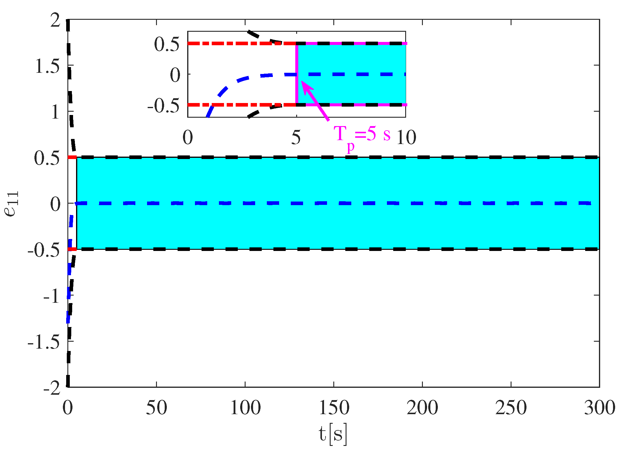
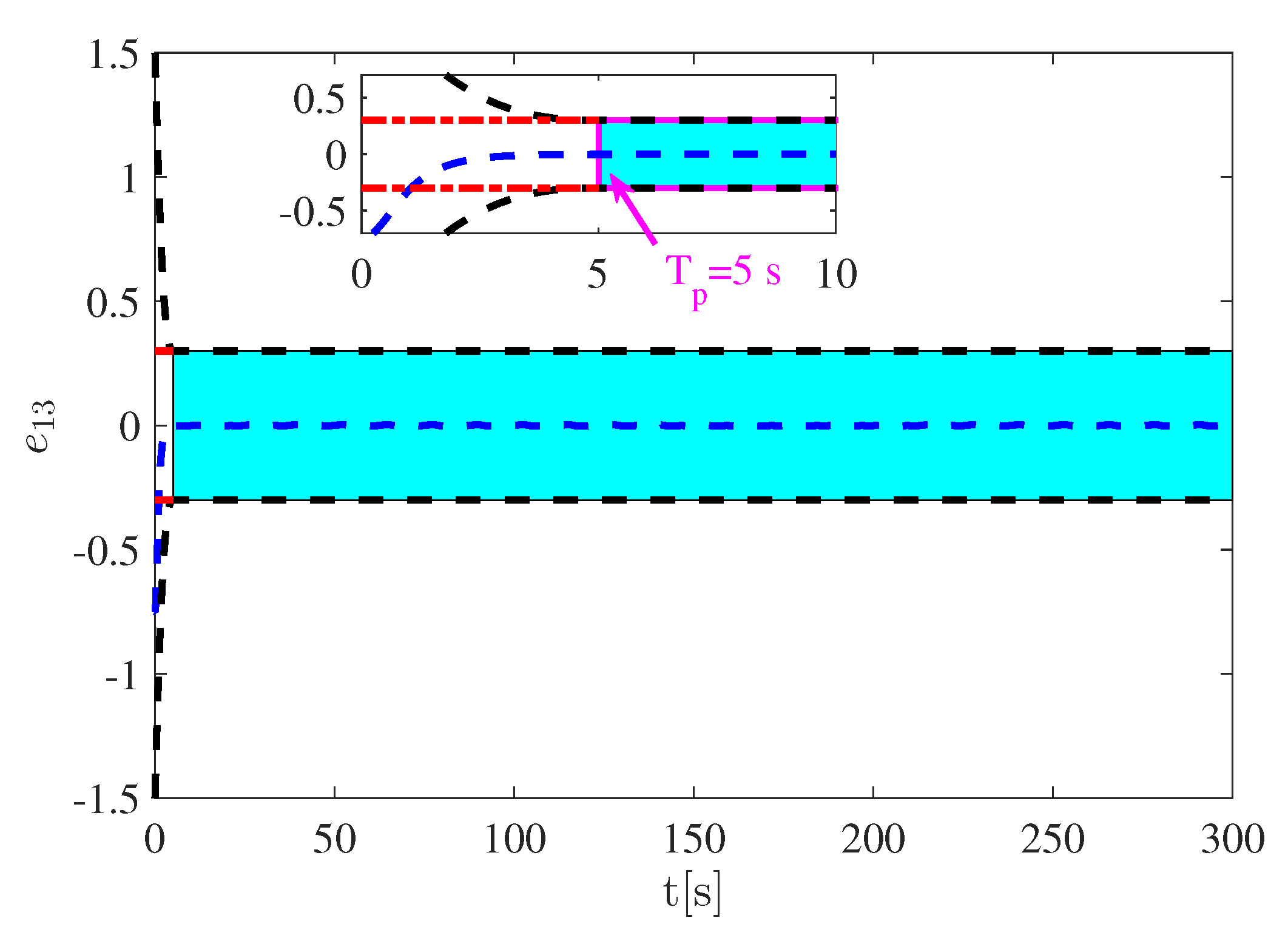
The stability analysis of the controlled system (1) under the designed adaptive SMC law (33)–(36) is given now.
Theorem 1. 
Let Assumptions 1 and 2 hold and the initial condition of the tracking error satisfy (24). Consider the USV (1) subject to actuator faults, dead zones and input quantization. If the adaptive SMC scheme is selected as (33)–(35) and the control gain is selected as (36) with the sliding variable given in (29), then the tracking error e 1 and the sliding variable s converge to predefined bounds | e 1 j | < φ j and | s j | < ε j within a predefined-time, respectively. In addition, the variable σ j always remains in the predefined region | σ j | < ε j and the unconstrained transformation error θ j is asymptotically bounded by ε j c 1 for j = 1 , 2 , 3 .
Proof. 
By substituting (33)–(35) into (32), we have
σ ˙ = h k sgn ( σ ) ,
where h = Γ R M 1 ( f 2 + ( κ ρ 1 ) u ) are the lumped uncertainties. Based on Assumption 1, a state-dependent upper bound structure can be established for the unknown term h as follows
h l 3 + l 4 ξ + l 5 ξ 2 ,
where l 3 > 0 , l 4 > 0 , l 5 > 0 are unknown optimal values and ξ is given in (16). In the light of (36) and (38), the upper bound of the unknown term h holds
σ l j = ε j l 3 + l 4 ξ + l 5 ξ 2 l 3 + l 4 ξ + l 5 ξ 2 + a j ,
and it follows that 0 < σ l j < ε j .
From (30) and (31), we have σ j ( 0 ) = 0 < σ l j . According to (36) and (37), the variable σ j cannot remain at zero. That is, | σ j | starts to increase. Considering (38) and (39), if the variable σ j is located in the domain | σ j ( t ) | σ l j , then | σ j | continues to increase. Now consider that variable σ j has moved into region σ l j < | σ j ( t ) | < ε j . The following hypothesis is given: the variable σ j will converge to the region | σ j ( t ) | σ l j again within a finite time. In summary, the variable σ j remains inside | σ j ( t ) |   <   ε j for t 0 .
To confirm the above hypothesis, we consider that the variable σ j has moved into the region | σ j ( t ) | > σ l j from the initial state. Choose the following Lyapunov function
V 1 = j = 1 3 V 1 j = j = 1 3 1 2 σ j 2 + 1 2 k j 2 ( t , σ j ( t ) ) .
The first derivative of V 1 j is described as follows
V ˙ 1 j = σ j σ ˙ j + k j ( t , σ j ( t ) ) k ˙ j ( t , σ j ( t ) ) .
Note that k ˙ j ( t , σ j ( t ) ) in (41) can be expressed as
k ˙ j ( t , σ j ( t ) ) = k j t , σ j t σ j t σ j t t .
Considering (36) and the properties of the barrier function described in Remark 4, the following two cases need to be discussed.
Case I: σ l j < σ j < ε j . Taking into account (36), (38) and the scalar form of (37), we have
k j t , σ j t σ j t σ j t t = a j ε j ε j σ j t 2 h j k j t , σ j t a j ε j ε j σ j t 2 l 3 + l 4 ξ + l 5 ξ 2 k j t , σ j t .
Case II: ε j < σ j < σ l j . Similarly, the following inequality holds
k j t , σ j t σ j t σ j t t = a j ε j ε j | σ j t | 2 h j + k j t , σ j t a j ε j ε j | σ j t | 2 l 3 + l 4 ξ + l 5 ξ 2 k j t , σ j t .
Substituting (37), (43) and (44) into (41) yields
V ˙ 1 j σ j ( h j k j sgn ( σ j ) ) + k j ( t , σ j ( t ) ) a j ε j ε j | σ j t | 2 l 3 + l 4 ξ + l 5 ξ 2 k j t , σ j t | σ j | k j ( t , σ j ( t ) ) ( l 3 + l 4 ξ + l 5 ξ 2 ) k j ( t , σ j ( t ) ) a j ε j ε j | σ j t | 2 k j ( t , σ j ( t ) ) ( l 3 + l 4 ξ + l 5 ξ 2 ) = Ξ j | σ j | χ j Ξ j k j ( t , σ j ( t ) ) ,
where Ξ j = k j t , σ j t ( l 3 + l 4 ξ + l 5 ξ 2 ) and χ j = a j ε j ε j σ j 2 .
In view of σ l j < | σ j ( t ) | < ε j and (36), we get
k j ( t , σ j ( t ) ) > k j ( σ l j ) = l 3 + l 4 ξ + l 5 ξ 2 ,
which leads to Ξ j > 0 and χ j > 0 .
Then, V ˙ 1 j can be described as
V ˙ 1 j Ξ j | σ j | χ j Ξ j k j ( t , σ j ( t ) ) = Ξ j 2 ( | σ j | 2 + χ j k j ( t , σ j ( t ) ) 2 ) Ξ j 2 min { 1 , χ j } ( | σ j | 2 + k j ( t , σ j ( t ) ) 2 ) Ξ j 2 min { 1 , χ j } V 1 j 1 / 2 .
It follows that the variable σ j converges to the region | σ j |     σ l j in a finite time. Thus, we can conclude that the variable σ j remains within the region | σ j |   <   ε j for t 0 . Moreover, according to the definition of the auxiliary function, σ j = s j when t T s . Therefore, one can further deduce that the sliding variable s j converges to the region | s j |   <   ε j at the predefined time T s .
On the basis of the above analysis, the following conclusions can be made further. According to Lemma 1 with n = 2 , the transformation error θ j is asymptotically bounded by
| θ j |     | s j | c 1 < ε j c 1 , j = 1 , 2 , 3
It follows that the transformation error θ is bounded. Note that G ( θ j ) is a strictly increasing function satisfying lim θ j G θ j = α j and lim θ j G θ j = β j . Thus, z j α j , β j and α j φ j ( t ) < e 1 j ( t ) < β j φ j ( t ) hold. In other words, the tracking error e 1 j satisfies the inequality condition (24) for t > 0 and converges within the bound | e 1 j |   <   φ j within a predefined time ( j = 1 , 2 , 3 ) . In addition, according to Definition 2, the solution of the tracking error system (20) is practically predefined-time stable. □
Remark 6. 
As shown in (37) and (38), the mixed effects of input quantization, actuator faults and dead zones are treated as uncertainties and handled by the adaptive control gain k.
Remark 7. 
For the sake of simplicity of design, this paper uses a linear sliding surface as shown in (29). In application, it can be further extended to other types of sliding surface according to the control objective, such as integral sliding surfaces and non-singular terminal sliding surfaces.
Remark 8. 
Note that the quadratic Lyapunov function given in (40) is used to analyze the system stability. To achieve a better tracking performance, non-quadratic Lyapunov functions can be further considered. In [46,47], it is expounded how to achieve an excellent tracking performance by tuning the parameter α in the Lyapunov function. In particular, the quadratic Lyapunov function V 1 can be regarded as a special form when α = 1 .

4. Simulations

In this section, numerical simulations based on CyberShip II [1] are conducted to verify the effectiveness of the designed controller. CyberShip II is a 1:70 scale replica of a supply ship. The ship has a length of 1.225 m and a breadth of 0.29 m. Furthermore, it is fully driven by two main propellers, one bow thruster and two aft rudders. The main parameters of CyberShip II are given in Table 1.
In the simulation, the initial conditions of the model ship are designated as η ( 0 ) = [ 1.3 1.6 0.75 ] T and ν ( 0 ) = [ 0 0 0 ] T . The desired trajectory is chosen as η d = [ 2 sin ( 0.2 t + π / 5 ) 1.5 cos ( t π / 6 ) cos ( 0.5 t ) ] T . The unknown parts of the model of the USV are assumed to be Δ C ( ν ) = 1 % C 0 ( ν ) and Δ D ( ν ) = 1 % D 0 ( ν ) . Here, partial loss of effectiveness faults and bias faults are considered simultaneously to verify the robustness of the proposed control method. Note that the USV has had an actuator fault since T f = 20 s. The actuator fault parameter is specified as κ = [ 0.5 0.3 0.3 ] T and the bias fault is selected as τ b = [ 0.8 sin ( t ) 0.5 cos ( t ) 0.8 sin ( t ) + 0.5 cos ( t ) ] T . The actuator dead zone parameters in (10) are selected as ρ = 1.2 , d l = [ 0.5 0.5 0.5 ] T and d r = [ 0.5 0.5 0.5 ] T , respectively. The parameters of the hysteresis quantizer (11) are selected as z m i n = [ 0.1 0.1 0.1 ] T and δ = [ 0.1 0.1 0.1 ] T . The parameters of the performance function (21) are chosen as φ 0 = [ 2 2 1.5 ] T , φ = [ 0.5 0.5 0.3 ] T , T p = 5 s and b = [ 0.6 0.6 0.6 ] T . The parameters of (24) are selected as α = β = [ 1 1 1 ] T . The parameters of the control gain are selected as k ( 0 ) = [ 7 7 1 ] T , a = [ 2 2 2 ] T and ε = [ 0.012 0.012 0.012 ] T . The parameters of the auxiliary function (31) are chosen as T s = 1 s and Q = 2 . To demonstrate the performance of the proposed predefined time adaptive SMC method, a comparison with the state-of-the-art adaptive SMC method [12] is performed.
The actual motion trajectory and desired trajectory of the USV are shown in Figure 2. It can be seen that the USV can track the desired trajectory η d under the designed control method. The tracking performance of the USV in directions x, y and ψ is shown in Figure 3. Further, Figure 4, Figure 5 and Figure 6 exhibit the variation curves of the tracking error of the USV in the x, y and ψ directions, respectively. It can be seen that the tracking error curves are all within the predefined behavior boundary, which verifies that the prescribed performance control on the tracking error is achieved. In addition, the tracking errors all converge to the preset bound φ = [ 0.5 0.5 0.3 ] T within the predefined time T p = 5 s.
The behavior of the sliding variables for the proposed method and the method in [12] is shown in Figure 7. It is observed from Figure 7 that under the proposed method, the sliding variable converges to the preset bound ε = [ 0.012 0.012 0.012 ] T within the predefined time T s = 1 s and does not escape for t T s . On the other hand, when the actuator fault occurs at T f = 20 s, the method in [12] cannot guarantee that the sliding variable remains within the previous ultimate bound. In contrast, the ultimate bound of the sliding variable under the proposed method is independent of the upper bound of the lumped uncertainty. Thus, the sliding variable will not leave the predefined bound even if the actuator fault occurs. It should be noted that the selection of the time constant T s and the predefined bound ε is a trade-off between the actual situation and the control objective. The smaller the value selected, the larger the control torque will be, which is unrealistic. The variation curves of the adaptive control gain are shown in Figure 8. From (37), the effect of the actuator fault is treated as a disturbance and handled by the control gain. This is why the control gain increases for a short time after T f = 20 s. Figure 9 shows the designed control signal u and quantized signal q ( u ) . The quantization effect of the hysteresis quantizer can be clearly seen from the partially zoomed-in area. Figure 10 depicts the actual control signals under the proposed method and the method in [12]. It can be seen from Figure 10 that compared with the method in [12], the proposed method effectively reduces chattering in SMC. The reason is that the control signal generated by the proposed method is continuous, exactly as mentioned in Remark 4.

5. Conclusions

In this paper, the trajectory tracking SMC problem of a USV subject to system uncertainties, external disturbances, input quantization, actuator faults and dead zones is studied. A hysteresis quantizer is used to relax the transmission bandwidth requirements from the controller to the actuator while avoiding chattering in the quantized signal. The introduction of an auxiliary function facilitates the design of an adaptive SMC method based on a barrier function. Under the designed controller, the boundedness of both the unconstrained transformation error θ and the variable σ is guaranteed. Then, it is concluded that the predefined transient and steady-state tracking performance is achieved and the tracking error can converge to the user-defined bound within a predefined time. In addition, the sliding variable can converge to the user-defined bound within a predefined time due to the introduction of an auxiliary function. The simulation results demonstrate the effectiveness of the developed control scheme.

Author Contributions

Conceptualization, T.J. and Y.Y.; methodology, T.J. and Y.Y.; software, T.J.; validation, T.J.; formal analysis, T.J.; investigation, T.J.; resources, T.J., Y.Y. and S.-H.Y.; data curation, T.J.; writing—original draft preparation, T.J.; writing—review and editing, T.J. and Y.Y.; visualization, T.J.; supervision, Y.Y.; project administration, Y.Y.; funding acquisition, Y.Y. and S.-H.Y. All authors have read and agreed to the published version of the manuscript.

Funding

This work was supported in part by the Natural Science Foundation of China under grants 62173054 and 62073054 and in part by the Natural Science Foundation of Liaoning under grant 2021-MS-142.

Institutional Review Board Statement

Not applicable.

Informed Consent Statement

Not applicable.

Data Availability Statement

The datasets generated during and/or analyzed during the current study are available from the corresponding author on reasonable request.

Conflicts of Interest

The authors declare no conflict of interest.

References

  1. Skjetne, R.; Smogeli, Ø.; Fossen, T. Modeling, identification, and adaptive maneuvering of Cybership II: A complete design with experiments. IFAC Proc. 2004, 37, 203–208. [Google Scholar] [CrossRef]
  2. Wu, D.; Yuan, K.; Huang, Y.; Yuan, Z.; Hua, L. Design and test of an improved active disturbance rejection control system for water sampling unmanned surface vehicle. Ocean. Eng. 2022, 245, 110367. [Google Scholar] [CrossRef]
  3. Shen, H.; Yin, Y.; Qian, X. Fixed-time formation control for unmanned surface vehicles with parametric uncertainties and complex disturbance. J. Mar. Sci. Eng. 2022, 10, 1246. [Google Scholar] [CrossRef]
  4. Wen, G.; Ge, S.; Chen, C.; Tu, F.; Wang, S. Adaptive tracking control of surface vessel using optimized backstepping technique. IEEE Trans. Cybern. 2018, 49, 3420–3431. [Google Scholar] [CrossRef] [PubMed]
  5. Zhang, Q.; Guo, C. Anti-disturbance lyapunov-based model predictive control for trajectory tracking of dynamically positioned ships. J. Mar. Sci. Eng. 2023, 11, 281. [Google Scholar] [CrossRef]
  6. Chen, H.; Tang, G.; Wang, S.; Guo, W.; Huang, H. Adaptive fixed-time backstepping control for three-dimensional trajectory tracking of underactuated autonomous underwater vehicles. Ocean. Eng. 2023, 275, 114109. [Google Scholar] [CrossRef]
  7. Degorre, L.; Delaleau, E.; Chocron, O. A survey on model-based control and guidance principles for autonomous marine vehicles. J. Mar. Sci. Eng. 2023, 11, 430. [Google Scholar] [CrossRef]
  8. Liu, W.; Ye, H.; Yang, X. Super-twisting sliding mode control for the trajectory tracking of underactuated USVs with disturbances. J. Mar. Sci. Eng. 2023, 11, 636. [Google Scholar] [CrossRef]
  9. Yu, X.; Feng, Y.; Man, Z. Terminal sliding mode control—An overview. IEEE Open J. Ind. Electron. 2020, 2, 36–52. [Google Scholar] [CrossRef]
  10. Yan, Y.; Zhao, X.; Yu, S.; Wang, C. Barrier function-based adaptive neural network sliding mode control of autonomous surface vehicles. Ocean. Eng. 2021, 238, 109684. [Google Scholar] [CrossRef]
  11. Wang, D.; Kong, M.; Zhang, G.; Liang, X. Adaptive second-order fast terminal sliding-mode formation control for unmanned surface vehicles. J. Mar. Sci. Eng. 2022, 10, 1782. [Google Scholar] [CrossRef]
  12. Jiang, T.; Yan, Y.; Wu, D.; Yu, S.; Li, T. Neural network based adaptive sliding mode tracking control of autonomous surface vehicles with input quantization and saturation. Ocean. Eng. 2022, 265, 112505. [Google Scholar] [CrossRef]
  13. Qiao, L.; Zhang, W. Trajectory tracking control of AUVs via adaptive fast nonsingular integral terminal sliding mode control. IEEE Trans. Industr. Inform. 2019, 16, 1248–1258. [Google Scholar] [CrossRef]
  14. Chao, L.; Ma, H.; Tian, S.; Li, Y. Adaptive barrier sliding-mode control considering state-dependent uncertainty. IEEE Trans. Circuits Syst. II Express Briefs. 2021, 68, 3301–3305. [Google Scholar] [CrossRef]
  15. Guo, G.; Zhang, P. Asymptotic stabilization of USVs with actuator dead-zones and yaw constraints based on fixed-time disturbance observer. IEEE Trans. Veh. 2020, 69, 302–316. [Google Scholar] [CrossRef]
  16. Wang, N.; Zhu, Z.; Qin, H.; Deng, Z.; Sun, Y. Finite-time extended state observer-based exact tracking control of an unmanned surface vehicle. Int. J. Robust Nonlinear Control. 2021, 31, 1704–1719. [Google Scholar] [CrossRef]
  17. Zhang, J.; Yu, S.; Yan, Y. Fixed-time velocity-free sliding mode tracking control for marine surface vessels with uncertainties and unknown actuator faults. Ocean. Eng. 2020, 201, 107107. [Google Scholar] [CrossRef]
  18. Chang, L.; Han, Q.; Ge, X.; Zhang, C.; Zhang, X. On designing distributed prescribed finite-time observers for strict-feedback nonlinear systems. IEEE Trans. Cybern. 2019, 51, 4695–4706. [Google Scholar] [CrossRef]
  19. Jiménez-Rodríguez, E.; Muñoz-Vázquez, A.; Sánchez-Torres, J.; Defoort, M.; Loukianov, A. A Lyapunov-like characterization of predefined-time stability. IEEE Trans. Autom. Control. 2020, 65, 4922–4927. [Google Scholar] [CrossRef] [Green Version]
  20. Liang, C.; Ge, M.; Liu, Z.; Ling, G.; Liu, F. Predefined-time formation tracking control of networked marine surface vehicles. Control Eng. Pract. 2020, 107, 104682. [Google Scholar] [CrossRef]
  21. Shao, K.; Zheng, J.; Wang, H.; Man, Z. Terminal time regulator-based exact-time sliding mode control for uncertain nonlinear systems. Int. J. Robust Nonlinear Control. 2022, 32, 7536–7553. [Google Scholar] [CrossRef]
  22. Ma, H.; Liu, W.; Xiong, Z.; Li, Y.; Liu, Z.; Sun, Y. Predefined-time barrier function adaptive sliding-mode control and its application to piezoelectric actuators. IEEE Trans. Industr. Inform. 2022, 18, 8682–8691. [Google Scholar] [CrossRef]
  23. Souissi, S.; Boukattaya, M. Time-varying nonsingular terminal sliding mode control of autonomous surface vehicle with predefined convergence time. Ocean. Eng. 2022, 263, 112264. [Google Scholar] [CrossRef]
  24. Wu, Z.; Ni, J.; Qian, W.; Bu, X.; Liu, B. Composite prescribed performance control of small unmanned aerial vehicles using modified nonlinear disturbance observer. ISA Trans. 2021, 116, 30–45. [Google Scholar] [CrossRef]
  25. Zhu, G.; Ma, Y.; Li, Z.; Malekian, R.; Sotelo, M. Adaptive neural output feedback control for MSVs with predefined performance. IEEE Trans. Veh. Technol. 2021, 70, 2994–3006. [Google Scholar] [CrossRef]
  26. Zhao, J.; Cai, C.; Liu, Y. Barrier lyapunov function-based adaptive prescribed-time extended state observers design for unmanned surface vehicles subject to unknown disturbances. Ocean. Eng. 2023, 270, 113671. [Google Scholar] [CrossRef]
  27. Wang, Y.; Hao, L.; Li, T.; Chen, C. Integral sliding mode-based fault-tolerant control for dynamic positioning of unmanned marine vehicles based on a T-S fuzzy model. J. Mar. Sci. Eng. 2023, 11, 370. [Google Scholar] [CrossRef]
  28. Yao, Q. Adaptive finite-time sliding mode control design for finite-time fault-tolerant trajectory tracking of marine vehicles with input saturation. J. Frank. Inst. 2020, 357, 13593–13619. [Google Scholar] [CrossRef]
  29. Li, Y.; He, J.; Zhang, Q.; Zhang, W.; Li, Y. Predefined-time fault-tolerant trajectory tracking control for autonomous underwater vehicles considering actuator saturation. Actuators 2023, 12, 171. [Google Scholar] [CrossRef]
  30. Hao, L.; Zhang, Y.; Li, H. Fault-tolerant control via integral sliding mode output feedback for unmanned marine vehicles. Appl. Math. Comput. 2021, 401, 126078. [Google Scholar] [CrossRef]
  31. Ma, M.; Wang, T.; Guo, R.; Qiu, J. Neural network-based tracking control of autonomous marine vehicles with unknown actuator dead-zone. Int. J. Robust Nonlinear Control. 2021, 32, 2969–2982. [Google Scholar] [CrossRef]
  32. Cui, R.; Zhang, X.; Cui, D. Adaptive sliding-mode attitude control for autonomous underwater vehicles with input nonlinearities. Ocean. Eng. 2016, 123, 45–54. [Google Scholar] [CrossRef]
  33. Zhang, P.; Guo, G. Fixed-time switching control of underactuated surface vessels with dead-zones: Global exponential stabilization. J. Frank. Inst. 2019, 357, 11217–11241. [Google Scholar] [CrossRef]
  34. Zhang, G.; Yao, M.; Zhang, W.; Zhang, W. Improved composite adaptive fault-tolerant control for dynamic positioning vehicle subject to the dead-zone nonlinearity. IET Control. Theory Appl. 2021, 15, 2067–2080. [Google Scholar] [CrossRef]
  35. Yan, Y.; Yu, S. Sliding mode tracking control of autonomous underwater vehicles with the effect of quantization. Ocean. Eng. 2018, 151, 322–328. [Google Scholar] [CrossRef]
  36. Hao, L.; Zhang, H.; Li, H.; Li, T. Sliding mode fault-tolerant control for unmanned marine vehicles with signal quantization and time-delay. Ocean. Eng. 2020, 215, 107882. [Google Scholar] [CrossRef]
  37. Yan, Y.; Yu, S.; Yu, X. Quantized super-twisting algorithm based sliding mode control. Automatica 2019, 105, 43–48. [Google Scholar] [CrossRef]
  38. Hao, L.; Zhang, H.; Guo, G.; Li, H. Quantized sliding mode control of unmanned marine vehicles: Various thruster faults tolerated with a unified model. IEEE Trans. Syst. Man Cybern. Syst. 2019, 51, 2012–2026. [Google Scholar] [CrossRef]
  39. Shao, X.; Shi, Y. Fault-tolerant quantized control for flexible air-breathing hypersonic vehicles with appointed-time tracking performances. IEEE Trans. Aerosp Electron. Syst. 2021, 57, 1261–1273. [Google Scholar] [CrossRef]
  40. Li, A.; Liu, M.; Cao, X.; Liu, R. Adaptive quantized sliding mode attitude tracking control for flexible spacecraft with input dead-zone via Takagi-Sugeno fuzzy approach. Inf. Sci. 2021, 587, 746–773. [Google Scholar] [CrossRef]
  41. Zhang, T.; Bai, R.; Li, Y. Practically predefined-time adaptive fuzzy quantized control for nonlinear stochastic systems with actuator dead zone. IEEE Trans. Fuzzy Syst. 2022, 31, 1240–1253. [Google Scholar] [CrossRef]
  42. Zhao, Z.; Zhang, J.; Liu, Z.; He, W.; Hong, K. Adaptive quantized fault-tolerant control of a 2-DOF helicopter system with actuator fault and unknown dead zone. Automatica 2023, 148, 110792. [Google Scholar] [CrossRef]
  43. Shao, K.; Zheng, J. Predefined-time sliding mode control with prescribed convergent region. IEEE-CAA J. Autom. Sin. 2022, 9, 934–936. [Google Scholar] [CrossRef]
  44. Slotine, J.; Li, W. Applied Nonlinear Control; Englewood Cliffs: Prentice Hall, NJ, USA, 1991; pp. 278–280. [Google Scholar]
  45. Yin, Z.; Suleman, A.; Luo, J.; Wei, C. Appointed-time prescribed performance attitude tracking control via double performance functions. Aerosp. Sci. Technol. 2019, 93, 105337. [Google Scholar] [CrossRef]
  46. Tao, G. Model reference adaptive control with L1+α tracking. Int. J. Control. 1996, 64, 859–870. [Google Scholar] [CrossRef]
  47. Hosseinzadeh, M.; Yazdanpanah, M. Performance enhanced model reference adaptive control through switching non-quadratic Lyapunov functions. Syst. Control. Lett. 2015, 76, 47–55. [Google Scholar] [CrossRef]
Figure 1. The structure diagram of the controlled system.
Jmse 11 01244 g001
Figure 2. The desired trajectory and actual trajectory of the USV.
Jmse 11 01244 g002
Figure 3. Position and heading.
Jmse 11 01244 g003
Figure 4. Tracking error of position x.
Jmse 11 01244 g004
Figure 5. Tracking error of position y.
Jmse 11 01244 g005
Figure 6. Tracking error of heading ψ .
Jmse 11 01244 g006
Figure 7. Sliding variable s [12].
Jmse 11 01244 g007
Figure 8. Adaptive control gain k.
Jmse 11 01244 g008
Figure 9. The control signal u and the quantized signal q ( u ) .
Jmse 11 01244 g009
Figure 10. Actual control input τ [12].
Jmse 11 01244 g010
Table 1. Main parameters of CyberShip II.
m = 23.8 I z = 1.76 x g = 0.046 X u = 0.07225
X | u | u = 1.3274 X u u u = 5.8664 Y ν = 0.8896 Y | ν | ν = 36.4728
Y | r | ν = 0.805 Y | ν | r = 0.845 Y | r | r = 3.45 N | r | r = 0.75
Y r = 7.25 N ν = 0.0313 N | ν | ν = 3.9564 X u ˙ = 2
Y ν ˙ = 10 Y r ˙ = 0 N ν ˙ = 0 N r ˙ = 1
N | r | ν = 0.13 N r = 1.9 N | ν | r = 0.08
Disclaimer/Publisher’s Note: The statements, opinions and data contained in all publications are solely those of the individual author(s) and contributor(s) and not of MDPI and/or the editor(s). MDPI and/or the editor(s) disclaim responsibility for any injury to people or property resulting from any ideas, methods, instructions or products referred to in the content.

