Numerical Investigation of Self-Propulsion Performance and Noise Level of DARPA Suboff Model

Abstract

Propulsion noise is an enduring problem of significant military and environmental importance. Hence, it is crucial to investigate propeller noise characteristics. In this study, the hydrodynamic performance and noise level of the DARPA (Defense Advanced Research Projects Agency) Suboff submarine with the E1619 propeller were analyzed. The hull resistance and propeller hydrodynamics were studied separately, and the numerical results were validated using available experimental values. The self-propulsion point was determined by matching the hull resistance and propeller thrust following ITTC (International Towing Tank Conference) convention. Based on hydrodynamics and acoustic Ffowcs Williams–Hawkings (FW–H) models, the underwater-radiated noise characteristics in the self-propulsion state were simulated. The calculations indicated that the contribution of the quadrupole term in the FW–H equation is not negligible in the high-frequency band. Compared with the noise of open-water propellers, the spectrum of the E1619 propeller in its self-propulsion state is more complex, and the upstream noise is amplified.

1. Introduction

The shipping industry has rapidly developed in the past several decades. Consequently, noise pollution associated with ship operations, which has a negative impact on human and marine animal habitats and damages local ecologies, has attracted much attention. Moreover, noise characteristics have been an important technical index based on the specific tasks and operational requirements of ships. As one of the biggest noise sources, propeller noise is a signal that can be tracked by sonar. Consequently, the sound-pressure level is a limiting factor of ship survival. Thus, there are clear military and environmental imperatives associated with ship noise reduction.

In a solid structure, the main mechanisms of sound generation can be classified as follows: vortex shedding noise, turbulent structure interaction noise, and trailing edge noise (Roger [1]). Vortex shedding noise is generated from a vortex released from blunt body in fluid. The time-varying cycle on the body, caused by vortex shedding, generates a pulsating power on the body itself, which is transmitted to the fluid and propagated as sound. The turbulence structure interaction noise comes from the local pressure pulsation generated by the vortex structure colliding on the solid surface on the body surface feeding into the remote acoustic field. Trailing edge noise is generated due to the interaction between boundary-layer instability and surface edge, which is very important for all rotating blade technologies. Numerous experimental and numerical studies have been conducted concerning underwater-radiated noise. Presently, many hydrodynamic and acoustic studies have focused on ship propellers at different flows. These accumulated empirical data have contributed to better understanding the principles of noise generation and propagation.

Jessup [2] and Chesnakas and Jessup [3] analyzed the complex three-dimensional flow around a propeller using a laser Doppler velocimeter. Recent studies have provided detailed descriptions of tip vortex evolution and interactions with hub vortices under different operating conditions. Felli et al. [4] conducted a noise-source analysis on a rudder behind the marine propeller. To separate the acoustic and hydrodynamic components of the recorded pressure signal, a novel wavelet-based filtering program was proposed. It was found that acoustic disturbances were mainly related to the unsteady load variation in the rudder and shear layer fluctuation of the propeller flow tube.

Computational fluid dynamics (CFD) can be applied to the numerical prediction of propeller underwater noise in two steps. The first involves analyzing the flow around the propeller, followed by acoustic computations. Presently, many empirical and semi-empirical calculation methods are used. In 1952, Lighthill [5] established the theoretical background, which is usually used in the study of aerodynamic noise. Lighthill first introduced the concept of aeroacoustic analogy, including the use of equivalent noise-source systems to replace the actual flow field responsible for generating noise. The noise source acts on the unified stagnation flow controlled by the standard sound propagation equation. Then, the aerodynamic characteristics of the source become the main problem in noise prediction. In 1955, Curle [6] further extended the concept proposed by Lighthill, including the influence of fluid interaction on sound. In 1969, Ffowcs Williams and Hawkings [7] further extended the analogy proposed by Curle to take any surface motion into account. The Ffowcs Williams–Hawking (FW–H) methods provide a milestone of acoustic prediction of underwater noise level. The FW–H equation has been widely used in the numerical prediction of underwater noise of marine propellers. Seol, Suh and Lee [8] used the boundary element method with FW–H equations to understand the non-cavitating noise produced by propellers. They resolved the flow field around the propeller and predicted its far-field acoustic characteristics. Salvatore and Ianniello [9] divided the sound pressure of noise into thickness and load terms and showed that FW–H noise predictions were consistent with those of the Bernoulli equation. Seol, Suh and Lee [10] further studied far-field noise radiation by combining a thin-plate cavity model with the FW–H equation. Cianferra et al. [11] combined FW–H and large-eddy simulations (LES) to study the influence of a simple blunt-body shape on radiated noise. Cianferra et al. [12] subsequently evaluated the noise characteristics of a finite cylinder using the same combination of FW–H and LES. Their study showed that the quadrupole term affected a wide frequency range. According to their results, the quadrupole term generated by the cube was far less relevant than that generated by a slender square cylinder, and this difference was caused by wake persistence. The influence of free surface has also received attention from scholars. Efremov and Milanov [13] and Ling et al. [14] studied the performance of a standard model “DARPA Suboff” submarine at shallowly immersion conditions. The attenuation characteristics of the effect of free surface distance on performance were described in the study.

From this literature review, it is clear that the noise of open-water propellers has been well studied. Here, we examine the combined radiated noise of the hull and propeller under self-propulsion and their hydrodynamic interference. Our calculation model leverages the Suboff AFF8 submarine model and related E1619 propeller model. First, a numerical simulation of the hydrodynamic performance of the hull and the open-water propeller is carried out. Then, the hull and propeller are combined to simulate a self-propulsion submarine. The CFD results are compared with literature data to ensure the reliability of flow calculations. Finally, the underwater noise of the open-water propeller and that of the self-propulsion propeller are separately predicted. The diversity of acoustic characteristics between open-water and self-propulsion is then discussed.

2. Numerical Model

The Reynolds-averaged Navier–Stokes (RANS) numerical model is introduced first. Subsequently, the FW–H underwater acoustic model is introduced with corresponding methodology and analysis.

2.1. RANS Equation

RANS equations are used to model the flow around a hull and propeller. Commercial CFD software STAR-CCM+ (v. 14.02, Siemens PLM Software, Plano, TX, USA) is used to solve viscosity problems for numerical simulation. Turbulence models provide closure relations for the RANS equations, which govern the transport of the mean-flow quantities. The mean mass and momentum transport equations used by STAR-CCM+ can be expressed as

$$\frac{\partial \rho }{\partial t}+\nabla \cdot (\rho \overline{v})=0$$

(1)

$$\frac{\partial }{\partial t}(\rho \overline{v})+\nabla \cdot (\rho \overline{v}\otimes \overline{v})=-\nabla \cdot \overline{p}I+\nabla \cdot (T+T_t)+f_b$$

(2)

where $\rho$ is the density, $\overline{v}$ and $\overline{p}$ are respectively the mean velocity and pressure, $I$ is the identity tensor, $T$ is the viscous stress tensor, $T_t$ is the Reynolds stress tensor, and $f_b$ is the resultant of the body forces (e.g., gravitational and centrifugal). These equations are nearly identical to the original Navier–Stokes equations, except for the Reynolds stress tensor, which appears in the momentum transport equation.

The unsteady flow field is calculated using the RANS equation. The finite volume method is used to discretize the control equations. The segregated flow model solves the equation in a segregated manner, and the second-order upwind scheme is used to discretise the convection term. The diffusion term is a central difference scheme having a second-order accuracy. The pressure-coupling equations are solved using the semi-implicit method for pressure-linked equations. The first-order scheme is used to calculate the unsteady momentum equation, whereas the second-order scheme is used for noise. The shear stress transport (SST) k–ω turbulence model is adopted to enable more accurate calculation of the flow around the model propeller (Zhu et al. [15]).

2.2. FW–H Equation

The FW–H equation, a non-uniform wave equation derived from the conservation of mass and momentum, is used to predict radiated noise. According to Lighthill’s acoustic analogy (Lighthill [5]), the noise around a rotor and propeller and their different geometries can be predicted using a discrete FW–H equation. The sound pressure can be calculated from a specific surface representing the noise source. There are many methods of solving surface and volume integrals in the FW–H equation. Brentner and Farrassat [16] proposed a solution using simplified functions. The total sound pressure can thus be expressed as

$$p^{\prime }={p^{\prime }}_{\mathrm{T}}+{p^{\prime }}_{\mathrm{L}}$$

(3)

Here, ${p^{\prime }}_{\mathrm{T}}$ is the thickness surface term, and ${p^{\prime }}_{\mathrm{L}}$ is the load surface term, which can be calculated as follows:

$$4\pi {p^{\prime }}_{\mathrm{T}}(x,t)={\displaystyle {\int }_{f=0}{[\frac{{\rho }_0{\dot{v}}_n}{r{(1-M_r)}^2}]}_{\mathrm{ret}}\mathrm{d}s}+{\displaystyle {\int }_{f=0}{[\frac{{\rho }_0{v}_n(r{\dot{M}}_i{r}_i+c_0{M}_r-c_0{M}^2)}{r^2{(1-M_r)}^3}]}_{\mathrm{ret}}\mathrm{d}s}$$

(4)

$$\begin{array}{lll}4\pi {p^{\prime }}_{\mathrm{L}}(x,t)& =& \frac{1}{c_0}{\displaystyle {\int }_{f=0}{[\frac{{\dot{l}}_i{\stackrel{⌢}{r}}_i}{r{(1-M_r)}^2}]}_{\mathrm{ret}}\mathrm{d}s}\\ & & +\frac{1}{c_0}{\displaystyle {\int }_{f=0}{[\frac{l_r(r{\dot{M}}_i{r}_i+c_0{M}_r-c_0{M}^2)}{r^2{(1-M_r)}^3}]}_{\mathrm{ret}}\mathrm{d}s}\\ & & +\frac{1}{c_0}{\displaystyle {\int }_{f=0}{[\frac{l_r-l_i{M}_i}{r^2(1-M_r)}]}_{\mathrm{ret}}\mathrm{d}s}\end{array}$$

(5)

Equations (4) and (5) indicate the solution of the surface integrals for thickness and loading noise terms of the FW–H equation. Here, r is the distance to the receiver, M_r is Mach number in the radiation direction of the receiver, v_i is the flow velocity and l_i is the surface area in the i direction. Further, c₀ is the sound speed, and ρ₀ is the density. The symbol [·] represents derivatives obtained with respect to the retarded time.

2.3. Numerical Calculation of Noise

The general steps of noise calculation are as follows:

(1) The unsteady flow around propeller is solved using the numerical model introduced in Section 2.1.

(2) FW–H is used for post-processing the RANS calculation data. The FW–H acoustic module is applied by setting the relevant parameters and distributing the source-monitoring points (i.e., hydrophones). Then, calculations are performed.

(3) The sound-pressure data of hydrophones are extracted, and the sound-pressure level is determined. Then, a Fourier transform is performed to convert the time-domain signal into one of the frequency domain. The sound-pressure spectrum level is measured in the Hz bandwidth, and the frequency resolution is 1 Hz.

$$L_1=10\lg \left(\frac{p^2\left(f\right)}{p_0^2}\right)=20\lg \left(\frac{p\left(f\right)}{p_0}\right)$$

(6)

where p₀ is the reference sound pressure: 10⁻⁶ Pa.

(4) The third octave band level is calculated according to the noise frequency domain value, and the total sound pressure is calculated.

The third octave spectrum level is the sound-pressure spectrum level of noise at every third octave. Its center frequency, f₀, is (1.01.251.62.02.53.154.05.06.38.0) × 10^M Hz, as annotated by the International Standards Organization. The third octave spectrum level calculated from the sound-pressure spectrum level is

$$L_{1/3oct}=10\lg {\displaystyle \sum _f{10}^{L_1(f)/10}}-10\lg f_0+6.38$$

(7)

where $2^{-\frac{1}{6}}\le f\le 2^{\frac{1}{6}}{f}_0$.

The frequency-band level refers to the sound-pressure level in a certain frequency band. The third octave band level can be calculated from the sound-pressure level to characterize the noise level in a certain frequency band. The expression is

$$L_{band}=10\lg {\displaystyle \sum _{f_1}^{f_h}{10}^{L_1(f)/10}}=10\lg {\displaystyle \sum _{f_i}^{f_h}{f}_i{10}^{L_{1/3oct}(f_i)/10}}-6.38$$

(8)

where f_i represents the center frequency of the third octave in the specified frequency range, and f₁ and f_h are the upper and lower frequency ranges, respectively.

The total sound level refers to the sound-pressure level of the entire frequency band, used to represent the noise level across the entire band (Qian [17]). Its expression is

$$BSL=10\lg {\displaystyle \sum _{f_1}^{f_h}{10}^{L_{band}/10}}$$

(9)

where f₁ and f_h are the upper and lower frequencies, respectively.

3. Hydrodynamic Calculation and Verification

Screw propellers are widely used for submarine propulsion. In this section, the open-water performance of an E1619 propeller and the Suboff resistance are computed using CFD and verified. A self-propulsion simulation of the submarine is then conducted.

3.1. Geometric Models and Parameters

The DARPA Suboff AFF8 is a generic submarine model having a length of 4.36 m and a cylindrical cross section with a maximum diameter of 0.508 m. The main geometric parameters are shown in

Table 1. Main parameters of the DARPA Suboff AFF8 model.

Particular	Symbol	Parameters
Scale ratio	λ	24
Length overall	LOA (m)	4.356
Length between perpendiculars	LBP (m)	4.261
Maximum hull radius	Dmax (m)	0.508
Wetted surface	S (m2)	6.348
Volume of displacement	∇ (m3)	0.706

(Chang et al. [18]).

The E1619 propeller is a seven-bladed highly skewed propeller. The main parameters are shown in

Table 2. Main parameters of the E1619 propeller model.

Particulars	Symbol	Open-Water	Self-Propulsion
Propeller Diameter	D (m)	0.485	0.262
Pitch Ratio	P/D	1.15	1.15
Number of Blades	Z	7	7
Hub Diameter Ratio	Dh/D	0.226	0.226
Rotation Direction		Right hand

. For open-water calculation, the diameter of the E1619 propeller is taken as 0.485 m. The E1619 propeller model shown in Figure 1 is applied. For self-propulsion calculation, the E1619 propeller diameter is 0.262 m, and the length of AFF8 model is 4.356 m referring to Sezen’s self-propulsion calculation configuration (Sezen [19]). The DARPA Suboff AFF8 submarine model with its propeller, as shown in Figure 2, is used.

3.2. Hull Resistance Calculation and Verification

3.2.1. Computational Domain

The computational domain is cuboidal. The lengths of the two short sides of the outer domain are specified as 10D_max, and that of long sides is 4L_OA. The inflow boundary is 1L_OA from the foremost edge of the submarine, and the outflow boundary is 2L_OA from its aft. In addition to the inflow and outflow boundaries, the other four edge interfaces are set as symmetrical faces.

The mesh near the hull area is densified in layers. The densified areas include the boundary layer, the foremost edge of the hull, the command tower, rudders and propeller meshes, as shown in Figure 3. The feature lines at the edges and corners of hydrofoils and command tower are encrypted to ensure that the mesh sufficiently fits the hull geometry. There are ~four million eight hundred eighty thousand grid cells. The mesh is topologically efficient without negative volume elements.

3.2.2. Simulation Results

The computed resistances of the AFF8 model and corresponding available test values (Liu and Huang, [20]) in uniform flows are comparatively studied to verify the accuracy of the CFD numerical simulation and to compare the relative error between calculated and available test values. Under same mesh and settings, simulations at different inflow velocities are performed using the SST k–ω turbulence model. Moreover, full y + treatment is adopted with a y + value between 0 and 30 on the walls.

The computed resistances of the AFF8 model under various speeds are shown in

Table 3. Resistances of the DARPA Suboff AFF8 model.

Velocity (m/s)	Test Value (N) (Liu and Huang [20])	Calculation Value (N)	Error (%)
3.051	102.3	93.75	−8.36
3.051(Turbulence Suppression)	102.3	98.479	−3.735
5.144	283.8	289.856	2.13
6.096	389.2	401.648	3.20
7.161	526.6	538.540	2.27
8.231	675.6	690.525	2.22
9.152	821.1	832.806	1.42

. The results fit well. Referring to the data in the table, the error at 5.144 m/s velocity is within 4%, which is sufficiently accurate, but large at 3.051 m/s. This is because the Reynolds number is relatively low (1.29 × 10⁷) owing to the low speed, which causes the turbulence to be inadequate. Based on the SST k−ω turbulence model, low Reynolds-number damping correction is applied to suppress the turbulence, and the error is reduced to within 4%.

3.2.3. Mesh Independence Verification

To analyze the influence of mesh refinement on the AFF8 model, three meshes (i.e., coarse, medium, and fine) are considered, as shown in

Table 4. Calculation results using grids with different refinements at 5.144 m/s.

Description	Number	Calculation (N)	Test Result (N)	Error (%)
Coarse	2,712,883	292.354	283.8	3.01
Medium	4,888,757	289.856	283.8	2.13
Fine	10,633,931	289.46	283.8	1.99

. Using the SST k−ω turbulence model, the resistance values calculated with grids of varying refinements at a fixed speed of 5.144 m/s are provided.

From Table 4, it is seen that the grid is sufficient for an accurate simulation. The resistances corroborate the calculation algorithm, turbulence settings, and calculation accuracy of the mesh. Mesh independence verification also shows that the current model and grid are sufficiently reliable.

3.2.4. Flow-Field Discussion

The computed resistance can be used to show the reliability of the mesh and physical settings. For the study of noise, the macro force cannot explain the problem. The boundary-layer characteristics around the hull and those of the wake field and other flow-field details are considered to obtain the noise characteristics. This forms the focus of this study. This section aims to discuss the detailed characteristics of the hull and compares the test values.

To compare with the data from Sezen et al. [19], the working condition of 2.75 m/s is selected for further simulation verification. The pressure coefficient, C_p, can be obtained as follows:

$$C_P=(P_0-P_{\infty })/(\rho U_{\infty }^2)$$

(10)

where P₀ is the local pressure, P_∞ is the ambient pressure, ρ is the fluid density, and U_∞ is the inflow velocity.

The pressure distribution of the AFF8 model is shown in Figure 4. Here, C_p is the pressure coefficient and x represents the distance. The apex of the fore segment is the origin, and the direction of the endpoint is positive. Here, L represents the submarine length. The influence of appendages on the pressure is clearly and quantitatively reflected.

The results are in good agreement with the test data. They reflect the sudden change in pressure at the command tower and the hull. When the water flows around the command tower and the airfoil, it causes a sudden change in pressure. When the flow reaches an appendage, it initially increases and then decreases. Then, the change reflects a smaller increase and decrease. The smaller pressure jump can be attributed to the streamline geometry of the appendages, which provide a good rectification effect.

In Figure 5, U represents the dimensionless speed in the x-axis. Vx is the velocity component in the x-axis and V is the inflow velocity. U is the ratio of Vx and V. The wake calculation results agree well with the test results as the inflow velocity is 2.75 m/s, as shown in Figure 5. In Figure 5a, the velocity nephogram refers to the V-shaped depression at positions at 0°, 90°, 180° and 270°. Experimental and numerical results clearly reflect the role of appendages. As aforementioned, in this study, the test values refer to those reported by Crook [21] and Chase [22].

3.3. Calculation of Propeller Open-Water Performance

Referring to Figure 6, the calculation domain of the open-water propeller is cylindrical with a diameter of 8D. The inflow boundary is set to 3D in front of the propeller disc and the outflow boundary is set to 4D behind it. To obtain the flow field around the propeller, the propeller is placed in a small cylinder with a diameter of 2D. Thus, the computational domain is divided into two parts: the rotating region that includes the propeller and the static outside region. The interface between static and rotating regions is set for data transmission and communication. The mesh of the rotating and calculation regions near the propeller is densified. The structured grid is used to divide the mesh and the mesh near the propeller area is encrypted layer-by-layer. The total number of grids is about three million. The mesh quality is shown to be topologically efficient without negative volume elements.

To verify the accuracy of the CFD numerical simulation, the open-water performance of the propeller and its test value are studied in a uniform flow field. Subsequently, the relative error between the calculations and the experimental values is analyzed. During calculation, the advance coefficient falls to within 0.1–1.1. The rotation speed of the E1619 propeller is set to 10.71 rps and the advance coefficient is adjusted by changing the inflow speed with the fixed rotation. At 10.71 rps, the Reynolds number is greater than 3 × 10⁵, which is clearly larger than the critical value. This indicates that the propeller model has reached a turbulent state. When the Reynolds number is larger than the critical value, it has little effect on performance. The turbulence model selected in this section is the SST k–ω model.

Because the open-water inflow is steady and uniform, a multiple reference frame algorithm can be used for steady calculation and to save time. The obtained open-water curve is shown in Figure 7. J represents the advance coefficient; K_T0, K_Q0, and η₀ represent the experimental values of thrust coefficient, torque coefficient, and propeller efficiency, respectively; and K_T, K_Q, and η represent their calculated values, respectively.

Figure 7 shows that the prediction accuracy of the propeller open-water performance is reliable. The comparison between test and calculated values shows that the error between the two values is very small (less than 3%) when the advance coefficient is within 0.7. At a high coefficient, the curve of propeller performance is separated from the test-value curve, and the deviation becomes larger. Generally, the error is acceptable under the advance condition of J < 1.0. The experimental data are obtained from the publication by Di Felice et al. [23].

3.4. Self-Propulsion Simulation

Based on previous numerical simulations of a single propeller with a bare hull, this section reports the simulation of the submarine self-propulsion. The towing force at the self-propulsion point of a real submarine is F_D. To find that of a real submarine, a basic similarity principle is used. First, geometric similarity should be ensured in the model test:

$$\frac{L_s}{L_m}=\frac{D_{ps}}{D_{pm}}=\lambda$$

(11)

During the open-water test, it is necessary that the advance coefficient be equal (movement similarity):

$$J_{0s}=J_{0m}$$

(12)

To relate the model and the real submarine self-propulsion systems, the load of the real propeller and the model propeller must be similar (dynamic similarity). Thus, the propeller load coefficient must also agree. Because the underwater test does not have the same Fourier number similarity relationship as does the surface submarine, there is no direct corresponding relationship between the propeller speeds. Thus, K_T/J₀² is used to negate the propeller. F_D can then be obtained by simple derivation. Ignoring scale effects, F_D can be simplified to

$$F_D=\frac{1}{2}\rho V_m^2{S}_{Tm}(C_{Tm}-C_{Ts})$$

(13)

where V_m is the model speed, C_Tm and C_Ts represent the resistance coefficients of the model and the real ship, respectively. Physically, in the model scale, if the propeller model thrust (T_m) overcomes the resistance (R_m − F_D), the self-propulsion point of the full scale is satisfied, which is equivalent to the total resistance (R_S) of the real ship overcome by the thrust (T_BS) of the actual propeller.

When using a deep submergence test system, the effect of surface wave making can be ignored. Thus, the above formula can be rewritten as follows:

$$F_D=\frac{1}{2}\rho V_m^2{S}_{Tm}(C_{fm}-C_{fs}-\Delta C_T)$$

(14)

The statistics of testing show that the difference between C_fs + $\Delta$C_T and C_fm is less than 0.2 × 10⁻³. It is assumed that the small change in propeller load during the model test has little effect on the self-propulsion factor. Thus, the self-propulsion point can be approximated as F_D ≈ 0. Therefore, the arithmetic mean value of the self-propulsion factor under the speed that exceeds the critical Reynolds number can be used as the self-propulsion factor of the model test. For submarines, although this simplified method is not inflexible, it can meet the requirements of engineering prediction. Therefore, this method is commonplace in submarine underwater self-propulsion studies (Zhu et al. [15]).

Referencing the self-propulsion factor solution (ITTC [24]), the mesh-setting of the calculation is basically the same as that of the bare-hull resistance calculation, except that it is applied to the propeller area. To calculate the area division, please refer to the previous description of resistance calculation and Figure 8. For calculation, the thrust identification method is used. According to the values of thrust and torque obtained from the self-propulsion analysis, their coefficients are calculated. To obtain the propulsion coefficient of the submarine self-propulsion approach point, the thrust coefficient is input into the open-water curve, and the corresponding coefficient is obtained. Here, both the open-water curve obtained by experiments and numerical simulation can be used to calculate the propulsion coefficient of the self-propulsion point. In order to compare with the result of Sezen et al. [19], the inflow speed is set to 3.051 m/s. Thus, when the self-propulsion point is reached, the rotation speed, n, of the propeller is 10.20 rps. The output thrust (T) and torque (Q) change periodically over time. Figure 9a,c shows the converging thrust and torque pulsations of a single blade, respectively. After applying the fast Fourier transform (FFT), the relationship between pulsation amplitude and frequency of a single blade is obtained, as shown in Figure 9b,d. After the Fourier transform, there are circumferential components independent of the blade and shaft frequencies as given in Figure 9b,d, which are attributed to the forward hull interference. The presence of appendages leads to the inflow non-uniformity and instability of the propeller.

The dimensionless thrust and torque coefficients of the propeller can be calculated using Equations (15) and (16). Here, T is thrust, Q is torque, D is the propeller diameter, n is the propeller speed and ρ is the water density.

$$Kt=T/\rho n^2{D}^4$$

(15)

$$Kq=Q/\rho n^2{D}^5$$

(16)

The thrust coefficient, K_T, is 0.231, and the torque coefficient, K_Q, is 0.04566. According to ITTC [24], the corresponding self-propulsion factors are compared with those of Sezen et al. [19], as shown in

Table 5. DARPA Suboff AFF8 self-propulsion calculations.

	Calculations	Sezen et al. [19]	Relative Error (%)
J	0.772	0.768	0.5208
t	0.1301	0.131	−0.6870
w	0.324	0.318	1.887
ηR	0.940	0.961	−2.185
η0	0.622	0.658	−5.471
ηH	1.336	1.275	4.784
ηD	0.7804	0.806	−3.176

. Here, J is the speed coefficient, t is the thrust reduction, w is the wake fraction, η_R is the relative rotation efficiency, η₀ is the open-water propeller efficiency, η_H is the hull efficiency and η_D is the total efficiency. Compared with the data shown in Table 5, there is little difference between the results in this section and those from the literature. Thus, the numerical method is verified.

4. Radiated Noise Characteristics

The FW–H model can be used to calculate far-field acoustic signals, which are extended from the near-field flow data obtained via CFD. This model predicts the small-amplitude sound-pressure fluctuations at each receiver location. Therefore, the flow around the noise source is the basis of the acoustic calculation. For STAR-CCM+ software, following the analysis and calculation of hydrodynamic characteristics, the transient surface data file generated during the previous transient operation must be imported. Then, FW–H is used to carry out the next calculation. In this section, based on the hydrodynamic calculation and FW–H equation, the underwater-radiated noise of the propeller and submarine under self-propulsion is investigated.

4.1. Propeller Noise in Open-Water

For the E1619 propeller and its open-water performance prediction, a transient calculation is carried out. The area containing the propeller is regarded as the noise source, and several hydrophone receiver positions are defined. In the calculation, the time step is adjusted according to speed. Differing from the hydrodynamic calculation, the rotation angle at each time step changes from 1 to 0.1°, and the specific time step is 2.31 × 10⁻⁵ s. Other settings include the general configuration of sound velocity in water and that of the hydrophone positions, which must be adjusted according to the different model characteristics.

When J = 0.74, the propeller rotates in the open-water environment. Radiation noise under this condition has been widely studied (Brentner and Farassat [25]; Frota et al. [26]; and Marinus et al. [27]).

Table 6. Position of partial hydrophones for propeller noise calculation.

Hydrophone Name	REC1	REC2	REC3	REC4
Position coordinates	(1, 0, 0)	(0, 1, 0)	(−1, 0, 0)	(0, 0, 1)
Location description	1-m upstream	1-m side	1-m downstream	1-m above

shows the positions of hydrophones during propeller noise calculation. The coordinate system is the local one established with the center point of propeller disc as the origin and the propeller axis direction as the x-axis.

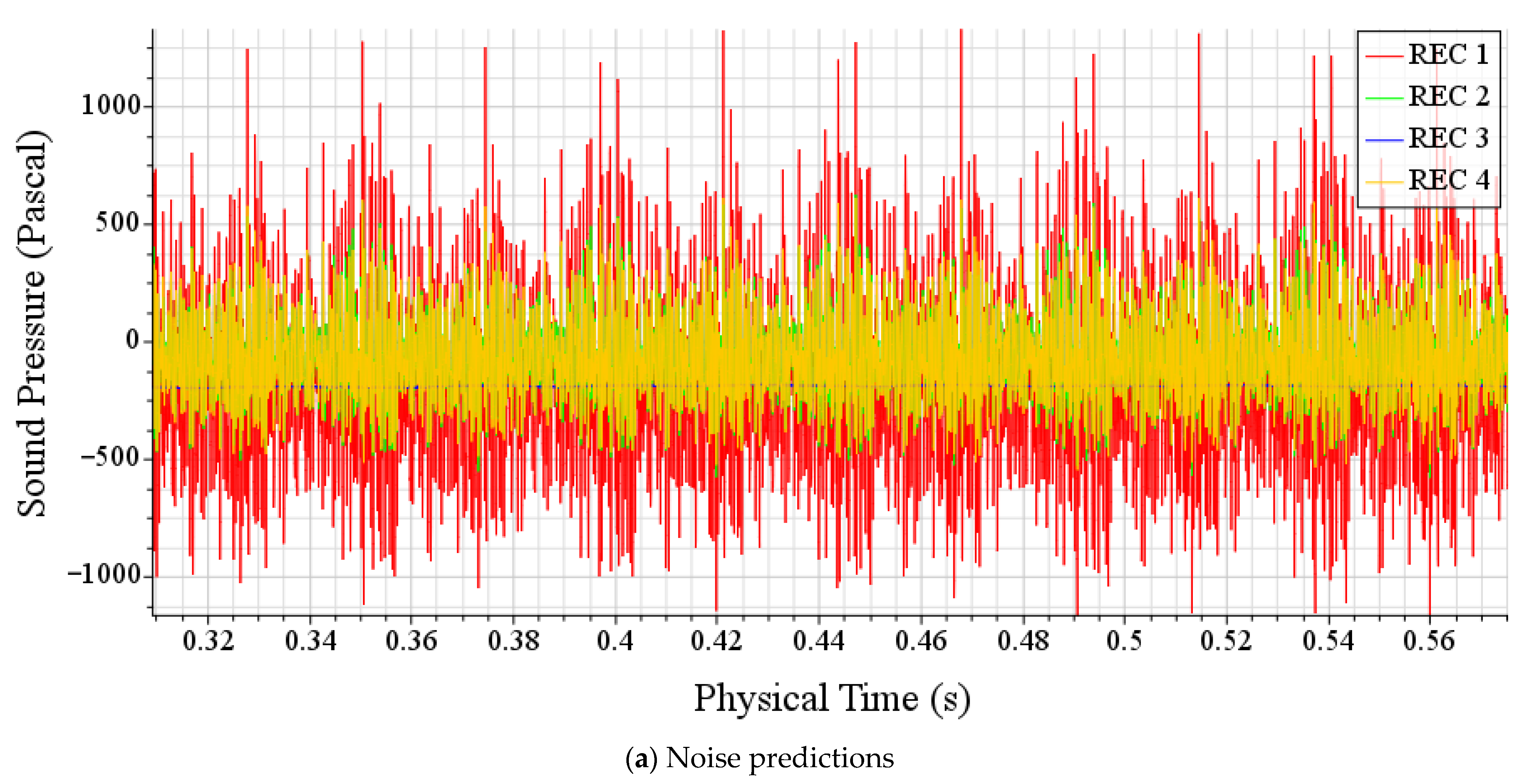
The noise calculations of the four hydrophones in Table 6 are shown in Figure 10a. After reaching a steady state, the detected sound-pressure pulse in 0.3–0.65 s is the same magnitude, showing a periodic change over time. Then, the data are processed via FFT (reference sound pressure is 10⁻⁶ pa), and the frequency distribution of sound-pressure level is obtained, as shown in Figure 10b.

As the propeller periodically rotates and when two detection points have the same radial distance from the origin on the YOZ plane, the side hydrophone, REC2, and the upper REC4 are consistent but slightly different owing to the influence of the propeller rotation. Using the process in Section 2.3, the total noise of each hydrophone position is calculated according to the sound-pressure level, as shown in

Table 7. Total noise pressure at hydrophones.

Hydrophones	REC1	REC2	REC3	REC4
Total sound-pressure level (dB)	143.97	149.58	141.32	149.49

. The results show that the noise of the hydrophone above and on the side of the propeller is larger and similar. The total sound-pressure level of the position of upstream and downstream hydrophones is lower. This shows that the radial noise of the E1619 propeller is higher than the axial noise in this section.

In Figure 10b, in the low-frequency band below 1000 Hz, peaks are evident at 74, 148, 222, 298, 451 and 667 Hz, but not at the upstream REC1 and downstream REC3. In the high-frequency band, the changing trend and peak position of the four measuring points are similar. In open-water, the basic frequency is the blade-passing frequency (BPF), which is 75 Hz (the product of rotation speed and blade number, 10.71 × 7 = 74.94). The frequency positions of several peaks in the low-frequency band are 74, 148, 222, 298 and 451 Hz: the positions of multiple BPFs.

To more intuitively analyze the change in sound-pressure level against frequency, the third octave band is calculated using the formula in Section 2.3 from the continuous fluctuation data of sound-pressure level of each hydrophone, as shown in Figure 11. Referring to Figure 11, the energy of the propeller noise is mainly concentrated in the high-frequency band above 1000 Hz, reaching a peak value in the frequency band of 2500–3000 Hz, which is similar to that found by Özden [28]. In the low-frequency band below 1000 Hz, the sound-pressure level and the distribution of hydrophones at different positions are quite diverse. The difference of trends in sound-pressure level in the high-frequency band is very small.

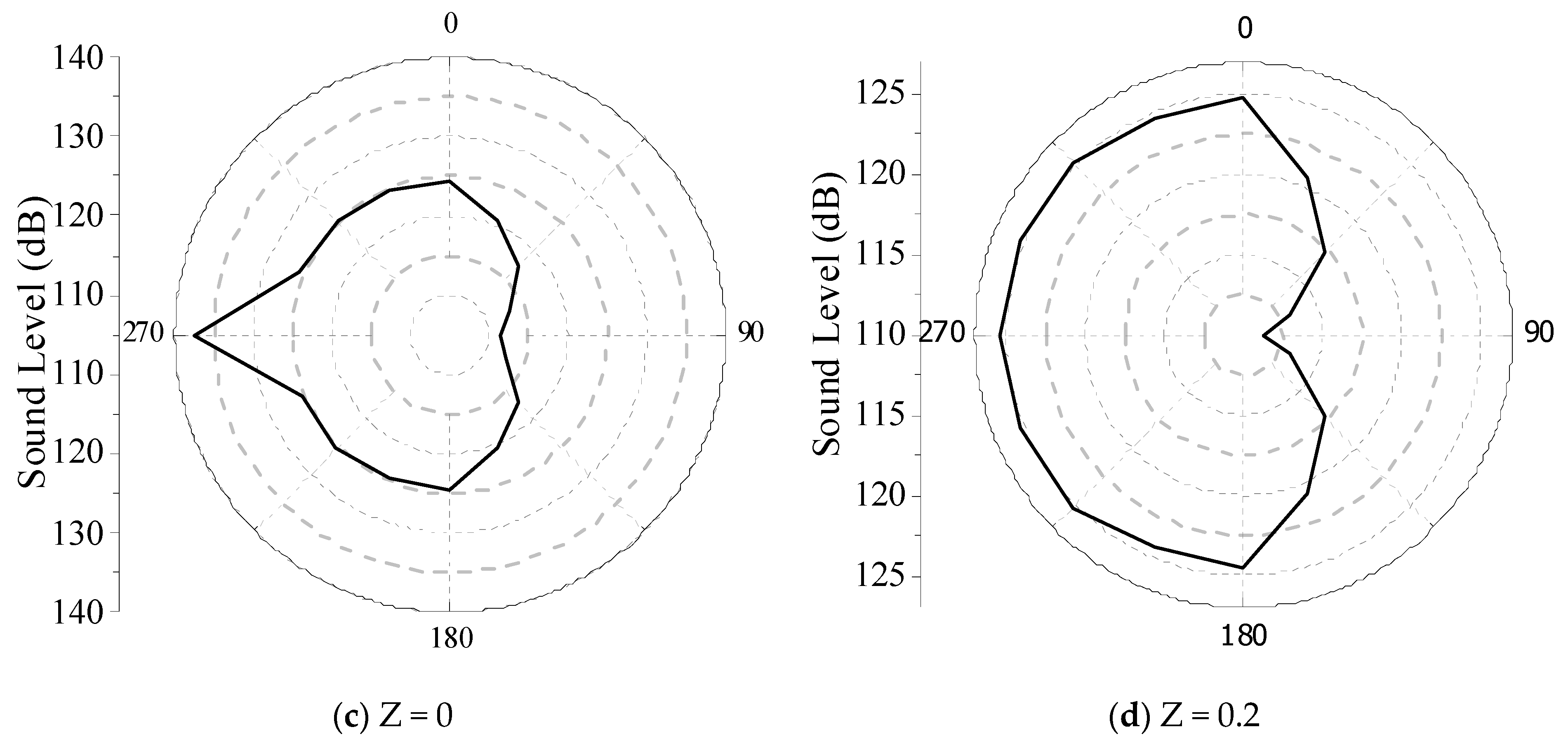
To investigate the propagation characteristics of propeller radiated noise, several hydrophones are evenly distributed at different sections with the projection of the center of the local coordinate system at the center. Sixteen hydrophones are used for each section. After calculating the total sound pressure, a directivity map is drawn, as shown in Figure 12.

Figure 12a,b shows that, in the plane parallel to the propeller disc, the noise propagation pattern of the propeller is basically the same along the circumferential direction. A circle indicates that the radial propagation amplitude of the noise is almost the same. There is a certain degree of attenuation when the noise propagates along the downstream axis, which is consistent with the theoretical prediction. Figure 12c,d shows that the radiation noise in the upstream and downstream of the propeller is relatively low. Compared with the two figures, the noise attenuation along the radial propagation can also be observed. However, compared with Figure 12a,b, the attenuation degree of noise in the radial propagation of equal distance is less than that of the downstream direction.

As shown in Figure 12c, when the uniform flow field J is 0.74, the thickness noise of the E1619 propeller accounts for the main part, and the load noise is smaller than the thickness noise. According to Chang et al. [29], the directional distribution of noise presents a monopole directivity because the thickness noise is generated by the periodic extrusion or expansion of the fluid caused by propeller rotation. The purpose is not to regard the entire propeller as a monopole sound source, but it is instead to distribute the monopole sound sources to the surface of the propeller blade. Therefore, the directivity of the entire propeller on the circumference perpendicular to the propeller disc is not a uniform circle. It is largest in the direction of the propeller disc and smallest in the direction of the shaft. This is because the monopole sound sources arranged on the propeller blade are distributed along the chord length directly onto the propeller. The axial pressures cancel so that the thickness noise in the axial direction of the propeller is the smallest. Thus, the noise directivity graph has an “8” shape. However, owing to the influence of the shaft, the propeller is not symmetrical front to back, which interferes with this acoustic phenomenon. Therefore, the directional chart does not completely resemble an “8” shape.

4.2. Verification of Noise Calculation

The noise of a five-blade propeller model with a diameter of 0.24 m is simulated, and the results are compared with the experimental results and for verification. The propeller model is shown in Figure 13 and the grid for calculation is shown in Figure 14. The grids in the rotating area around the propeller and the wake flow area of the propeller are locally refined. The number of grids is about fourteen million, and the wall y+ is less than one. The propeller speed coefficient is 0.5, rotation speed is 15 rps, and inflow velocity is 1.65 m/s.

The same simulation method of flow field mentioned in the previous section, which is based on the RANS equation and SST k–ω turbulence model, is used. After the hydrodynamic calculation is completed, the FW-H equation is solved to determine the noise.

The position of the hydrophone in the test is 0.6 m away from the center of the propeller in the radial direction. The frequency response range of the hydrophone is 0.1–120,000 Hz. The actual measurement range in the test is 0.1–80,000 Hz. Since the time step is set to 0.00025 s, the upper limit of the corresponding effective frequency is 2000 Hz, and the reference sound pressure is 1 × 10⁻⁶ Pa. Therefore, the test value of 0.1–2000 Hz is selected to compare with the numerical simulation value. The monitoring points are distributed at the same positions as the test hydrophone, and the comparisons between the test values and calculated results are shown in Figure 15 and

Table 8. Comparison of noise calculation results.

	Test Result	Calculation Result
Sound-Pressure Level (dB)	125.88	131

.

It can be seen from Figure 15 that the curve trends obtained by the tests and numerical simulation are similar, and the blade frequency information can be observed clearly in the spectrum curve using numerical calculation. However, the blade frequency information cannot be observed clearly with the increase in frequency. The total sound-pressure level at the hydrophone position is shown in Table 8. The calculation error of noise is within 6 dB. The difference between the total sound-pressure level and the experimental value is not significant, and the reasons for the difference are given below.

(1) The flow-field information collection is different. The thrust torque error between the numerical simulation and test results has a certain influence on the flow field.

(2) The sampling frequency is different; the frequency of numerical simulation is 0—2000 Hz, but the test sampling frequency is 0.1—80,000 Hz.

(3) There is an influence of background noise. Although the experimental values are corrected for the background noise, this influence leads to an error.

Generally, the numerical simulation is in good agreement with the test values, and the few errors are within the acceptable range.

4.3. Submarine Noise during Self-Propulsion

As in Section 4.1, noise-feature prediction is carried out based on self-propulsion simulation with an inflow velocity of 3.051 m/s and a propeller rotation speed of 10.20 rps. The area, including the propeller body and the hull, is the noise source, and several hydrophones are defined. The calculation mesh and model follow the same settings as that of self-propulsion, whereas the physical model uses the previous RANS unsteady calculation. The time step is the time it takes for the propeller to rotate 0.1°.

Table 9. Partial hydrophone positions of submarine self-propulsion noise calculation.

Hydrophone Name	REC1	REC2	REC3	REC4
Position coordinates	(−1, 0, 0)	(0, 1, 0)	(1, 0, 0)	(0, 0, 1)
Location description	1-m upstream	1-m side	1-m downstream	1-m above

shows the position distribution coordinates of the hydrophone using the local coordinate system with the center of the propeller disc as the origin. The description of the coordinate position is based on the local coordinate system.

The post-FFT calculations of the sound-pressure level are shown in Figure 16. There are twelve hydrophones set here. With the center of the propeller disc as the origin, the distances of the near-field, middle-field, and far-field hydrophones are 0.1, 1 and 10 m, respectively. Each distance has four hydrophones, and the distribution is similar to the propeller noise calculation. The noise predictions of different hydrophones are shown in Figure 16. For the case of a pure propeller, REC2 and REC4 distributions are almost the same. However, owing to the wake of the AFF8 hull, the flow field is asymmetric, and the REC2 and REC4 hydrophones show relatively noticeable diversity in the low-frequency band. The diversity of hydrophones at the same distances at different positions is mainly reflected in the low-frequency band below 500 Hz. Generally, the corresponding noise components of each assessment point decrease with the increase in the hydrophone distance, which is consistent with theoretical predictions.

As shown in Figure 16a, in the low-frequency band below 500 Hz, there are many peaks having multiple relationships with the frequency at 40.8 Hz in the spectrum of the side hydrophone near REC2 and that of the upper hydrophone near REC4. However, the spectra of the upstream near REC1 and downstream near REC3 hydrophones have many peaks that are multiples of 71.2 Hz. Observing the phenomenon of peak distribution in Figure 16b,c, with the increase in the distance between hydrophones, the peak distribution of the spectrum becomes more complex. The spectrum of hydrophones at different positions at the same distance has simultaneous multiple peaks of 40.8 and 71.2 Hz. The larger the distance, the more obvious the mix. This is mainly influenced by the hull. When the hydrophone is far away from the origin, the main influence on the sound-pressure is from the propeller to the larger hull. It can be seen from Figure 16 that the peak values of the multiple of axis frequency and multiple of leaf frequency in the low-frequency band show strong line spectrum characteristics, while the spectrum in the high-frequency band shows obvious broadband spectrum characteristics. Simultaneously, the position of the measuring point also has an impact on the spectrum characteristics. The figure shows that the closer the measuring point to the noise source, the wider the low-frequency band with line spectrum characteristics, and that the line spectrum characteristics in the low-frequency band are more obvious.

Similar to the analysis of Section 4.1 and according to the formula in Section 2.3, the one-third-octave band-level spectrum and the total sound pressure of the hydrophone position are calculated, as shown in

Table 10. Total noise pressure at some hydrophones under self-propulsion.

Hydrophones	REC1	REC2	REC3	REC4
Total sound-pressure level (dB)	137.51	124.57	111.24	124.46

and Figure 17. Figure 17 shows diverse distributions of multiple sound pressures at 1000 Hz at four measuring points. The distributions of sound pressure in the high-frequency band above 1000 Hz are similar. This is similar to the open-water condition. However, unlike the open-water propeller, the peak value of the noise-pressure level is in the high-frequency band, which is not evident. After reaching the peak value, the sound-pressure level at the high-frequency band changes little according to frequency. From Figure 17, it can be seen that the noise energy is mainly concentrated in the high-frequency band. Under the same distance, the energy distribution of noise signal is similar at different positions.

Moreover, according to total sound-pressure level in Table 10, those in the upstream are significantly larger, which can be attributed to the influence of the upstream hull.

To investigate the propagation characteristics of the radiated noise when the submarine is sailing, the projection of the central position of the local coordinate system is regarded as the center of the circle, and multiple hydrophones are evenly distributed at different sections so that each section has sixteen hydrophones. After calculating the total sound pressure, the directivity map of sound pressure is drawn, as shown in Figure 18.

Figure 18 shows the law of noise propagation and attenuation under the self-propulsion condition. Figure 18a,b shows the directivity curve of the plane parallel to the propeller disc. In these figures, unlike the propeller, the noise pattern of the submarine under self-propulsion is no longer consistent along the circumferential direction, which is more angular than that of the pure propeller. This is mainly influenced by the appendages. The axial attenuation of noise can be seen by comparing the noise of the two images. Figure 18c,d shows the directivity curve of the plane perpendicular to the propeller disc. Referring to Figure 18c,d, the sound direction is quite different from that of the pure propeller. The noise level of the hydrophone at the downstream position of the propeller still conforms to the situation for which the thickness noise accounts for the main part when the pure E1619 propeller is used, as in Section 4.1. However, the noise level at the upstream of the propeller increases significantly, which can be attributed to the submarine hull being directly connected to the upstream propeller. Compared with Figure 18c,d, even if the hydrophone position is separated from the hull, the radiation noise propagation remains affected by the hull, and the upstream noise is amplified. The radiation noise decays along the propeller radial and axial direction. Furthermore, the upstream noise radial decaying speed is faster.

Figure 19 and Figure 20 show the sound-pressure distribution at different cross sections. At different frequencies, the overall distribution of sound pressure changes, and the difference between high and low frequencies is obvious. In Figure 19, the main contribution of low-frequency noise is the monopole, and there is no clear direction for its development. However, it reflects the characteristics of the quadrupole of the four high-pressure areas distributed at the noise source (propeller) area. When the frequency is greater than 500 Hz, the noise contribution of the quadrupole becomes more evident, and the development trend of the sound field becomes that of the quadrupole extending outwards. The quadrupole term gradually becomes the main contribution to total noise. Figure 20 shows that from the longitudinal section, there are two high-pressure areas near the propeller, and the noise-pressure field develops outwards with these two poles at the center, reflecting dipole characteristics. When the frequency is very high (over 8000 Hz), the development trend of the sound field is also gradually transferred to the quadrupole. Referring to Lighthill [5] and FW–H final form, the total noise can be divided into expressions of monopole, dipole and quadrupole terms. Regarding the flow on the rotating wall, the speed of rotation is small relative to the speed of sound propagation in water, and the monopole and dipole terms are usually the main contributions to noise. Thus, the influence of quadrupole is usually ignored. However, the two figures show that for cases of high frequency, the quadrupole term in the FW–H equation is no longer negligible.

5. Conclusions

Using the CFD method and the FW–H acoustic model, the authors studied the hydrodynamic and noise characteristics of a submarine propeller under self-propulsion. First, the validity of the hydrodynamic calculation of the hull and the propeller was verified. Then, self-propulsion simulation was carried out and the reliability of the calculation was verified using data from the literature. Finally, the analysis and verification of the previous CFD study, the simulation analysis of the propeller’s open-water performance and its noise performance under self-propulsion conditions was carried out. The frequency spectrum of the calculations were then analyzed, and the noise characteristics and rules were discussed. The conclusions are as follows:

• In the noise simulation, the frequency spectrum of the noise source obtained by hydrophones at different positions at the same distance was quite diverse in the low-frequency band below 1000 Hz. However, this was not the case for the high-frequency band above 1000 Hz. Thus, the higher the frequency, smaller is the diversity.
• For the E1619 propeller noise calculation at J = 0.74, the contribution of the thickness surface term was dominant, while that of the load surface term was relatively low.
• The existence of the submarine hull had a significant influence on propeller noise propagation and the upstream noise was amplified.
• When the frequency was low, the monopole and dipole terms of the FW–H equation were usually the main contributors. For cases of high frequency, the quadrupole term was the main contributor and it was no longer insignificant.

The RANS algorithm used in this article has some shortcomings in computational accuracy. The turbulence-resolving ability of RANS is insufficient, particularly when investigating the effects of the quadrupole term in the FW-H equations. Recently, it has been shown that LES having high computational costs may be the best method for reproducing noise sources. Further research may focus on the turbulence model. However, experimental noise data of the E1619 submarine propeller and the DARPA Suboff AFF8 submarine model in open-water conditions are not available publicly. Thus, future research may include the experimental measurement of propeller noise characteristics under different conditions. Optimization of the blade or hull shape might be added in future research based on future numerical simulation and experimental study.

References

1. Roger, M. Fundamentals of aero-acoustics. Lect. Ser.-Van Kareman Inst. Fluid Dyn. 1996, 4, A1–A30. [Google Scholar]
2. Jessup, S.D. An Experimental Investigation of Viscous Aspects of Propeller Blade Flow. Dissertation, School of Engineering and Architecture, Catholic University of America, Washington, DC, USA, 1989. [Google Scholar]
3. Chesnakas, C. Experimental characterization of propeller tip flow. In Proceedings of the 22nd Symposium on Naval Hydrodynamics, Washington, DC, USA, 9–14 August 1998. [Google Scholar]
4. Felli, M.; Grizzi, S.; Falchi, M. A novel approach for the isolation of the sound and pseudo-sound contributions from near-field pressure fluctuation measurements: Analysis of the hydroacoustic and hydrodynamic perturbation in a propeller-rudder system. Exp. Fluids 2014, 55, 1651. [Google Scholar] [CrossRef] [Green Version]
5. Lighthill, M. On Sound Generated Aerodynamically. I. General Theory. Proc. R. Soc. Lond. Ser. A Math. Phys. Sci. 1952, 211, 564–587. [Google Scholar]
6. Curle, N. The Influence of Solid Boundaries upon Aerodynamic Sound. Proc. R. Soc. Lond. Ser. A Math. Phys. Sci. 1955, 231, 505–514. [Google Scholar]
7. Williams, J.E.F.; Hawkings, D.L. Sound generation by turbulence and surfaces in arbitrary motion. Philos. Trans. R. Soc. 1969, A264, 321–342. [Google Scholar]
8. Seol, H.; Suh, J.C.; Lee, S. Prediction of non-cavitating underwater propeller noise. J. Sound Vib. 2002, 257, 131–156. [Google Scholar] [CrossRef] [Green Version]
9. Salvatore, F.; Ianniello, S. Preliminary results on acoustic modelling of cavitating propellers. Comput. Mech. 2003, 32, 291–300. [Google Scholar] [CrossRef]
10. Seol, H.; Suh, J.C.; Lee, S. Development of hybrid method for the prediction of underwater propeller noise. J. Sound Vib. 2005, 288, 345–360. [Google Scholar] [CrossRef]
11. Cianferra, M.; Armenio, V.; Ianniello, S. Hydroacoustic noise from different geometries. Int. J. Heat Fluid Flow. 2018, 70, 348–362. [Google Scholar] [CrossRef] [Green Version]
12. Cianferra, M.; Ianniello, S.; Armenio, V. Assessment of methodologies for the solution of the Ffowcs Williams and Hawkings equation using large-eddy simulations of incompressible single-phase flow around a finite-size square cylinder. J. Sound Vib. 2019, 453, 1–24. [Google Scholar] [CrossRef]
13. Efremov, D.; Milanov, E. Hydrodynamics of DARPA SUBOFF Submarine at Shallowly Immersion Conditions. J. TransNav Int. J. Mar. Navig Saf. Sea Transp. 2019, 13, 337–342. [Google Scholar] [CrossRef] [Green Version]
14. Ling, X.; Leong, Z.; Chin, C.; Woodward, M. Free Surface Effect on the Hydrodynamics of an Underwater Vehicle Hullform. The DARPA SUBOFF. Int. J. Marit. Eng. 2022, 164, A1. [Google Scholar] [CrossRef]
15. Zhu, A.J.; Ying, L.M.; Hu, K.; Shen, H.C. A discussion on the self-propulsion model test method for underwater vessel. J. Ship Mech. 2012, 16, 383–389. [Google Scholar]
16. Brentner, K.S.; Farassat, F. Modeling aerodynamically generated sound of helicopter rotors. Prog. Aerosp. Sci. 2003, 39, 83–120. [Google Scholar] [CrossRef] [Green Version]
17. Qian, X. Ship Propeller Noise; Shanghai Jiaotong University Press: Shanghai, China, 2011. [Google Scholar]
18. Chang, M.S.; Groves, N.C.; Huang, T.T. Geometric Characteristics of DARPA SUBOFF Models DTRC Model Nos. 5470 and 5471; Report No. DTRC/SHD-1298-01; David Taylor Research Center Report: Bethesda, MD, USA, 1998. [Google Scholar]
19. Sezen, S.; Dogrul, A.; Delen, C.; Bal, S. Investigation of self-propulsion of DARPA Suboff by RANS method. Ocean Engin. 2018, 150, 258–271. [Google Scholar] [CrossRef]
20. Liu, H.-L.; Huang, T.-T. Summary of DARPA Suboff Experimental Program Data; Naval Surface Warfare Center, Carderock Division (NSWCCD): West Bethesda, MD, USA, 1998.
21. Crook, B. Resistance for DARPA Suboff as Represented by Model 5470; Report No: DTRC/SHD-1298-07; David Taylor Research Center Report: Bethesda, MD, USA, 1990. [Google Scholar]
22. Chase, N. Simulations of the DARPA Suboff Submarine Including Self-Propulsion with the E1619 Propeller; The University of Iowa: Iowa City, IA, USA, 2012. [Google Scholar]
23. Di Felice, F.; Felli, M.; Liefvendahl, M.; Svennberg, U. Numerical and experimental analysis of the wake behavior of a generic submarine propeller. In Proceedings of the First International Symposium on Marine Propulsors, Trondheim, Norway, June 2009. [Google Scholar]
24. ITTC. Report of Performance Committee; International Towing Tank Conference: Hague, The Netherlands, 1978. [Google Scholar]
25. Brentner, K.S.; Farassat, F. Analytical comparison of the acoustic analogy and Kirchhoff formulation for moving surfaces. AIAA J. 1998, 36, 1379–1386. [Google Scholar] [CrossRef] [Green Version]
26. Frota, J.; Lempereur, P.; Roger, M. Computation of the noise of a subsonic propeller at an angle of attack. In Proceedings of the 4th AIAA/CEAS Aeroacoustics Conference, Toulouse, France, 2–4 June 1988; p. 19982282. [Google Scholar]
27. Marinus, B.; Roger, M.; Van den Braembussche, R.; Bosschaerts, W. Truncated method for propeller noise prediction up to low supersonic helical tip Mach numbers. In Proceedings of the 15th AIAA/CEAS Aeroacoustics Conference, Miami, FL, USA, 11–13 May 2009; p. 3330. [Google Scholar]
28. Özden, M.C.; Gürkan, A.Y.; Özden, Y.A.; Canyurt, T.G.; Korkut, E. Underwater radiated noise prediction for a submarine propeller in different flow conditions. Ocean Eng. 2016, 126, 488–500. [Google Scholar] [CrossRef]
29. Chang, X.; Xin, K.; Ye, L.; Wang, C. Prediction on non-cavitating noise performance of contra-rotating propeller and influencing factors analysis. J. Harbin Engin Univ. 2018, 39, 635–643. [Google Scholar]
Figure 1. E1619 propeller.
Jmse 11 01206 g001
Figure 2. DARPA SuboffAFF8 model with propeller.
Jmse 11 01206 g002
Figure 3. Mesh generation of DARPA Suboff AFF8 model.
Jmse 11 01206 g003
Figure 4. Pressure distribution of DARPA Suboff AFF8.
Jmse 11 01206 g004
Figure 5. Contours of axial velocity distribution of submarines at different cross sections (dimensionless velocity component is x-axis direction).
Jmse 11 01206 g005
Figure 6. Calculation area division and grid densification of propeller open-water calculation.
Jmse 11 01206 g006
Figure 7. Comparison of open-water and experimental values.
Jmse 11 01206 g007
Figure 8. Division of area of submarine self-propulsion calculation.
Jmse 11 01206 g008
Figure 9. Single blade thrust, torque and pulsation under self-propulsion.
Jmse 11 01206 g009
Figure 10. Comparison of open-water noise prediction of different hydrophones at J = 0.74.
Jmse 11 01206 g010aJmse 11 01206 g010b
Figure 11. One-third frequency-band level of each hydrophone in open-water.
Jmse 11 01206 g011
Figure 12. Directivity of sound pressure at different sections (0° points to positive direction of y axis) in open-water.
Jmse 11 01206 g012
Figure 13. Propeller model for noise test.
Jmse 11 01206 g013
Figure 14. Mesh generation of the test propeller.
Jmse 11 01206 g014
Figure 15. Comparison of noise calculation results.
Jmse 11 01206 g015
Figure 16. Sound-pressure levels under self-propulsion. (a) Sound-pressure levels of near-field hydrophones, (b) Sound-pressure levels of middle-distance hydrophones, (c) Sound-pressure levels of far-field hydrophones.
Jmse 11 01206 g016
Figure 17. One-third frequency-band level of medium distance hydrophones under self-propulsion.
Jmse 11 01206 g017aJmse 11 01206 g017b
Figure 18. Directivity of sound pressure at different sections (0° points to positive direction of y axis) under self-propulsion.
Jmse 11 01206 g018aJmse 11 01206 g018b
Figure 19. Distribution of sound pressure at different frequencies at X = 0.2.
Jmse 11 01206 g019
Figure 20. Distribution of sound pressure at different frequencies at Z = 0.2.
Jmse 11 01206 g020